Uniform Test on the Mixture Simplex Region

Abstract

For the symmetrical mixture model and mixture test area, the lattice point set is used to partition, and then the corresponding test statistics can be constructed. In this paper, we first propose the partition methods under the lattice point sets and obtain several sub-simplexes without common interior points. Furthermore, we present a method for constructing a uniform design on the simplex using the center points of these sub-simplexes. The designs satisfy the uniformity of maximum distance deviation and provide good results for the mean square error deviation. Finally, the uniformity test on the mixture region is considered and illustrated by examples.

1. Introduction

For production and scientific experiments, it is necessary to constantly improve the quality of products and develop new products. However, it is a challenge to arrange the experiments effectively and analyze scientifically the results. Experimental designs provide various practical methods for solving these challenges, closely related to production and scientific research, enriching and developing theoretically and methodologically. Mixture experimental design is an essential part of experimental design and is widely used in many fields.

Since Scheff (1958) [1] first introduced the notion and theory of mixture experimental designs, it has developed substantially and led to numerous theoretical results in this field with the development of experimental design theory. However, there are two main designs in this direction. The first is the optimal design for the mixture experiments based on various optimality criteria. The second is uniform designs for mixture experiments concerning uniformity and robustness. The optimal design for mixture experiments is to study the optimization problems on irregular mixture experimental regions based on the optimal design theory.

The theory of optimal design aims to present a criterion for statistically evaluating the quality of designs and constructing optimal designs by these criteria. Kiefer [2,3] organized the previous results and extended the concept of discrete experimental designs to continuous designs. Furthermore, Kiefer [2,3] presented various optimal design criteria (e.g., $D-$optimal, $A-$optimal, and $I_{\lambda }-$optimal) and also proved the optimal design equivalence theorem, which is the foundation for establishing and developing optimal design theory. Moreover, many statisticians have proposed different optimal design criteria based on the factual background.

However, as Fang and Wang (1994) [4] pointed out, the optimal design has drawbacks such as a lack of robustness and many points distributed at the boundary. To improve the design, Fang and Wang (1994) [4] constructed a uniform design by using the number-theoretic methods. Further, Wang and Fang (1996) [5] presented uniform designs for mixture experiments by extending the idea of uniform design to mixture experiments. These designs consider evenly distributed n experimental points on the mixture domain and do not allow replication. There are two commonly used methods for obtaining uniformly distributed design points on the mixture region, which are the inverse permutation method proposed by Wang and Fang (1990) [6] and the numerical optimization method. Moreover, numerous pieces of literature have extended these methods; see [7,8]. Li and Zhang (2017) [9] proposed a pseudo-component transform design based on the Scheffé-type design, which combines optimality and uniformity, and discussed the uniformity of the lattice point sets. Kim and Kim (2020) [10] proved that the conjecture proposed by Li and Zhang (2017) [9] on a property of the proposed component transform is not true in the general case, and further refined the conjecture and gave a proof of the result.

Lattice design is an essential method for mixture experimental design, which mainly considers arranging experiments on two classes of lattice point sets of the simplex region, i.e., central lattice point sets and q-component m-order lattice point sets. The goal of the simplex lattice design is to reasonably assign the weights of each component to distribute each weight of the mixture components evenly in the design space and then test each weight separately based on its distribution to find the best formula for production. It has been widely used in agriculture, biology, medicine, engineering, etc.; see [11,12,13,14,15], among other related literature. Moreover, it is also mentioned in Li et al. (2021) [16] that lattice point sets can be used for non-parametric modeling and uniformity testing. However, when the test domain is an irregular convex polyhedron, the simplex lattice point design based on Scheff(1958) [1] is not feasible, and it is, therefore, a challenge to efficiently arrange the experimental points on the region. We now propose to partition the irregular convex polyhedra to obtain the experimental points inside the convex polyhedra by applying the theory of lattice point design for mixture experiments. However, there are issues such as how to effectively partition the test region and how to ensure that the number of experimental points is as small as possible and the amount of information obtained from the experiment is maximized. For this purpose, we consider the problem of the uniformity test of experimental points in the symmetric experimental region, make the experimental points distributed as uniformly as possible in the experimental region, and construct the uniformity test on the symmetric experimental region with the following three advantages: (1) the uniformity test statistic of the test point distribution on a simple shaped experimental region can be constructed; (2) the resulting test statistic can be used to measure the degree of uniformity of a design; (3) under this method, a uniform partitioning of a symmetric experimental domain can be obtained.

Li et al. (2020) [17] proposed a graph checking method to verify the optimality of the symmetrical design of a mixture. The effectiveness of this method can be shown by case analysis. Lattice point sets are essential tools for mixture experiments, which provide an optimal design for a given model, uniformly distribute on the simplex region, and have good space-filling properties; see He [18,19]. Therefore, in this paper, we first consider the method of partitioning for the symmetrical mixture region to obtain several sub-simplexes without common interior points and construct a uniform design for the mixture experiments under this partitioning method. Further, the uniformity of the design points on the mixture experimental region is tested, the method’s effectiveness is verified with examples, and further research questions are suggested.

The rest of the paper is organized as follows. Elementary concepts of mixture experiment and uniform design, notation, and definitions are given in Section 2. In Section 3, the method of the partitioning of mixture experimental regions is given. Section 4 provides a method and steps for constructing a uniform design using a lattice point partition design. The uniformity test statistic on the mixture experimental region is constructed, and the steps for the detailed test are given in Section 5. In Section 6, two examples show that the lattice point partitioning method is feasible and valid for uniformity testing of the design point distribution using the uniformity test statistic.

2. Preliminaries

Mixture experiments (see Cornell (2002) [11]) are experiments in which two or more components are blended in the same or different proportions, and their response of interest is recorded for each blend. For the q-component mixture system, the response is a function of each component $x_1,x_2,\cdots ,x_q$. The mixture region determined by the proportion of each component can be expressed as

$$\mathcal{X}=\left\{{\left(x_1,x_2,\cdots ,x_q\right)}^{\mathrm{T}}:\sum _{i=1}^q{x}_i=1,x_i\ge 0,i=1,2,\cdots ,q,C^{\prime }s\right\},$$

where the $C^{\prime }s$ is an additional constraint condition. In addition, we denote $\mathcal{X}$ as $S^{q-1}$ if the component is without any constraints.

However, there are additional constraints on the mixture components besides the primary constraints for many practical situations. The additional constraint $C^{\prime }s$ commonly exists in mixture experiments as follows.

1. Single-Component Constraints (SCCs)

$$C^{\prime }s:0\le a_j\le x_j\le b_j\le 1,j=1,2,\cdots ,q.$$

2. Multiple-Component Constraints (MCCs)

$$C^{\prime }s:0\le a_j\le \sum _{i=1}^q{c}_{ji}{x}_i\le b_j,j=1,2,\cdots ,m.$$

3. Nonlinear Component Constraints (NCCs)

$$C^{\prime }s:a_j\le {\varphi }_j\left(x_1,x_2,\cdots ,x_q\right)\le b_j,j=1,2,\cdots ,l,$$

where $a_j,b_j$ and $c_{ji}$ are known constants, and ${\varphi }_j\left(x_1,x_2,\cdots ,x_q\right)$ are nonlinear functions for each component.

Let $\mathbf{a}={(a_1,a_2,\cdots ,a_q)}^{\mathrm{T}}$, $\mathbf{b}={(b_1,b_2,\cdots ,b_q)}^{\mathrm{T}}$; for convenience, we denote

$$\begin{array}{c}\hfill S_{\left[\mathbf{a},\mathbf{b}\right]}^{q-1}=\left\{\mathbf{x}=\left(x_1,\cdots ,x_q\right):\mathbf{x}\in S^{q-1},0\le a_i\le x_i\le b_i\le 1,i=1,\cdots ,q\right\}\end{array}$$

(1)

as the mixture experimental regions with upper and lower bound constraints. Then,

$$S^{q-1}=S_{[\mathbf{0},\mathbf{1}]}^{q-1},$$

(2)

where $\mathbf{0}$ and $\mathbf{1}$ are vectors of 0s and 1s, respectively.

Definition 1.

Let $m\le q$ be a positive integer, if there exists ${\alpha }_1,{\alpha }_2,\cdots ,{\alpha }_q\in {\mathbb{Z}}^{+}$, such that ${\alpha }_1+{\alpha }_2+\cdots +{\alpha }_q=m$. Then, the q components m-order lattice point sets can be defined as

$$\begin{array}{c}\hfill \mathcal{L}\{q,m\}=\left\{{(\frac{{\alpha }_1}{m},\frac{{\alpha }_2}{m},\cdots ,\frac{{\alpha }_q}{m})}^{\mathrm{T}}:\sum _{i=1}^q{\alpha }_i=m,{\alpha }_j\in {\mathbb{Z}}^{+},j=1,2,\cdots ,q\right\}.\end{array}$$

(3)

From Definition 1, we obtain that the lattice point set $\mathcal{L}\{q,m\}$ contains $\left(\genfrac{}{}{0pt}{}{q+m-1}{m}\right)$ points which uniformly distribute on the mixture region $S^{q-1}$. To present the construction method for uniform designs under the lattice point sets, we firstly provide three common criteria for measuring the uniformity distribution of design points.

Suppose that ${\mathcal{P}}_n=\left\{{\mathbf{x}}_1,{\mathbf{x}}_2,\cdots ,{\mathbf{x}}_n\right\}\subset \mathcal{X}\subseteq S^{q-1}$ is a set. Then, the distance between a point $\mathbf{x}$ and the point set ${\mathcal{P}}_n$ can be defined as

$$d^2(\mathbf{x},{\mathcal{P}}_n)=\underset{1\le i\le n}{min}\left\{d^2(\mathbf{x},{\mathbf{x}}_i)\right\},$$

(4)

where $d^2(\mathbf{x},{\mathbf{x}}_i)={∥\mathbf{x}-{\mathbf{x}}_i∥}^2$.

Therefore, there are three deviation criteria that are commonly used to measure the uniformity of the point set ${\mathcal{P}}_n$, which can be given as follows.

1. Mean Square Error Deviation (MSED)

$$\mathrm{MSED}\left({\mathcal{P}}_{\mathrm{n}}\right)=\mathrm{E}\left({\mathrm{d}}^2(\mathbf{x},{\mathcal{P}}_{\mathrm{n}})\right)=\frac{1}{\mathrm{Vol}\left(\mathcal{X}\right)}{\int }_{\mathcal{X}}\underset{1\le \mathrm{j}\le \mathrm{n}}{min}\left\{{\mathrm{d}}^2(\mathbf{x},{\mathbf{x}}_{\mathrm{j}})\right\}\mathrm{d}\mathbf{x},$$

where $\mathrm{Vol}\left(\mathcal{X}\right)$ is the volume of $\mathcal{X}$.

2. Root Mean Square Error Deviation (RMSD)

$$\mathrm{RMSD}\left({\mathcal{P}}_{\mathrm{n}}\right)=\sqrt{\mathrm{E}\left({\mathrm{d}}^2(\mathbf{x},{\mathcal{P}}_{\mathrm{n}})\right)}.$$

3. Maximum Distance Deviation (MD)

$$\mathrm{MD}\left({\mathcal{P}}_{\mathrm{n}}\right)=\underset{\mathbf{x}\in \mathcal{X}}{max}\left\{{\mathrm{d}}^2(\mathbf{x},{\mathcal{P}}_{\mathrm{n}})\right\}.$$

However, the calculation of the above three deviations is complicated when there are more components in the mixture experiments, and an approximation is used instead in practice. Let

$$\begin{array}{c}\hfill \begin{array}{c}\mathrm{msed}\left({\mathcal{P}}_{\mathrm{n}}\right)=\frac{1}{\mathrm{N}}{\displaystyle \sum _{{\mathbf{t}}_{\mathrm{k}}\in \mathcal{L}}}{\mathrm{d}}^2({\mathbf{t}}_{\mathrm{k}},{\mathcal{P}}_{\mathrm{n}}),\hfill \\ \mathrm{rmsd}\left({\mathcal{P}}_{\mathrm{n}}\right)=\sqrt{\frac{1}{\mathrm{N}}{\displaystyle \sum _{{\mathbf{t}}_{\mathrm{k}}\in \mathcal{L}}}{\mathrm{d}}^2({\mathbf{t}}_{\mathrm{k}},{\mathcal{P}}_{\mathrm{n}})},\hfill \\ \mathrm{md}\left({\mathcal{P}}_{\mathrm{n}}\right)=\underset{{\mathbf{t}}_{\mathrm{k}}\in \mathcal{L}}{max}\left\{{\mathrm{d}}^2({\mathbf{t}}_{\mathrm{k}},{\mathcal{P}}_{\mathrm{n}})\right\},\hfill \end{array}\end{array}$$

(5)

where $\mathcal{L}=\left\{{\mathbf{t}}_1,{\mathbf{t}}_2,\cdots ,{\mathbf{t}}_N\right\}$ is a NT-net in $\mathcal{X}$, which is composed of the set of random mixture points obeying a uniform distribution.

3. Partition Methods for the Mixture Region

Now, to construct a uniform design for mixture experiments, we first need to partition for the mixture region $\mathcal{X}$. Since the NCC mixture region is not a convex polyhedron, there may be no extreme vertices existing on the boundary. The MCC and SCC mixture region $\mathcal{X}\subset S^{q-1}$ both are convex polyhedra interior to the $S^{q-1}$. Here, we only discuss the partition of MCC and SCC mixture regions and first briefly describe the two partitioning methods presented by Li et al. (2020) [17], and the method of lattice point set partition for the SCC mixture region will also be presented.

First, we give the following notations where $s_i^k$ is the ith $k-$dimensional cell of a convex polyhedron. Then,

(1)

$s_i^0$ represents the ith vertex of a convex polyhedron;

(2)

$s_j^1$ represents the jth edge of a convex polyhedron;

(3)

$s_k^2$ represents the kth surface of a convex polyhedron;

(4)

$s_l^{q-2}$ represents the lth $q-2$ dimensional boundary of a convex polyhedron;

(5)

$s_1^{q-1}=\mathcal{X}$ represents a convex polyhedron of the mixture region.

Based on the above notations, there are two main partition methods of mixture regions as presented by Li et al. (2020) [17].

3.1. Vertex Partitioning Method

Step 1. Let N points $s_1^0,s_2^0,\cdots ,s_N^0$ on the $\mathcal{X}=s_1^{q-1}$, the convex polyhedron  $s_1^{q-1}=\{s_1^0,s_2^0,\cdots ,s_N^0\}.$

Step 2. Starting from the first vertex $s_1^0$, we then obtain all the $q-2$-dimensional cells do not contain the vertex $s_1^0$. That is, $s_i^{q-2}=\left\{s_{i_1}^0,s_{i_2}^0,\cdots ,s_{i_k}^0\right\},i=1,2,\cdots ,l,$ and $i_1<i_2<\cdots <i_k$; the k may be unequal for different i.

Step 3. From each of the $s_i^{q-2}$, find each of the $q-3$-dimensional cell cavities that do not contain $s_{i_1}^0$, and work out the branching step by step until the low-dimensional cell cavities are reached.

Step 4. Suppose that there are g cell sequences satisfying the above steps. Then,

$$s_i^0\subset s_i^1\subset \cdots \subset s_i^{q-2}\subset s_1^{q-1},i=1,2,\cdots ,g.$$

(6)

Take the first vertex of each of the q cells from (6), and these q vertices compose a $q-$ 1 dimensional sub-simplex. Such g sub-simplexes have no common interior points with each other, which is a partition for the given mixture convex polyhedron.

3.2. Central Partition Method

Step 1. Let $s_0^0$ be the center of the mixture convex polyhedron.

Step 2. We obtain several $q-1$-dimensional simplexes without common interior points, which are composed of $s_0^0$ and all vertices of each $q-2$-dimensional edge.

Step 3. Suppose that $s_i^{q-2}$ has $n_i$ vertexes that are connected by a one-dimensional edge of $n_i$; then, find the vertices on both ends of each one-dimensional edge. Renumber the vertices of $n_i$, such that $s_{i_1}^1=\{s_{i_1}^0,s_{i_2}^0\},s_{i_2}^1=\{s_{i_2}^0,s_{i_3}^0\},\cdots ,s_{n_i}^1=\{s_{n_i}^0,s_{i_1}^0\},$ and obtain the $n_i$ one-dimensional edge of $s_i^{q-2}$.

Step 4. Divide $s_i^{q-2}$ into $n_i-q+2$ sub-simplex without a common interior point

$$\{s_{i_1}^0,s_{i_2}^0,\cdots ,s_{i_{q-1}}^0\},\{s_{i_1}^0,s_{i_3}^0,\cdots ,s_{i_q}^0\},\cdots ,\{s_{i_1}^0,s_{n_i-q-2}^0,\cdots ,s_{n_i}^0\}.$$

(7)

The combination of $s_0^0$ and each of (7) constitutes $n_i-q+2$ sub-simplexes with $(q-1)$-dimensions. It is noted that these ${\sum }_{i=1}^l(n_i-q+2)$ sub-simplexes have no common interior points with each other and this is a partition of the given convex polyhedron.

3.3. Partition Method of Lattice Point Sets for the Simplex $S^{q-1}$

Now, we will provide a partition method by using the lattice point sets $\mathcal{L}\{q,m\}$. As shown in Algorithm 1.

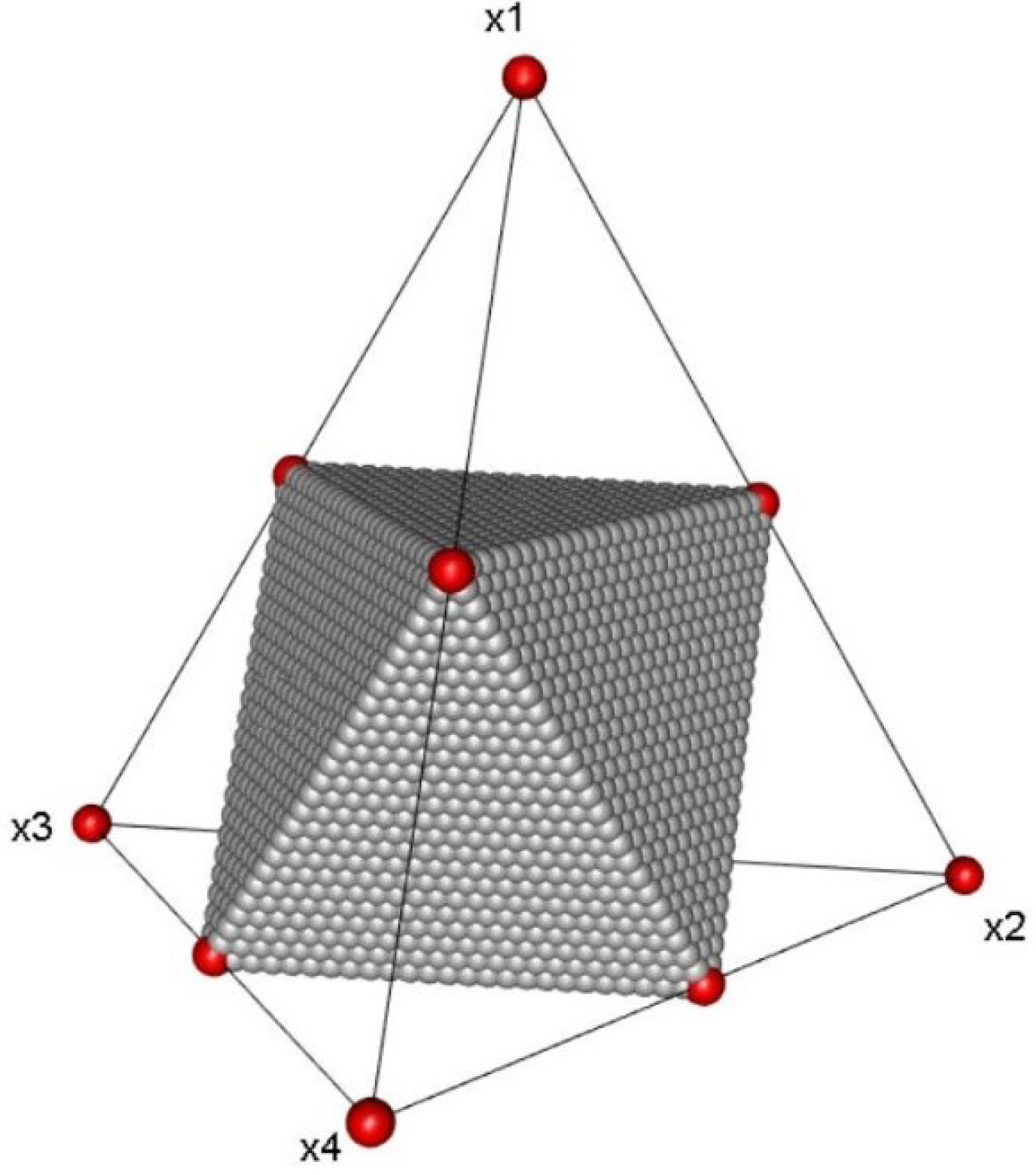
For example, using the above method, the simplex $S^{3-1}$ can be partitioned into 4 sub-simplexes under the $\mathcal{L}\{3,2\}$ and partitioned into 9 sub-simplexes under the $\mathcal{L}\{3,3\}$. In particular, the simplex $S^{3-1}$ can be partitioned into $m^2$ sub-simplexes under the $\mathcal{L}\{q,m\}$, and these sub-simplexes are congruent. Furthermore, for $q=4$, the case of partitioning is more complex, but $S^{4-1}$ also can be partitioned into 8 sub-simplexes under the $\mathcal{L}\{4,2\}$ and we can find that the sub-region $S_{[0,0.5]}^{4-1}$ contains 4 sub-simplexes and 6 extreme vertices, as shown in Figure 1. In addition, for $q=5$, $S^{5-1}$ also can be partitioned into 16 sub-simplexes under the $\mathcal{L}\{5,2\}$ and the sub-region $S_{[0,0.5]}^{5-1}$ contains 11 sub-simplexes, but we find that the volumes of these 11 sub-simplexes and the other 5 sub-simplexes are not congruent. It is more complex when the order of the lattice point set is higher.

Algorithm 1: Partition for simplex $S^{q-1}$

Step 1. Let $S_{[\mathbf{a},\mathbf{b}]}^{q-1}=\{\mathbf{x}={(x_1,x_2,\cdots ,x_q)}^{\mathrm{T}}:0\le a_i\le x_i\le b_i\le 1,i=1,2,\cdots ,q,\mathbf{x}\in S^{q-1}\}$ be a mixture region with upper constraints ${\mathbf{b}}^{\mathrm{T}}=(b_1,b_2,\cdots ,b_q)$ and lower constraints ${\mathbf{a}}^{\mathrm{T}}=(a_1,a_2,\cdots ,a_q)$. Step 2. Suppose that $0,\frac{1}{m},\cdots ,\frac{m-1}{m}$ are the m levels of the q-factor and let ${\mathbf{l}}_m={(0,\frac{1}{m},\cdots ,\frac{m-1}{m})}^{\mathrm{T}}$. Construct two fully factorial design matrices with q-factor m levels $$\overline{\mathbf{L}}=\left({\mathbf{l}}_m\otimes {\mathbf{1}}_{m^{q-1}},{\mathbf{1}}_m\otimes {\mathbf{l}}_m\otimes {\mathbf{1}}_{m^{q-2}},{\mathbf{1}}_{m^2}\otimes {\mathbf{l}}_m\otimes {\mathbf{1}}_{m^{q-3}},\cdots ,{\mathbf{1}}_{m^{q-1}}\otimes {\mathbf{l}}_m\right),$$ $\overline{\mathbf{U}}=\frac{1}{m}{\mathbf{J}}_{N_0\times q}+\overline{\mathbf{L}}$, where $N_0=m^q$, ${\mathbf{1}}_m$ is a m-dimensional vector with all elements of 1, and ${\mathbf{J}}_{N_0\times q}$ is a $N_0\times q$ matrix with all elements of 1. Step 3. Let $\overline{\mathbf{L}}{\mathbf{1}}_q={\left({\overline{\mathbf{l}}}_1,{\overline{\mathbf{l}}}_2,\cdots ,{\overline{\mathbf{l}}}_{N_0}\right)}^{\mathrm{T}},\overline{\mathbf{U}}{\mathbf{1}}_q={\left({\overline{\mathbf{u}}}_1,{\overline{\mathbf{u}}}_2,\cdots ,{\overline{\mathbf{u}}}_{N_0}\right)}^{\mathrm{T}}$, where ${\overline{\mathbf{l}}}_i$ is the ith element in $\overline{\mathbf{L}}{\mathbf{1}}_q$, and ${\overline{\mathbf{u}}}_j$ is the jth element in $\overline{\mathbf{U}}{\mathbf{1}}_q$, $i,j=1,2,\cdots ,N_0$. If $I({\overline{\mathbf{l}}}_{i_j}<1)I({\overline{\mathbf{u}}}_{i_j}>1)=1,j=1,2,\cdots ,r$ and let ${\mathbf{E}}_r={\left({\mathbf{e}}_{N_0}\left(i_1\right),{\mathbf{e}}_{N_0}\left(i_2\right),\cdots ,{\mathbf{e}}_{N_0}\left(i_r\right)\right)}^{\mathrm{T}}$. Then, the upper and lower bound matrices within the simplex are $\mathbf{L}={\mathbf{E}}_r\overline{\mathbf{L}}={\left({\mathbf{a}}_1,{\mathbf{a}}_2,\cdots ,{\mathbf{a}}_r\right)}^{\mathrm{T}}$ and $\mathbf{U}={\mathbf{E}}_r\overline{\mathbf{U}}={\left({\mathbf{b}}_1,{\mathbf{b}}_2,\cdots ,{\mathbf{b}}_r\right)}^{\mathbf{T}}$, respectively. Step 4. Obtain a partition for the simplex $S^{q-1}$. That is, $$S^{q-1}=\underset{j=1}{\overset{r}{\cup }}{S}_{[{\mathbf{a}}_j,{\mathbf{b}}_j]}^{q-1},$$ (8) where $\mathbf{a}=\left(a_{j1},a_{j2},\cdots ,a_{jq}\right)$ and $\mathbf{b}=\left(b_{j1},b_{j2},\cdots ,b_{jq}\right)$ are the elements of the j row of the matrix $\mathbf{L}$ and $\mathbf{U}$, respectively.

Moreover, if the $S_{[{\mathbf{a}}_j,{\mathbf{b}}_j]}^{q-1},j=1,2,\cdots ,r$ is a mixture simplex, then it can be further partitioned using the method above.

Theorem 1.

Suppose that ${\mathbf{x}}_1,{\mathbf{x}}_2,\cdots ,{\mathbf{x}}_q\in S^{q-1}$ are q linearly independent design points, $V^q=V\{{\mathbf{x}}_1,{\mathbf{x}}_2,\cdots ,{\mathbf{x}}_q\}\subset S^{q-1}$ is a $q-1$ dimensional sub-simplex composed of these q design points and $\mathbf{X}={\left[{\mathbf{x}}_1,{\mathbf{x}}_2,\cdots ,{\mathbf{x}}_q\right]}^{\mathrm{T}}$ is a matrix consisting of these vertices arranged in rows. Let

$$\begin{array}{c}\hfill \mathbf{H}=\left(\begin{array}{ccccccc}(q-1)h_1& 0& 0& \cdots & 0& 0& h_q\\ -h_1& (q-2)h_2& 0& \cdots & 0& 0& h_q\\ -h_1& -h_2& (q-3)h_3& \cdots & 0& 0& h_q\\ -h_1& -h_2& -h_3& \cdots & 0& 0& h_q\\ ⋮& ⋮& ⋮& \ddots & ⋮& ⋮& ⋮\\ -h_1& -h_2& -h_3& \cdots & 2h_{q-2}& 0& h_q\\ -h_1& -h_2& -h_3& \cdots & -h_{q-2}& h_{q-1}& h_q\\ -h_1& -h_2& -h_3& \cdots & -h_{q-2}& -h_{q-1}& h_q\end{array}\right),\end{array}$$

(9)

where $h_i=1/\sqrt{(q-i)(q-i+1)},i=1,2,\cdots ,q-1,h_q=1/\sqrt{q}.$ Denote $\mathbf{W}=\mathbf{X}\mathbf{H}{\left[{\mathbf{I}}_{q-1},\mathbf{0}\right]}^{\mathrm{T}}={\left\{{\omega }_{ij}\right\}}_{i,j=1}^{q,q-1}$ and $\overline{\mathbf{W}}={\{{\omega }_{ij}-{\omega }_{1j}\}}_{i=2,j=1}^{q,q-1}$. Then, the volume of the sub-simplex V is

$$\mathrm{Vol}\left(V^q\right)=\frac{1}{(q-1)!}det\left(\overline{\mathbf{W}}\right).$$

Proof of Theorem 1. 

Let

$${\mathbf{W}}^{{}^{\prime }}=(q-1)(q\mathbf{X}-{\mathbf{J}}_q)\mathbf{H}\left(\begin{array}{c}{\mathbf{I}}_{q-1}\\ \mathbf{0}\end{array}\right)={\left\{w_{ij}^{{}^{\prime }}\right\}}_{i,j=1}^{q,q-1},$$

and we first map the simplex V to ${\mathcal{I}}^{q-1}$ by using the independent transformation method of simplex vertices. Denote ${\omega }_i^{{}^{\prime }}={({\omega }_{i1}^{{}^{\prime }},{\omega }_{i2}^{{}^{\prime }},\cdots ,{\omega }_{i2}^{{}^{\prime }})}^{\mathrm{T}},i=1,2,\cdots ,q$ are q points in ${\mathcal{I}}^{q-1}$. For any two points ${\mathbf{x}}_{\mathbf{i}},{\mathbf{x}}_{\mathbf{j}}\in {\mathbf{S}}^{\mathbf{q}-\mathbf{1}}$, there exist two image points ${\omega }_i,{\omega }_j\in {\mathcal{I}}^{q-1}$ corresponding to ${\mathbf{x}}_{\mathbf{i}}$ and ${\mathbf{x}}_{\mathbf{j}}$, respectively. Then,

$$d_S=d({\mathbf{x}}_i,{\mathbf{x}}_j)=\frac{1}{q(q-1)}d({\omega }_i,{\omega }_j)=d_{\mathbf{w}}.$$

Let $\lambda =\frac{d_s}{d_w}=\frac{q}{q-1}$, and we have

$$\mathbf{W}=\lambda {\mathbf{W}}^{{}^{\prime }}=q(q-1){\mathbf{W}}^{{}^{\prime }}={\left\{{\omega }_{ij}\right\}}_{i,j=1}^{q,q-1}.$$

Further, we obtain that the convex polyhedron W is composed of these points ${\omega }_i={({\omega }_{i1},{\omega }_{i2},\cdots ,{\omega }_{i2})}^{\mathrm{T}},i=1,2,\cdots ,q$ in ${\mathcal{I}}^{q-1}$ and the sub-simplex $V\in S^{q-1}$, which are congruent. Then,

$$\mathrm{Vol}\left(V\right)=\mathrm{Vol}\left(W\right)=\frac{1}{(q-1)!}\left|\det \left([0,{\mathbf{I}}_{q-1}]\mathbf{W}-{\mathbf{1}}_{q-1}\left({\mathbf{e}}_1^{\mathrm{T}}\mathbf{W}\right)\right)\right|=\frac{1}{(q-1)!}det\left(\overline{\mathbf{W}}\right).$$

□

We note that each sub-simplex in the partitioned simplex is composed of q adjacent lattice points, and if $\mathbf{x}\in \mathcal{L}\{q,m\}\subset S^{q-1}$, then the lattice points that are adjacent to $\mathbf{x}$ can be defined as

$${\mathbf{x}}^{\prime }=\mathbf{x}+\frac{1}{m}{\mathbf{e}}_q\left(i\right)-\frac{1}{m}{\mathbf{e}}_q\left(j\right),i,j=1,2,\cdots ,q,$$

where ${\mathbf{e}}_q\left(i\right)$ is a q-dimensional column vector with the ith element being 1 and all other elements 0, and $i\ne j,{\mathbf{x}}^{\prime }\in \mathcal{L}\{q,m\}$.

Therefore, it is found that in the simplex $S^{q-1}$, the matrix ${\mathbf{V}}_1$ consisting of the vertices of the sub-simplex $V_1$ with $(1,0,0,\cdots ,0)$ vertices arranged in rows is

$${\mathbf{V}}_1={\left[{\mathbf{x}}_1^1,{\mathbf{x}}_2^1,\cdots ,{\mathbf{x}}_q^1\right]}^{\mathrm{T}}=\left(\begin{array}{cccc}1& 0& \cdots & 0\\ \frac{m-1}{m}& \frac{1}{m}& \cdots & 0\\ ⋮& ⋮& \ddots & ⋮\\ \frac{m-1}{m}& 0& \cdots & \frac{1}{m}\end{array}\right).$$

We call a sub-simplex of the form consisting of vertices connected to adjacent lattice points of a simplex a vertex sub-simplex. The following calculation can obtain the volume of the vertex sub-simplex $V_1$. Firstly, we have

$${\mathbf{W}}_1={\mathbf{V}}_1\mathbf{H}\left(\begin{array}{c}{\mathbf{I}}_{q-1}\\ 0\end{array}\right)=\left(\begin{array}{cccccc}(q-1)h_1& 0& 0& \cdots & 0& 0\\ \frac{mq-q-m}{m}{h}_1& \frac{(q-2)h_2}{m}& 0& \cdots & 0& 0\\ \frac{mq-q-m}{m}{h}_1& -\frac{h_2}{m}& \frac{(q-3)h_3}{m}& \cdots & 0& 0\\ ⋮& ⋮& ⋮& \ddots & ⋮& ⋮\\ \frac{mq-q-m}{m}{h}_1& -\frac{h_2}{m}& -\frac{h_3}{m}& \cdots & -\frac{h_{q-2}}{m}& \frac{h_{q-1}}{m}\\ \frac{mq-q-m}{m}{h}_1& -\frac{h_2}{m}& -\frac{h_3}{m}& \cdots & -\frac{h_{q-2}}{m}& -\frac{h_{q-1}}{m}\end{array}\right).$$

Then, subtracting the elements of the first from the second row to the $q-1$th row of the matrix $V_1$, respectively, and followed by the primary transformation of the matrix, we have

$${\overline{\mathbf{W}}}_1=\frac{1}{m}\mathrm{diag}\left\{q{h}_1,(q-1)h_2,(q-2)h_3,\cdots ,3h_{q-2},2h_{q-1}\right\}.$$

Then,

$$\mathrm{Vol}\left(V_1\right)=\frac{1}{(q-1)!}det\left({\overline{\mathbf{W}}}_1\right)=\frac{\sqrt{q}}{m^{q-1}(q-1)!},$$

and $\frac{\mathrm{Vol}\left(S^{q-1}\right)}{\mathrm{Vol}\left(V_1\right)}=m^{q-1}$.

From the above discussion, we find a multiplier relation between the total volume and the volume of the restricted region of a single sub-simplex. The following theorem provides an exact result of the relation between $S^{q-1}$ and the sub-simplex under the $\mathcal{L}\{q,m\}$.

Theorem 2.

Under the lattice point sets $\mathcal{L}\{q,m\}$, the simplex $S^{q-1}$ can be partitioned into $m^{q-1}$ sub-simplexes without common interior points.

Proof of Theorem 2. 

Let

$${\mathbb{T}}^{q-1}=\left\{\mathbf{t}={(x_1,x_2,\cdots ,x_{q-1})}^{\mathrm{T}}:\sum _{i=1}^{q-1}{x}_i\le 1,\mathbf{t}\in {[0,1]}^{q-1}\right\}.$$

We note that the point in ${\mathbb{T}}^{q-1}$ can be viewed as the projection of the point in $S^{q-1}$ onto the $q-1$-dimensional plane $O-x_1{x}_2\cdots x_{q-1}$ and it provides a one-to-one mapping between the points in ${\mathbb{T}}^{q-1}$ and $S^{q-1}$.

Now, we take the points $0,\frac{1}{m},\frac{2}{m},\cdots ,1$ for each dimension in ${[0,1]}^{q-1}$. Then, the ${[0,1]}^{q-1}$ can be partitioned into $m^{q-1}$ lattices as given by

$$\left\{\mathbf{t}={(x_1,x_2,\cdots ,x_{q-1})}^{\mathrm{T}}:∥\mathbf{t}-\mathit{\tau }∥\le \frac{1}{2m}\right\},$$

where $∥\mathbf{t}-\mathit{\tau }∥=\sqrt{{\left(\mathbf{t}-\mathit{\tau }\right)}^{\mathrm{T}}\left(\mathbf{t}-\mathit{\tau }\right)}$, $\mathit{\tau }={\left(\frac{i_1}{2m},\frac{i_2}{2m},\cdots ,\frac{i_{q-1}}{2m}\right)}^{\mathrm{T}}$ and $i_k\in \{1,2,\cdots ,2m-1\},k=1,2,\cdots ,q-1$.

Furthermore, by intersecting the partitioned ${\mathbb{T}}^{q-1}$ with the plane ${\displaystyle \sum _{i=1}^{q-1}}{x}_i=\frac{1}{m},\frac{2}{m},\cdots ,1$, there will be $m^{q-1}$ sub-simplexes in total. □

4. Construction of Uniform Designs under the Lattice Point Sets

From the result in (5), the following theorem will show that the deviation of MSED and MD will converge to 0 if the lattice point is set with a sufficiently large order.

Theorem 3.

Let $\mathcal{L}\{q,m\}$ be a lattice point sets with order m in the simplex $S^{q-1}$; then,

$$\underset{m\to \infty }{lim}\mathrm{MSED}\left(\mathcal{L}\{\mathrm{q},\mathrm{m}\}\right)=\underset{\mathrm{m}\to \infty }{lim}\mathrm{MD}\left(\mathcal{L}\{\mathrm{q},\mathrm{m}\}\right)=0.$$

Proof of Theorem 3. 

From the result in Theorem 2, the simplex $S^{q-1}$ can be partitioned into n sub-simplexes without common interior points; that is,

$$S^{q-1}=V_1+V_2+\cdots +V_n.$$

For any point $\mathbf{x}\in \mathcal{X}$, there must exist a simplex $V_i=V_i\left\{{\mathbf{x}}_{i1},{\mathbf{x}}_{i2},\cdots ,{\mathbf{x}}_{iq}\right\}$ such that $\mathbf{x}\in V_i$, and we have $d^2(\mathbf{x},{\mathcal{L}}_{\mathcal{X}})=d^2(\mathbf{x},V_i)$.

$V_1,V_2,\cdots ,V_n$ are approximately congruent and are also congruent with the smallest sub-simplex partitioned by the set of lattice points with the same order on $S^{q-1}$. Let $V_0=V_0\left\{{\mathbf{x}}_{01},{\mathbf{x}}_{02},\cdots ,{\mathbf{x}}_{0q}\right\}$ be a simplex constructed by the vertex of $S^{q-1}$ and $q-1$ adjacent lattice points, where ${\mathbf{x}}_{01}={(1,0,\cdots ,0)}^{\mathrm{T}},{\mathbf{x}}_{02}={(1-1/\phantom{1m}m,1/\phantom{1m}m,\cdots ,0)}^{\mathrm{T}},\cdots ,{\mathbf{x}}_{0q}={(1-1/\phantom{1m}m,0,\cdots ,1/\phantom{1m}m)}^{\mathrm{T}}$, and $V_i\cong V_0,i=1,2,\cdots ,n.$

Then,

$$\begin{array}{ccc}\hfill \underset{\mathbf{x}\in \mathcal{X}}{max}{d}^2(\mathbf{x},{\mathcal{L}}_{\mathcal{X}})& =& \underset{\mathbf{x}\in V_i}{max}{d}^2(\mathbf{x},V_i)=\underset{\mathbf{x}\in V_0}{max}{d}^2(\mathbf{x},V_0)\hfill \\ & =& \underset{\mathbf{x}\in V_0}{max}\left\{\underset{1\le j\le q}{min}{d}^2(\mathbf{x},{\mathbf{x}}_{0j})\right\}\hfill \\ & =& d^2({\mathbf{x}}_0,{\mathbf{x}}_{0j})=\frac{q-1}{q{m}^2},\hfill \end{array}$$

where ${\mathbf{x}}_0=\frac{1}{q}{\displaystyle \sum _{j=1}^q}{\mathbf{x}}_{0j}$ is the centroid of $V_0$. □

Next, from the result of Li and Zhang (2017) [9], we can obtain the point set of the pseudo-component transformation corresponding to the reference point ${\mathbf{x}}_0={\left(\frac{1}{q},\frac{1}{q},\cdots ,\frac{1}{q}\right)}^{\mathrm{T}}$. Then,

$$\mathcal{Z}({\mathcal{L}}_m,{\mathbf{x}}_0,\lambda )=\left\{\mathbf{z}:\mathbf{z}=\frac{{\mathbf{x}}_0+\lambda \mathbf{x}}{1+\lambda },\mathbf{x}\in {\mathcal{L}}_m,\lambda \ge 0\right\}.$$

Suppose that ${\mathcal{L}}_m=\left\{{\mathbf{x}}_1,{\mathbf{x}}_2,\cdots ,{\mathbf{x}}_{N_m}\right\}$, ${\mathcal{L}}_{m+1}=\left\{{\mathbf{t}}_1,{\mathbf{t}}_2,\cdots ,{\mathbf{t}}_{N_{m+1}}\right\}$, where $N_m=\left(\genfrac{}{}{0pt}{}{q+m-1}{m}\right)$, $N_{m+1}=\left(\genfrac{}{}{0pt}{}{q+m}{m+1}\right)$. Let ${\mathbf{x}}_0=\left(\frac{1}{q},\frac{1}{q},\cdots ,\frac{1}{q}\right)$ be a reference point.

Since

$$\begin{array}{ccc}\hfill {\mathbf{z}}_i& =& \mathcal{Z}({\mathbf{x}}_i,{\mathbf{x}}_0,m)=\frac{{\mathbf{x}}_0+m{\mathbf{x}}_i}{1+m}\hfill \\ & =& \frac{1}{1+m}\left({\left(\frac{1}{q},\frac{1}{q},\cdots ,\frac{1}{q}\right)}^{\mathrm{T}}+m{\left(\frac{{\alpha }_{i1}}{m},\frac{{\alpha }_{i2}}{m},\cdots ,\frac{{\alpha }_{iq}}{m}\right)}^{\mathrm{T}}\right)\hfill \\ & =& \frac{1}{q\left(1+m\right)}{\left(q{\alpha }_{i1}+1,q{\alpha }_{i2}+1,\cdots ,q{\alpha }_{iq}+1\right)}^{\mathrm{T}},\hfill \end{array}$$

where ${\alpha }_{i1},{\alpha }_{i2},\cdots ,{\alpha }_{iq}\in {\mathbb{Z}}^{+},{\displaystyle \sum _{j=1}^q}{\alpha }_{ij}=m$.

We note that the point ${\mathbf{z}}_i$ is the centroid point of sub-simplex $V_i$ in ${\mathcal{L}}_{m+1}$, and here

$$V_i=V_i\left\{{\mathbf{t}}_{i1},{\mathbf{t}}_{i2},\cdots ,{\mathbf{t}}_{iq}\right\},i=1,2,\cdots ,N_m,$$

where ${\mathbf{t}}_{ij}=\frac{1}{1+m}\left[{\left({\alpha }_{i1},{\alpha }_{i2},\cdots ,{\alpha }_{iq}\right)}^{\mathrm{T}}+{\mathbf{e}}_q^{\mathrm{T}}\left(j\right)\right],j=1,2,\cdots ,q.$

Let ${\mathbf{z}}_1,{\mathbf{z}}_2,\cdots ,{\mathbf{z}}_{N_m}$ be the centroid point of $V_1,V_2,\cdots ,V_{N_m}$, respectively. If ${\mathcal{X}}_{\mathcal{Z}}=\mathcal{Z}(S^{q-1},{\mathbf{x}}_0,m)$, it can be partitioned into $K_m=m^{q-1}$ smallest sub-simplexes without a common interior point by $\mathcal{Z}(S^{q-1},{\mathbf{x}}_0,m)$. That is,

$${\mathcal{X}}_{\mathcal{Z}}=S_1+S_2+\cdots +S_{K_m}.$$

Moreover, we find that $S_1,S_2,\cdots ,S_{K_m}$ are congruent. Now, for any one point $\mathbf{x}\in S^{q-1}$, we have the results as follows.

(1) If $\mathbf{x}\in S_i=S_i\left\{{\mathbf{x}}_{i1},{\mathbf{x}}_{i2},\cdots ,{\mathbf{x}}_{iq}\right\},i=1,2,\cdots ,N_m$, then

$$\underset{\mathbf{x}\in S_i}{max}\underset{1\le j\le q}{min}{d}^2(\mathbf{x},{\mathbf{x}}_{ij})=\frac{q-1}{q{\left(m+1\right)}^2}.$$

(2) If $\mathbf{x}\in V_i,i=1,2,\cdots ,N_m,$ then

$$V_i\cap \mathcal{Z}({\mathcal{L}}_m,{\mathbf{x}}_0,m)={\mathbf{x}}_i,$$

and

$$\underset{\mathbf{x}\in V_i}{max}{d}^2(\mathbf{x},{\mathbf{x}}_i)=\frac{q-1}{q{\left(m+1\right)}^2},$$

where ${\mathbf{x}}_i$ is the centroid point of $V_i$.

(3) If $\mathbf{x}\in V_j^{\prime },j=N_m+1,\cdots ,K_{m+1}$, then

$$V_j^{\prime }\cap \mathcal{Z}({\mathcal{L}}_m,{\mathbf{x}}_0,m)=\varphi ,$$

and for $q\le 4$, we have

$$\underset{1\le i\le N_m}{min}{d}^2(\mathbf{x},{\mathbf{x}}_i)<\frac{q-1}{q{\left(m+1\right)}^2}.$$

From the above discussion, we have the following results for $q=3$; that is,

$$arg\underset{\lambda \in [0,\infty )}{min}\mathrm{MD}\left(\mathcal{Z}({\mathcal{L}}_{\mathrm{m}},{\mathbf{x}}_0,\lambda )\right)=\mathrm{m},$$

and

$$\mathrm{MD}\left(\mathcal{Z}({\mathcal{L}}_{\mathrm{m}},{\mathbf{x}}_0,\mathrm{m})\right)=\mathrm{MD}\left(\mathcal{L}\left\{\mathrm{q},\mathrm{m}+1\right\}\right)=\frac{\mathrm{q}-1}{\mathrm{q}{\left(\mathrm{m}+1\right)}^2}.$$

(10)

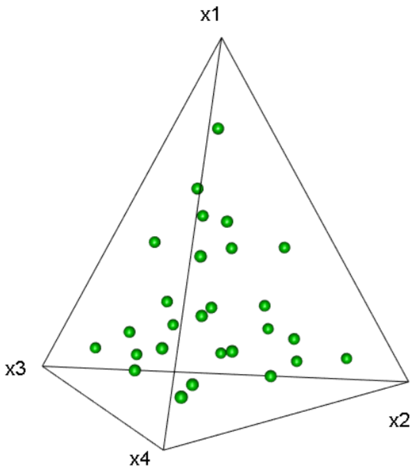
Example 4.

Now, we illustrate the results of the above discussion by taking the pseudo-component transformations of the 3-component second-order lattice point set. As shown in Figure 2, Equation (10) holds wherever the test point falls into the region.

We note that it is more complicated in the case of a sub-simplex partitioned by a lattice point set for $q>4$. However, by calculation, we find that the uniformity of the point set is best for the lattice point set transformed by the pseudo-component with the center point as the reference, and when the transformation parameters are equal to the order of the lattice points.

Suppose that the mixture region $S^{q-1}$ is partitioned by $\mathcal{L}\{q,m\}$ into n sub-simplexes $S^{q-1}=V_1+V_2+\cdots +V_n$ with no common interior point. For any point $\mathbf{x}\in \mathcal{X}$, there must exist a sub-simplex $V_i=V_i\left\{{\mathbf{x}}_{i1},{\mathbf{x}}_{i2},\cdots ,{\mathbf{x}}_{iq}\right\}$, such that $\mathbf{x}\in V_i$. Further, for a single point design $\mathcal{P}=\left\{\mathbf{x}\right\}$, where $\mathbf{x}\in V_i$. Then, the uniform design satisfying the MD-uniform criterion on the simplex region can be constructed by the lattice partition design when

$$\underset{\mathbf{x}\in V_i}{arg}\mathrm{md}\left(\mathcal{P}\right)=\underset{\mathbf{x}\in {\mathrm{V}}_{\mathrm{i}}}{arg}\underset{{\mathbf{t}}_{\mathrm{k}}\in {\mathrm{V}}_{\mathrm{i}}}{max}\left\{{\mathrm{d}}^2({\mathbf{t}}_{\mathrm{k}},{\mathcal{P}}_{\mathrm{n}})\right\}={\mathbf{x}}_{\mathrm{i}0}=\frac{1}{\mathrm{q}}\sum _{\mathrm{j}=1}^{\mathrm{q}}{\mathbf{x}}_{\mathrm{ij}}.$$

Therefore, the design obtained from partitioning a simplex using a lattice point set should satisfy the MD-uniform criterion if the centroid of each sub-simplex is taken as the design point.

5. Uniform Test on the Mixture Region

As mentioned above, the lattice point set is used to partition the simplex $S^{q-1}$. We note that some sub-regions are composed of multiple sub-simplexes, while other sub-domains are only sub-simplex. In large-sample surveys, it is necessary to check whether the samples are evenly distributed on the simplex. In this section, we mainly provide the uniform test method on the mixture region.

Suppose that $\mathcal{X}$ is a mixture region, and $V_i,i=1,2,\cdots ,k$ is an arbitrary partition of $\mathcal{X}$. From the result in Section 3, $\mathcal{X}={\displaystyle \sum _{i=1}^k}{V}_i$ and there is no common interior point between two simplexes $V_i$ and $V_j$, where $V_i=V_i\{{\mathbf{x}}_{i1}{,\mathbf{x}}_{i2},\cdots {,\mathbf{x}}_{iq}\},i=1,2,\cdots ,k,i\ne j$.

Now, for the point set ${\mathcal{P}}_N=\{{\mathbf{x}}_1,{\mathbf{x}}_2,\cdots ,{\mathbf{x}}_N\}\subset \mathcal{X}\subseteq S^{q-1}$, let

$$N_{V_i}=card\{{\mathcal{P}}_N\cap V_i\},i=1,2,\cdots ,k$$

be the number of points in $V_i$ containing ${\mathcal{P}}_N$. We denote

$$\begin{array}{c}\hfill \mathrm{AD}\left({\mathcal{P}}_{\mathrm{N}}\right)=\frac{1}{\mathrm{k}}\sum _{\mathrm{i}=1}^{\mathrm{k}}{\left(\frac{{\mathrm{N}}_{{\mathrm{V}}_{\mathrm{i}}}}{\mathrm{N}}-\frac{\mathrm{Vol}({\mathrm{V}}_{\mathrm{i}})}{\mathrm{Vol}(\mathcal{X})}\right)}^2.\end{array}$$

(11)

Note that AD$\left({\mathcal{P}}_N\right)$ is a function of $\frac{N_{V_i}}{N}$ and it can be used to measure the uniformity of ${\mathcal{P}}_N$ on the mixture region $\mathcal{X}$. If ${\mathcal{P}}_N$ distributes uniformly in the experimental region $\mathcal{X}$, this means that AD$\left({\mathcal{P}}_N\right)$ will be as small as possible.

We denote $p_i=\frac{\mathrm{Vol}\left(V_i\right)}{\mathrm{Vol}\left(\mathcal{X}\right)}$ as the volume ratio of sub-simplex $V_i$ to mixture region $\mathcal{X}$; let

$${\widehat{p}}_i=\frac{N_{V_i}}{{\displaystyle \sum _{i=1}^k}{N}_{V_i}}$$

be the proportion of the number of points in $V_i$.

If the points are distributed uniformly in mixture region $\mathcal{X}$, then the $\frac{N_{V_i}}{N}$ will be the unbiased estimation of $\frac{\mathrm{Vol}\left(V_i\right)}{\mathrm{Vol}\left(\mathcal{X}\right)}$.

In order to test whether ${\mathcal{P}}_N$ is distributed uniformly on the mixture region, the null hypothesis “$H_0:{\mathcal{P}}_N$ distributed uniformly in the region $\mathcal{X}$ ” can be considered. Then, the test statistic is

$$\begin{array}{c}\hfill {\chi }^2=N\sum _{i=1}^k\frac{{\left({\widehat{p}}_i-p_i\right)}^2}{p_i(1-p_i)}.\end{array}$$

(12)

Now, if the null hypothesis $H_0$ is held, then ${\chi }^2\sim {\chi }^2\left(k\right)$. When the significant value $p^{*}=P({\chi }^2>{\chi }^2\left(k\right))<0.05$ (or $0.01$), we reject the null hypothesis $H_0$.

In particular, if the volumes of sub-simplex $V_i,i=1,2,\cdots ,k$ obtained by the partition of the lattice point sets are approximately equal, that is $\frac{\mathrm{Vol}\left(V_i\right)}{\mathrm{Vol}\left(\mathcal{X}\right)}\approx p,i=1,2,\cdots ,k,$ we have

$${\chi }^2=\frac{N}{p(1-p)}\sum _{i=1}^k{\left({\widehat{p}}_i-p\right)}^2.$$

Therefore, if the null hypothesis $H_0$ is held, we have

$${\chi }^2=\frac{Nk\mathrm{AD}\left({\mathcal{P}}_{\mathrm{N}}\right)}{p(1-p)}\dot{\sim }{\chi }^2\left(k\right).$$

Furthermore, the 0.95 two-side confidence intervals of $\mathrm{AD}\left({\mathcal{P}}_{\mathrm{N}}\right)$ can be given by

$$\begin{array}{c}\hfill \left[\frac{p(1-p)}{Nk}{\chi }_{0.025}^2\left(k\right),\frac{p(1-p)}{Nk}{\chi }_{0.975}^2\left(k\right)\right].\end{array}$$

(13)

Next, we will partition the simplex by the lattice point set and provide the steps of the uniformity test as follows.

Step 1. From the result in Section 3, we obtain r sub-regions $S_{\left[{\mathbf{a}}_j{,\mathbf{b}}_j\right]}^{q-1}$ without a common interior point by using m order lattice point set to partition the simplex $S^{q-1}$, as shown in (8).

Step 2. Since the number of extreme vertices for the sub-region $S_{\left[{\mathbf{a}}_j{,\mathbf{b}}_j\right]}^{q-1}$ is greater than q, then it can be partitioned into $k(k\ge r)$ sub-simplexes $V_1,V_2,\cdots ,V_k$.

Step 3. Suppose that ${\mathcal{P}}_N=\{{\mathbf{x}}_1,{\mathbf{x}}_2,\cdots ,{\mathbf{x}}_N\}\subset S^{q-1}$ are tested samples, and $P_N=\left[{\mathbf{x}}_1,{\mathbf{x}}_2,\cdots ,{\mathbf{x}}_N\right]$$={\left\{x_{ji}\right\}}_{i,j=1}^{q,N}$ is a matrix array as row by the N points. Let ${\mathbf{V}}_i^{-1}{P}_N=\left[{\mathit{\alpha }}_1^i,{\mathit{\alpha }}_2^i,\cdots ,{\mathit{\alpha }}_N^i\right]={\left\{{\alpha }_{uv}^i\right\}}_{u,v=1}^{q,N}$, and we have

$$N_{V_i}=card\{{\mathcal{P}}_N\cap V_i\}=\sum _{v=1}^N\left[\prod _{u=1}^{q}I(0<{\alpha }_{uv}^i<1)\right],i=1,2,\cdots ,k.$$

Step 4. Calculate the value of the test statistic result and the confidence interval by using (11).

We note that the partitioning of a simplex $S^{q-1}$ by the lattice point set method not only provides a uniformity test but also constructs a pseudo-component transformation in the sub-simplex. Moreover, it obtains a design that is uniformly distributed in the simplex.

For example, let ${\mathbf{x}}_i^0$ be the centroid point in the sub-simplex $V_i$ and take ${\mathbf{x}}_i^0$ as the reference point. Using the pseudo-component transformation method to convert the vertices of $V_i$ will enable each sub-simplex to contain q interior points and the design to contain $q{m}^{q-1}$ experimental points. However, the design constructed by this method will face the problem of “dimensional disaster” when q is larger. To reduce the number of experiments, we consider taking the center of the sub-simplex of each partition. Then, the design will only contain $m^{q-1}$ experimental points in total. Moreover, if the experiments are arranged with a set of higher-order lattice points, when $q>4,m>4$, the number of sub-simplexes is larger than the number of a lattice point set. Further, since the convex polyhedron can be partitioned into several disjoint sub-regions, as shown in (8), then the centroid of each sub-region will be evenly distributed on the experimental region.

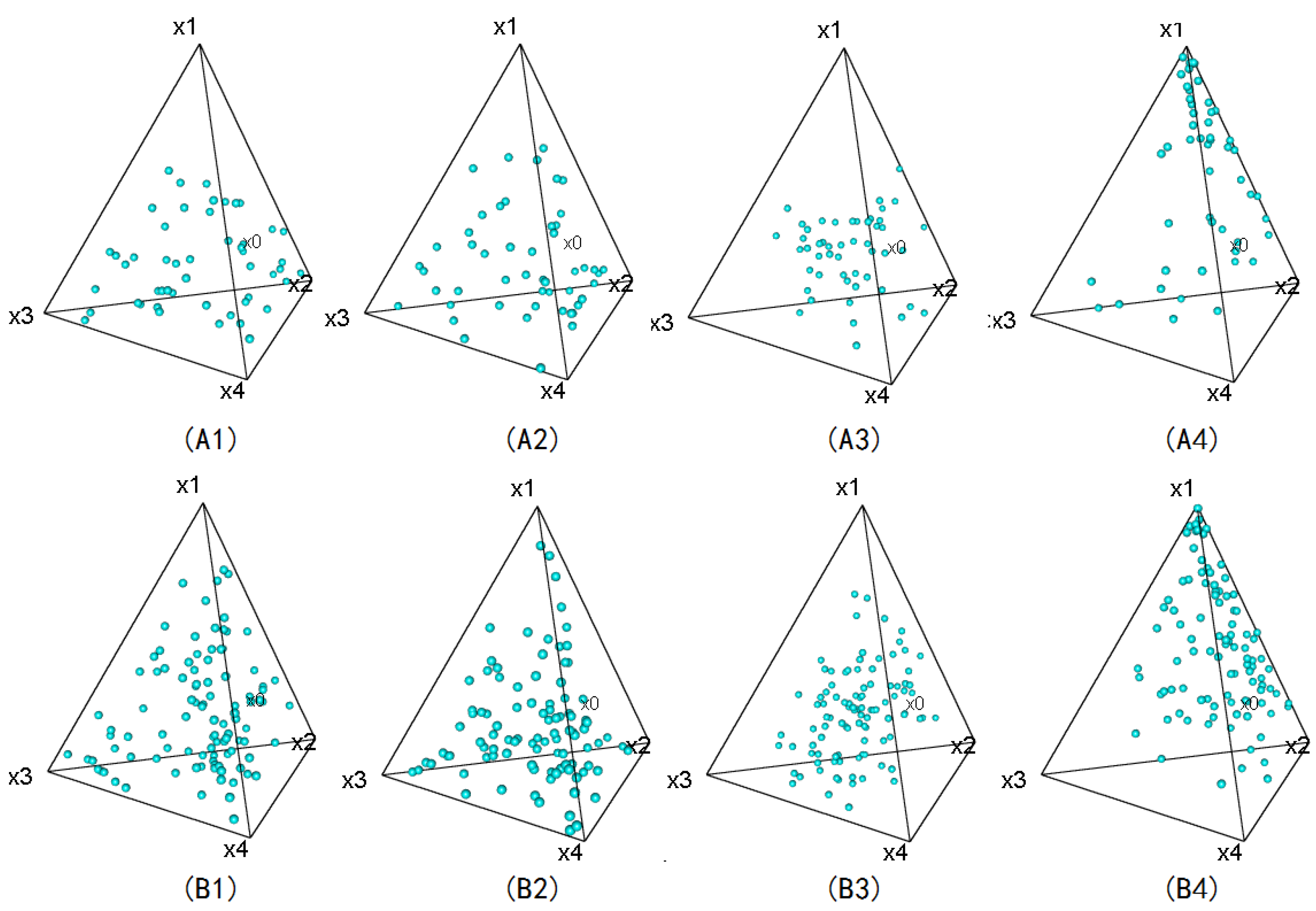
In order to compare the results of the uniform test, we provide four different methods to generate random points in a simplex. We first generate a random matrix $Y={\left\{y_{ij}\right\}}_{i,j=1}^{N,q}$, where $y_{ij}\sim U\left(0,1\right),i=1,2,\cdots ,N,j=1,2,\cdots ,q$, and each $y_{ij}$ is independent. Suppose that $N\gg n$; then, the matrix $T={\left\{x_{ij}\right\}}_{i,j=1}^{N,q}$ can be obtained by an inverse transformation of the matrix Y.

(1) Exponential transformation method

The exponential transformation method was proposed by Fang and Wang (1994) [4], where each element of T can be calculated by

$$x_{ij}=\frac{log\left(1-y_{ij}\right)}{{\displaystyle \sum _{j=1}^q}log\left(1-y_{ij}\right)},i=1,2,\cdots ,N,j=1,2,\cdots ,q.$$

(14)

(2) Inverse transformation method

Another alternative is the inverse transform method introduced by Fang and Wang (1996) [5], where the elements of T can be calculated by

$$\begin{array}{c}\hfill \left\{\begin{array}{c}{x}_{ij}=\left(1-y_{ij}^{1/\phantom{1(q-j)}(q-j)}\right){\displaystyle \prod _{l=1}^{j-1}}{y}_{il}^{1/\phantom{1(q-l)}(q-l)},j=1,2,\cdots ,q-1,\hfill \\ x_{iq}={\displaystyle \prod _{l=1}^{q-1}}{y}_{il}^{1/\phantom{1(q-l)}(q-l)},i=1,2,\cdots ,N.\hfill \end{array}\right.\end{array}$$

(15)

Let ${\mathbf{x}}_i=(x_{i1},x_{i2},\cdots ,x_{iq})$ be the i-th row in matrix T, which is inversely transformed by (14) or (15). Then, each row element of T satisfies

$${\mathbf{x}}_i\sim U\left(S^{q-1}\right),\sum _{j=1}^q{x}_{ij}=1,i=1,2,\cdots ,N$$

and ${\mathbf{x}}_1,{\mathbf{x}}_2,\cdots ,{\mathbf{x}}_N$ are independent of each other. Therefore, the elements ${\mathbf{x}}_1,{\mathbf{x}}_2,\cdots ,{\mathbf{x}}_N$ of T can be used as a randomly generated experimental point on the simplex $S^{q-1}$. Next, we provide the other two methods as follows.

(3) Method I

Suppose that $X_i,i=1,2,\cdots ,q$ is an independent and identically distributed nonnegative random variable and $X_i\stackrel{i.i.d}{\sim }{F}_X\left(x\right)$. Let

$$\begin{array}{c}\hfill Y_i=\frac{X_i}{{\displaystyle \sum _{i=1}^q}{X}_i},i=1,2,\cdots ,q,\end{array}$$

(16)

and then each of $\mathbf{Y}={(Y_1,Y_2,\cdots ,Y_q)}^{\mathrm{T}}$ is a random mixture point on the $q-1$-dimensional simplex, and note that the distribution of $\mathbf{Y}={(Y_1,Y_2,\cdots ,Y_q)}^{\mathrm{T}}$ is determined by each random variable $X_i,i=1,2,\cdots ,q$.

(4) Method II

Suppose that the random variable $X_1\sim U(0,1)$, and let

$$X_2\sim U(0,1-X_1),\cdots ,X_{q-1}\sim U(0,1-\sum _{j=1}^{q-2}{X}_j),X_q=1-\sum _{j=1}^{q-1}{X}_j.$$

Then, $\mathbf{Z}={(X_1,X_2,\cdots ,X_q)}^{\mathrm{T}}$ is also a random mixture point on the $q-1$-dimensional simplex.

6. Illustrative Examples

In this section, we will provide two examples to illustrate that the method proposed in Section 3 for constructing a uniform design is feasible and the random mixture points are effective for uniform tests on the simplex as proposed in Section 5.

Example 5.

Suppose that the 20 design points in $\mathcal{L}\{4,3\}$ are as follows.

$$\begin{array}{cccc}{\mathbf{x}}_1=\left(1,0,0,0\right),\hfill & {\mathbf{x}}_2=\left(\frac{2}{3},\frac{1}{3},0,0\right),& {\mathbf{x}}_3=\left(\frac{1}{3},\frac{2}{3},0,0\right),& {\mathbf{x}}_4=\left(0,1,0,0\right),\\ {\mathbf{x}}_5=\left(\frac{2}{3},0,\frac{1}{3},0\right),\hfill & {\mathbf{x}}_6=\left(\frac{1}{3},\frac{1}{3},\frac{1}{3},0\right),& {\mathbf{x}}_7=\left(0,\frac{2}{3},\frac{1}{3},0\right),& {\mathbf{x}}_8=\left(\frac{1}{3},0,\frac{2}{3},0\right),\\ {\mathbf{x}}_9=\left(0,\frac{1}{3},\frac{2}{3},0\right),\hfill & {\mathbf{x}}_{10}=\left(0,0,1,0\right),& {\mathbf{x}}_{11}=\left(\frac{2}{3},0,0,\frac{1}{3}\right),& {\mathbf{x}}_{12}=\left(\frac{1}{3},\frac{1}{3},0,\frac{1}{3}\right),\\ {\mathbf{x}}_{13}=\left(0,\frac{2}{3},0,\frac{1}{3}\right),\hfill & {\mathbf{x}}_{14}=\left(\frac{1}{3},0,\frac{1}{3},\frac{1}{3}\right),& {\mathbf{x}}_{15}=\left(0,\frac{1}{3},\frac{1}{3},\frac{1}{3}\right),& {\mathbf{x}}_{16}=\left(0,0,\frac{2}{3},\frac{1}{3}\right),\\ {\mathbf{x}}_{17}=\left(\frac{1}{3},0,0,\frac{2}{3}\right),\hfill & {\mathbf{x}}_{18}=\left(0,\frac{1}{3},0,\frac{2}{3}\right),& {\mathbf{x}}_{19}=\left(0,0,\frac{1}{3},\frac{2}{3}\right),& {\mathbf{x}}_{20}=\left(0,0,0,1\right).\end{array}$$

Then, from the result in (8), the $S^{q-1}$ can be partitioned into 15 sub-regions $S_{\left[{\mathbf{a}}_j{,\mathbf{b}}_j\right]}^{4-1}$ under $\mathcal{L}\{4,3\}$ and $S^{q-1}=S_{\left[{\mathbf{a}}_j{,\mathbf{b}}_j\right]}^{4-1},j=1,2,\cdots ,15.$ The vector of lower constraints (VLC) and the vector of upper constraints (VUC) are given in column 2 and column 3 in

Table 1. Partition of $S^{4-1}$ under the $\mathcal{L}\{4,3\}$.

NO.	VLC	VUC	Vertex Sets				Volume $\times {10}^2$	Centroid
1	$(0,0,0,0)$	$(\frac{1}{3},\frac{1}{3},\frac{1}{3},\frac{1}{3})$	6	12	14	15	1.230868	$(0.2498,0.2498,0.2498,0.2498)$
2			2	6	12	14	1.233640	$(0.4165,0.2498,0.1665,0.1665)$
3			2	5	11	14	1.233640	$(0.5835,0.0833,0.1665,0.1665)$
4	$(\frac{1}{3},0,0,0)$	$(\frac{2}{3},\frac{1}{3},\frac{1}{3},\frac{1}{3})$	2	5	6	14	1.233640	$(0.5000,0.1665,0.2498,0.0833)$
5			2	11	12	14	1.233640	$(0.5000,0.1665,0.0833,0.2498)$
6	$(\frac{2}{3},0,0,0)$	$(1,\frac{1}{3},\frac{1}{3},\frac{1}{3})$	1	2	5	11	1.230868	$(0.7503,0.0833,0.0833,0.0833)$
7			3	7	13	15	1.233640	$(0.0833,0.5835,0.1665,0.1665)$
8	$(0,\frac{1}{3},0,0)$	$(\frac{1}{3},\frac{2}{3},\frac{1}{3},\frac{1}{3})$	3	6	12	15	1.233640	$(0.2498,0.4165,0.1665,0.1665)$
9			3	6	7	15	1.233640	$(0.1665,0.5000,0.2498,0.0833)$
10			3	12	13	15	1.233640	$(0.1665,0.5000,0.0833,0.2498)$
11	$(\frac{1}{3},\frac{1}{3},0,0)$	$(\frac{2}{3},\frac{2}{3},\frac{1}{3},\frac{1}{3})$	2	3	6	12	1.236418	$(0.4165,0.4165,0.0833,0.0833)$
12	$(0,\frac{2}{3},0,0)$	$(\frac{1}{3},1,\frac{1}{3},\frac{1}{3})$	3	4	7	13	1.230868	$(0.0833,0.7503,0.0833,0.0833)$
13			8	9	15	16	1.233640	$(0.0833,0.1665,0.5835,0.1665)$
14	$(0,0,\frac{1}{3},0)$	$(\frac{1}{3},\frac{1}{3},\frac{2}{3},\frac{1}{3})$	6	8	14	15	1.233640	$(0.2498,0.1665,0.4165,0.1665)$
15			6	8	9	15	1.233640	$(0.1665,0.2498,0.5000,0.0833)$
16			8	14	15	16	1.233640	$(0.1665,0.0833,0.5000,0.2498)$
17	$(\frac{1}{3},0,\frac{1}{3},0)$	$(\frac{2}{3},\frac{1}{3},\frac{2}{3},\frac{1}{3})$	5	6	8	14	1.236418	$(0.4165,0.0833,0.4165,0.0833)$
18	$(0,\frac{1}{3},\frac{1}{3},0)$	$(\frac{1}{3},\frac{2}{3},\frac{2}{3},\frac{1}{3})$	6	7	9	15	1.236418	$(0.0833,0.4165,0.4165,0.0833)$
19	$(0,0,\frac{2}{3},0)$	$(\frac{1}{3},\frac{1}{3},1,\frac{1}{3})$	8	9	10	16	1.230868	$(0.0833,0.0833,0.7503,0.0833)$
20			15	17	18	19	1.233640	$(0.0833,0.1665,0.1665,0.5835)$
21	$(0,0,0,\frac{1}{3})$	$(\frac{1}{3},\frac{1}{3},\frac{1}{3},\frac{2}{3})$	12	14	15	17	1.233640	$(0.2498,0.1665,0.1665,0.4165)$
22			12	15	17	18	1.233640	$(0.1665,0.2498,0.0833,0.5000)$
23			14	15	17	19	1.233640	$(0.1665,0.0833,0.2498,0.5000)$
24	$(\frac{1}{3},0,0,\frac{1}{3})$	$(\frac{2}{3},\frac{1}{3},\frac{1}{3},\frac{2}{3})$	11	12	14	17	1.236418	$(0.4165,0.0833,0.0833,0.4165)$
25	$(0,\frac{1}{3},0,\frac{1}{3})$	$(\frac{1}{3},\frac{2}{3},\frac{1}{3},\frac{2}{3})$	12	13	15	18	1.236418	$(0.0833,0.4165,0.0833,0.4165)$
26	$(0,0,\frac{1}{3},\frac{1}{3})$	$(\frac{1}{3},\frac{1}{3},\frac{2}{3},\frac{2}{3})$	14	15	16	19	1.236418	$(0.0833,0.0833,0.4165,0.4165)$
27	$(0,0,0,\frac{2}{3})$	$(\frac{1}{3},\frac{1}{3},\frac{1}{3},1)$	17	18	19	20	1.230868	$(0.0833,0.0833,0.0833,0.7503)$

, respectively. In these sub-regions, there exist some regions that cannot be further partitioned, shown in Table 1, row $1,6,11,12,17,18,19,25,26,27.$ Moreover, there also exist some sub-regions composed of four sub-simplexes, shown in Table 1, row 2–5, 7–10, 13–16 and 20–23. Next, we can obtain the sub-simplex for these sub-regions by further partitioning.

Therefore, the simplex $S^{4-1}$ be partitioned into 27 sub-simplexes without common interior points under the 20 design points of $\mathcal{L}\{4,3\}$. The order number of four vertexes for each sub-simplex corresponds to the design point of $\mathcal{L}\{4,3\}$. For example, the four vertexes ${\mathbf{x}}_6,{\mathbf{x}}_{12},{\mathbf{x}}_{14},{\mathbf{x}}_{15}$ of sub-simplex are composed of the vector of lower constraints ${\mathbf{a}}_{\mathbf{1}}=(0,0,0,0)$ and the vector of upper constraints ${\mathbf{b}}_{\mathbf{1}}=(\frac{1}{3},\frac{1}{3},\frac{1}{3},\frac{1}{3})$. By calculation, we find that there exist differences among the volumes of these sub-simplexes, but the error is less than ${10}^{-4}$. Moreover, the distribution of the centroid for these sub-simplexes is shown in Figure 3, and the values of these centroid and each sub-simplex are shown in Table 1.

Example 6.

Now, we use the inverse transformation method and the exponential inverse transformation method, method I and method II to generate $N=50$ and $N=100$ random mixing points, respectively.

Take $X_i\stackrel{i.i.d.}{\sim }U(0,1),i=1,2,\cdots ,q$ in (16). The distribution of random points in various cases is as shown in Figure 4.

Note that (A1), (A2), (A3) and (A4) are the distribution of 50 random mixture points generated by the inverse and exponential inverse transformation methods, method I and method II, respectively. (B1), (B2), (B3) and (B4) are the distributions of 100 random mixing points produced by the four methods, respectively. Next, we will compare the uniformity distribution of the random mixture points generated by these four methods and test it. As shown in Example 5, using the lattice point set $\mathcal{L}\{4,3\}$, the simplex $S^{4-1}$ can be partitioned into 27 sub-simplexes. The volumes and centroid of each sub-simplex are shown in Table 1. Then, the values of the uniformity test for the four methods with $N=50$ and $N=100$ are shown in the following

Table 2. The uniformity test of random mixture point set generated by four methods.

Number of Samples	Method	$\mathbf{AD}\left({\mathcal{P}}_{\mathbf{N}}\right)$	${\mathit{\chi }}^2$	${\mathit{p}}^{*}$
	Exponential inverse transformation	0.000733	27.73904	0.424521
$N=50$	Inverse transformation method	0.000584	22.1094	0.731798
	Method I	0.004882	185.0917	<0.01
	Method II	0.002213	83.80955	<0.01
	Exponential inverse transformation	0.000488	36.95872	0.095841
$N=100$	Inverse transformation method	0.000377	28.51026	0.385039
	Method I	0.003288	249.2317	<0.01
	Method II	0.000850	64.38735	<0.01

. From the result of the uniformity test, we find that both the significant values $p^{*}<0.01$ for method I and method II. Therefore, it is necessary to reject the null hypothesis $H_0$, and the random mixture points generated by the exponential inverse transformation and inverse transformation method have a uniform distribution on the $S^{4-1}$.

7. Conclusions

Lattice point sets are a critical tool for constructing uniform designs for experiments with mixtures. Using a lattice point set to partition the irregular mixture regions, the sum of the volume for each partitioned sub-simplex is approximately equal to the volume of the mixture region. In addition, if there is a mixture experimental region with upper and lower bound constraints, then the sum of the volumes of the sub-simplex, obtained by using the lattice point set for partitioning, is precisely equal to the volume of the constrained experimental region.

In this paper, we propose a method of partitioning for mixture regions, obtaining several sub-simplexes without common interior points, which are important for constructing uniform designs. Furthermore, under the partition of the lattice point set, we construct the statistical uniform test on the simplex by using the ratio of volume between the sub-simplex and mixture region. We find that the random mixture points generated by the exponential inverse transformation and inverse transformation method are distributed uniformly in the mixture region.

Currently, there exist relevant results on the division of lattice point sets for low-dimensional mixture simplexes without additional constraints. However, the algorithms for the approximate partitioning of high-dimensional and mixture experimental regions with additional constraints have not been improved. Moreover, there are two primary aspects for further studies: on the one hand, developing a complete theoretical system for the partitioning of lattice point sets in high-dimensional experimental regions with upper and lower bound constraints, linear constraints and additional non-linear constraints; on the other hand, it is necessary to algorithmically implement irregular region dissection, where the partition is unique when the number of components and the order of lattice points are determined.