Abstract
This article is a study of vector-valued renewal-reward processes on . The jumps of the process are assumed to be independent and identically distributed nonnegative random vectors with mutually dependent components, each of which may be either discrete or continuous (or a mixture of discrete and continuous components). Each component of the process has a fixed threshold. Operational calculus techniques and symmetries with respect to permutations are used to find a general result for the probability of an arbitrary weak ordering of threshold crossings. The analytic and numerical tractability of the result are demonstrated by an application to the reliability of stochastic networks and some other special cases. Results are shown to agree with empirical probabilities generated through simulation of the process.
1. Introduction
Analysis of sums of independent random variables falls into the classical theory of fluctuations, which has been widely studied, from fluctuations about thresholds [1,2,3,4] to ruin times to limiting distributions [5,6] and bounds [7], but less frequent are studies of sums of independent random vectors. Most development is in the areas of limit theorems and other asymptotic results [8,9,10,11].
More infrequent are studies of the threshold crossings of sums of independent random vectors, which may be considered in the context of multidimensional renewal processes [12,13] or random walks [14,15]. Most of these tend to focus on exit times [16,17,18,19,20] and overshoots of the boundary [21,22]. These latter ideas are commonly studied in the context of broader Lévy processes as well [23,24,25], but frequently only in one dimension. Another recent and interesting work [26] provides some analysis of fluctuations of the more general idea of spectrally positive additive Lévy fields.
Studies in these areas have broad applications, including works applied to insurance [27,28,29], finance [30,31,32], stochastic games [33,34], queueing theory [35,36,37], and reliability theory [38,39], among other fields.
1.1. Goals and Structure of the Paper
This paper focuses on a different, but related question: if there is a threshold in each dimension, i.i.d. sums of nonnegative random vectors (not strictly 0) will almost surely cross them all eventually, but what is the probability that the thresholds are crossed in a specific (weak) order?
After giving the mathematical setting for the problem in Section 1.2 and establishing some lemmas in Section 2, we derive a formula for the probabilities through operational calculus techniques and symmetries with respect to permutations in Section 3 to answer this question. In Section 4, the formulas are shown to be analytically tractable in an application to the reliability of stochastic networks and numerically tractable in a three-dimensional problem, and all are shown to agree with simulated results for special cases. In Section 5, we describe how the results herein fall into a wider project and should contribute to some forthcoming results.
1.2. The Mathematical Setting of the Problem
On a probability space , consider a sequence of i.i.d. nonnegative real random vectors with such that each has a common Laplace–Stieltjes transform
where such that each component of x has a nonnegative real part. We also assume for each k.
Note that while the random vectors , , … are independent, we make no such assumption on the components of , so may have some arbitrary dependency structure.
Consider a renewal-reward process
where forms a renewal process of jump times. Since we are concerned only with the crossing order, studying the renewal-reward process directly is unnecessary, so we can focus on the embedded discrete-time stochastic process
with the marginal processes
and the approach and crossing of fixed thresholds in each coordinate.
In other words, we are interested in the first n such that for each k, i.e., the first time each coordinate crosses its fixed threshold .
Denote the first crossing index of the threshold of the kth coordinate as
Each can be viewed as the first time when the process exits .
We will derive the probability of an event W, a fixed weak ordering of the threshold crossings , …, . In other words, W is an element of the following measurable partition of the sample space ,
where, in each event, each relation is fixed to be < or = for some fixed permutation p of the dimensions .
We will assume that p is the identity function. Since the probability will be shown to be symmetric with respect to permutations of the threshold crossings in the main result of the paper, Theorem 1. Hence, the results trivially follow for arbitrary weak ordering.
It should be noted that deriving results about the crossing times, positions, or excess levels of the underlying renewal-reward process would require further information about the jump times . However, much prior scholarship by Takács [3,4] classically, and by Dshalalow and his collaborators over the past few decades, demonstrates that results about crossing weak orders of the embedded discrete-time process easily extend to results about the crossing times and position of renewal-reward processes [12], as well as monotone [14,30] and even oscillating [15] marked random walks. However, all such prior works were limited to, at most, four dimensions. The present work generalises these ideas to arbitrary finite dimension.
2. Preliminary Results
We need to establish two lemmas before proving the main result. First, a simple algebraic lemma is established.
Lemma 1.
For a vector ,
where
where the sum runs over all k-subsets of , each denoted , and we define .
Proof.
We will first establish some properties of the function and then prove the lemma via induction on d.
Notice that is the sum of all -factor products from , so, if this is multiplied by , we have the sum of all k-factor products from including as a factor. Note that is the sum of all k-factor products from or, equivalently, the sum of all k-factor products of terms from not including as a factor. Adding them,
Further, since there is exactly one product of n distinct terms from , we have
Let ; then, the left side of (7) is while the right side is
Suppose that, for , it is true that
then, for , we have
Rearranging the sums,
By (8) and (9) and the fact that ,
Thus, the result of the lemma is true by induction. □
Second, we establish a minor sufficient condition under which , where is the joint Laplace–Stieltjes transform of the i.i.d. random vectors introduced in (1). This is required later for summing as a geometric series.
Lemma 2.
If any component of x has a positive real part, then .
Proof.
Note that
Since each is real and nonnegative and each by assumption, each exponential term is in , so, for any , this implies
Suppose that we partition into and ; then,
If , then , so we have
If , this result implies merely , but if , it implies , recalling by assumption. Since j was arbitrary, we have if at least one component of x has a positive real part. □
With these preliminary results established, we continue towards proving the main result of the paper.
3. The Main Result
In this section, we derive for an arbitrary weak ordering . Regardless of W, the exit indices must occur at some distinct times since some may occur simultaneously.
Without loss of generality, we can suppose that the groups of simultaneous crossing indices are
and . The values are, then, the number of crossing indices in the first k groups. (Note that, the subscripts may actually occur with some permutation p of the given subscripts, so we may easily replace with given p.)
Further, denote as the number of crossing indices in the kth group. Then, we can represent an arbitrary weak ordering W as
We will partition W into events of the form
where j is such that , and is a vector of thresholds in each dimension to be used during some intermediate steps of the upcoming proofs. As such, the threshold function equals the true for each .
To be precise, an operator to be defined next will be applied to for an arbitrary fixed q vector and summed over all permissible j vectors to derive , where
under the operator. The inverse operator will then be applied at the true threshold vector to reconstruct the desired probability .
We will use an operator defined as
which is a composition of d operators, one for each component of the process . The operators take one of two forms, depending on whether the corresponding component is discrete or continuous,
where is the Laplace–Carson transform,
defined for nonnegative measurable functions f and . D is defined as
for functions f and . This operator has the inverse
Since each operator can reconstruct , note that using will allow us to reconstruct f evaluated at . This is important for the main result of the paper, Theorem 1, so that we can derive the probabilities for the proper threshold values , …, .
We see that D is similar to a z-transform and has been used in more or less the same way for discrete problems as variants of the Laplace transforms have been used for continuous problems in stochastic processes. Common use of such operators be found frequently in, for example, many earlier works of Takács [3,4,35] and Dshalalow and his collaborators [12,40].
Before deriving , we need to establish one last lemma.
Lemma 3.
For an event , suppose that each for each ; then,
where
and
Proof.
If a component is continuous, note simply that
If a component is discrete, similarly, we can sum as two partial geometric series,
Denote for with and . Further, for and each , define where and denote
so that we may refer to the joint transform of a specific subset of the random variables making up the random jump vectors .
Given the lemmas above, we may derive as an expression in terms of inverse of the operator and the common joint transform of the random vectors as follows.
Theorem 1.
If each vector contains at least one component with a positive real part, then, for each ,
Proof.
Without loss of significant generality, assume that is continuous in each component. A remark after the proof will show how the result generalises to accommodate processes with some discrete components. To find , we merely need to sum the probabilities of the events , which partition W, as follows.
Next, apply the operator, which bypasses all terms except the q-dependent indicator,
Then, by Lemma 3, we have
Since the vectors are i.i.d.,
Notice that the expression above has n nested infinite series, which fall into two types. First, in (28) and (29), the first series are identical except for the subscripts. The last series in (30) is slightly different because . We will consider (28) in detail, and the other two cases follow by nearly the same argument.
Notice that (28) has two expectations. Since the vectors are i.i.d., the first expectation simplifies to , yielding
If we set , Lemma 1 implies that the above may be written as
which may be simplified as
Note that the last sum is constant with respect to . Since has a component with a positive real part, Lemma 2 implies , so the infinite series is a geometric series, so the above simplifies to
Through a very similar argument but with different indices, the terms of the form (29) and (30) simplify to
Plugging (34) and (35) into (28)–(30) gives
Applying the inverse operator evaluated at yields (24), the claim of the theorem. □
Note that, without exploiting the symmetry of the argument above with respect to permutations, the proof would have been infeasible since one would have to consider each permutation of threshold crossing indices and render a separate argument. Since the number of permutations grows factorially with dimension, prior multivariate results were limited to [12] or at most [30].
Remark 1.
For convenience, the proof above was rendered under the assumption that the components of are continuous-valued. However, for any discrete component of the process, , replacing the corresponding with and replacing with
and maintaining all other steps of the proof yields the same result.
Example 1.
Suppose that ; then, we have
so and . Then, Theorem 1 implies
If γ is known, the operators may be inverted one-by-one to find a tractable expression for the probability, as we demonstrate with several models in the next section.
Suppose a similar weak ordering W where the permutation
has been applied to the threshold numbers. Then, the weak ordering is
By Theorem 1 and referring to (39), the result is trivially found to be
The symmetry of the result with respect to permutations makes this the same as (39) but for the application of the permutation p to the dimension numbers.
4. Applications and Special Case Results
In this section, we apply Theorem 1 to find probabilities of weak orderings of threshold crossings in a problem associated with the reliability of stochastic networks, as well as two special cases of random vectors with exponential distributions.
Any exact Laplace transform inversions in this section are computed using sequences of tabled results from Supplement 5 of [41] or with Wolfram Mathematica. In Section 4.3, some results require numerical inverse Laplace transforms rendered via methods developed from the Talbot algorithm [42]. In particular, we use McClure’s MATLAB implementation [43] following the unified framework of Abate and Whitt [44].
Inverse transforms will be evaluated in exact form using properties derived by Dshalalow and summarized in Appendix B of [45]. Many of the results have been used to invert the operator in works from Dshalalow and his collaborators [36,46,47].
In each application and special case below, the processes are further simulated in MATLAB to find empirical probabilities, which are shown to match the numerical and analytic results derived from inverting the sequences of operators.
4.1. Application to Stochastic Networks
Some prior work [38,39,45] studies processes that model stochastic networks under attack, where successive batches of nodes of random size are incapacitated upon a Poisson point process on , where each node has random weight measuring its value to the network. In these works, most attention was given to a ruin time where cumulative node loss crosses a threshold or cumulative weight loss crosses another threshold , whichever comes first. This ruin time represents the network entering a critical state of interest. Probabilistic information about this time and the extent of different types of damage that should be anticipated in the near term can give security professionals earlier warnings of attacks and help them to differentiate malicious attacks from benign failures on the network.
While understanding the timing and extent of critical damage is important, it leaves network administrators with more new questions than answers: What should we do about different attack patterns? Where are our weaknesses?
The present work can address is the probability of each ordering of failures, which would indicate the more vulnerable part of the network, whether nodes or weights, which can suggest strategies for improving reliability.
To model the situation, suppose that each jump in the process is a vector consisting of the batch size and sum of weights . Since each node weight is ,
where we assume that the node batch sizes are i.i.d. with common probability-generating function g and the weights are i.i.d. with common Laplace–Stieltjes transform l.
We will seek to apply Theorem 1 to find the probabilities of each weak ordering of threshold crossings, which requires knowledge of , which we can find by double expectation,
Corollary 1.
If node batch sizes are geometrically distributed with parameter p and node weights are exponentially distributed with parameter μ, then
where is the lower regularised gamma function.
Proof.
By Theorem 1,
Here, . To compute the inverse, we first apply the inverse , which is possible when g is specified, and then apply the inverse , which is possible when l is specified.
Since each node batch size is geometrically distributed with parameter p, with , then the term within the inverse simplifies to
The operator has the effect of truncating power series at the th term and has a well-known property , so when we apply it to the -dependent terms, we have
Since each is exponentially distributed with parameter , , so we can apply the inverse Laplace–Carson transform to find
where is the lower regularised gamma function, which can be computed to high precision efficiently. □
Corollary 2.
If node batch sizes are geometrically distributed with parameter p and node weights are exponentially distributed with parameter μ, then
where is the upper regularised gamma function.
Proof.
Theorem 1 gives
The term within the inverse simplifies to
Applying the to the -dependent terms,
Then, we can apply the inverse Laplace–Carson transform to find
where is the upper regularised gamma function. □
These two results lead trivially to
which completes the derivations of probabilities of each weak ordering in .
The expressions (44), (49), and (54) are numerically very tractable since the regularised gamma functions can be computed to high numerical precision efficiently. These are computed numerically and compared to simulated probabilities in Figure 1.
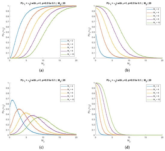
Figure 1.
In each diagram predicted results are plotted as solid curves and empirical probabilities from 10,000 simulations are computed and plotted as dots. (a) with , ; (b) with , ; (c) with , ; (d) with , . Each diagram shows plots for several values.
Note that, in the first three diagrams, and , so we have
and, by the independence of and s and since s are i.i.d.,
so both components grow at the same rate in this example, and it provides a good opportunity to analyse the effect of the thresholds in isolation.
As increases, the probability that is crossed first increases in Figure 1a and the probability that is crossed first decreases in Figure 1b, which is an intuitive result. Further, the probability that they are crossed simultaneously peaks when in each case in Figure 1c.
In Figure 1d, by increasing , this only increases the average jump in the second component, , which makes crossing more likely to occur more quickly, so the probabilities drop to 0 more quickly than in Figure 1b.
In this subsection, we have applied the result from Section 3 to a problem related to the reliability of networked structures experiencing node failures or attacks that incapacitate geometric batches of nodes, each with exponentially distributed weights. In particular, we have derived the probabilities that node losses enter a critical state before, at the same time, or after the weight loss reaches critical levels given the parameters of the distributions and the thresholds. The formulas are numerically very tractable as the regularised gamma functions can easily be computed to high precision. The formulas are also shown to match simulated results to very high precision in several special cases.
A primary practical benefit of these probabilities is that it indicates where weaknesses lie in the network—with node losses or with weight losses. If node loss is likely to become critical first, one should implement interventions that strengthen this aspect of the network, and vice versa with weight loss. Pairing these results on the order of threshold crossings and marginal probabilistic results about the first crossing times and the extent of losses of each type upon crossings in [38,39,45] provides a suitably full understanding of the dynamics of such a process as it approaches and enters a critical state.
While the geometric and exponential distributional assumptions on node and weight losses may seem limiting, they were only needed to invert the operators. The underlying results hold with much more minimal assumptions on the losses, and the same inversion process generally works for many other well-known distributions and empirical distributions derived from data, several of which are shown in [39,45].
Next, we demonstrate that Theorem 1 leads to analytically, or at least numerically, tractable results for two other models, both with explicit inversion and with a numerical approximation.
4.2. 2D Exponential Model
Suppose that each is a vector of two independent exponential random variables with parameters and and Laplace–Stieltjes transforms and ; then,
Here, , so we have , so there are only three possible weak orderings of threshold crossings, which we derive in the following corollary to Theorem 1.
Corollary 3.
If is a vector of independent exponential random variables with parameters and for each n,
and , where is the modified Bessel function of the first kind.
Proof.
Theorem 1 implies
If we assume that ’s and ’s are exponential with parameters and ,
Then, the innermost inverse Laplace transform is
Therefore, noting
we have
can be derived by simply interchanging the parameters and and interchanging the thresholds and , while trivially, which completes the probabilities for each weak ordering in . □
The expressions (58) and (59) are numerically very tractable since the modified Bessel function of the first kind can be computed to high numerical precision efficiently. The practicality of the results is demonstrated by computing them numerically and comparing them to simulated probabilities in Figure 2.
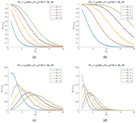
Figure 2.
In the diagrams, predicted results from Corollary 3 are plotted as solid curves and empirical probabilities from 10,000 simulations are computed and plotted as dots. (a) with ; (b) with ; (c) with ; (d) with . Each diagram shows plots for several values.
4.3. 3D Exponential Model
Suppose that each is a vector of three independent exponential random variables with parameters , , and and Laplace–Stieltjes transforms , , and . Then,
We will apply Theorem 1 to derive several results giving the probability of , , , and , which trivially generate probabilities of every other weak ordering of threshold crossings by interchanging the roles of the , , and terms and interchanging the operators.
Corollary 4.
If is a vector of independent exponential random variables with parameters , , and for each n,
Proof.
By Theorem 1,
where
Let , and then
Let , and then
Then, we can find the probability by applying the final inverse Laplace transform with respect to , i.e., equals
□
As we will show later, this can be approximated to high precision by numerical integration and numerical Laplace inversion.
The probability of any other weak ordering in the form for some permutation p follows trivially by interchanging the roles of the variables.
Corollary 5.
If is a vector of independent exponential random variables with parameters , , and for each n,
Proof.
By Theorem 1,
where
Let , and then
Let , and then
Then, we can find the probability by applying the final inverse Laplace transform with respect to , so
□
Note that this formula trivially generates the probabilities of and by interchanging the appropriate variables.
Corollary 6.
If is a vector of independent exponential random variables with parameters , , and for each n,
Proof.
By Theorem 1,
where
Let , and then
Let , and then
Then, we can find the probability by applying the final inverse Laplace transform with respect to , so
□
Note that this formula trivially generates the probabilities of and by interchanging the appropriate variables.
Corollary 7.
If is a vector of independent exponential random variables with parameters , , and for each n,
Proof.
By Theorem 1, is the result of applying to
so
where
Let , and then
Let , and then
Lastly, the probability is the last inverse Laplace transform with respect to applied to the formula above. □
Computational and Simulated Results
The corollaries above establish that these formulas hold, but what may not be clear is that the formulas are actually quite numerically tractable, even with modest computational resources, as we will demonstrate.
The inverse Laplace transforms above that could not be calculated explicitly were computed using a MATLAB implementation by McClure [43] of the fixed Talbot algorithm developed by Talbot [42], which uses trapezoidal integration along a deformed contour in the Bromwich inversion integral. The approach is not exactly the same as Talbot’s original algorithm, but uses some ideas from the framework of Abate and Whitt [44], and the code is optimised for MATLAB by McClure. A similar numerical approach was used to find probabilities in the context of oscillating random walks by Dshalalow and Liew [15], but, in contrast, the results in this subsection are more extensive and involve comparisons with empirical results from simulations.
Note that, for each set of parameters, the probabilities of the weak orderings are listed in the third column of Table 1, ordered in the following way:

Table 1.
In each row of the table, we set some parameter values and compute the probability for each weak ordering by Corollary 4 (line 1), Corollary 5 (line 2), Corollary 6 (line 3), and Corollary 7 (line 4), rounded to the nearest thousandth. Lastly, we have the sum of absolute errors for all thirteen probabilities and the maximum individual error compared to empirical probabilities of each weak ordering computed from 1,000,000 simulated paths of the process.
The testing above and results in the Table 1 reveal some intuitive results about the probabilities:
- In parameter sets (1)–(4), we have and , so, in each line of the results for each set, the probabilities are the same since there is symmetry between the dimensions such that they are indistinguishable.
- In parameter sets (1)–(4), the s are 1 and the s are equal but increasing. Since the process must travel further to cross thresholds while the distribution of the jumps is fixed, simultaneously crossing multiple thresholds (lines 2–4) becomes less probable.
- Comparing parameter sets (5)–(7) to (1) reveals that increasing a single decreases the mean jump length in coordinate j so that is likely to be crossed later than others. Here, we increase , and the probabilities of , , and , precisely where is crossed last, grow.
- Comparing parameter sets (8)–(10) to (1) reveals that increasing a single has a similar effect as increasing a single :
- −
- Parameter set (8) doubles (doubling the distance to cross ) and parameter set (6) halves (doubling mean jump length in dimension 1), which have the precisely same impact on the probabilities.
- −
- Parameter sets (7) and (9) exhibit an analogous relationship.
While the testing above reveals some details of the relationship between the parameters and probabilities, its scope is constrained by our choice of only 10 sets of parameters, so further testing took a large sample random parameters, computed the predicted and empirical probabilities, and compared them. In particular, we sampled sets of the six parameters, with chosen from a uniform distribution on population and from a uniform distribution on , and compared the results to empirical results.
Note the boundaries of the intervals are somewhat arbitrarily selected within a region where an existing MATLAB implementation of the fixed Talbot algorithm for numerical inverse Laplace transforms generally converges properly, with a few exceptions (2% of the sampled parameters).
A random sample of 500 sets of parameters from the distributions mentioned above was taken, the process was simulated 100,000 times for each set, and the predicted and empirical probabilities were compared. In 10 samples, the numerical inverse Laplace transform failed due to rounding or overflow errors, but in the remaining 490 cases, predictions again showed good matching with empirical results. In the worst case, the sum of errors between empirical and predicted reached 0.023, with a maximum individual error of 0.012. This is quite accurate, but even this is an outlier—in the other 489 cases, the maximum sum of errors is 0.012, with maximum individual error 0.004.
4.4. Further Applications of
The tractable formula for found in Theorem 1 has further applications in insurance, finance, reliability theory, and more advanced stochastic network models. Herein, we discuss two of these areas as a motivation for further study and adoption of the present modeling approach in diverse disciplines. Lastly, we will consider the versatility of the result in a more mathematical sense.
4.4.1. Applications to Insurance
Insurance companies receive a random number of claims from their customers per month, each with a random, nonnegative cost to the company. Assuming that the company has a budget of agents to adjudicate claims and a planned budget for costs, then it will be of interest which budget will be exhausted first. If the agent budget is highly likely to exhausted first, the company may optimise its resources by shifting some of the funds pre-allocated for paying the claims to hiring more agents. If the claims budget is highly likely to be exhausted first, the company may optimise resources by hiring fewer agents.
If the distributions of claims per unit time and cost per claim are time-independent, this example is essentially equivalent to the stochastic network application from Section 4.1 above, with equal to the number of claims received in month j and the sum of the costs of those claims in month j. However, the distributions of claims per month or cost per claim need not be geometric and exponential, respectively.
While this two-dimensional problem does not exceed the capabilities inherent in the methods of prior works on stochastic networks [38], the problem becomes far more complex and higher-dimensional if we consider claims budgets in a localised sense. For example, if agents or funding for claims need to be assigned to certain cities, there may be city-specific budgets, and the probabilities of certain orders of these budgets being exhausted can be used to study the effects of allocating agents to different cities. Likewise, a company with diverse offerings may need to assign specialist agents to claims on home, auto, health, or life insurance.
4.4.2. Reliability Theory
The model can also be used to analyse a complex system made up of numerous deteriorating parts. For example, some approaches [48] model the deterioration of a part as a renewal-reward process where the jumps consist of a sum of a continuous deterioration (e.g., linear) plus a random number of “shocks” that introduce damage of random magnitudes approaching a threshold of irrecoverable failure.
The present work can allow such models to be extended to complex systems and determine the most likely order(s) of failures of multiple parts critical to the operation of the system. Such systems frequently require upkeep and repairs to different types of parts, so understanding the most vulnerable parts given these likely orders can allow administrators to design maintenance programs to ensure consistent, reliable operation of the system.
4.4.3. Versatility of Theorem 1
A point that may be missed in the focus on finding the probability of a fixed weak ordering of threshold crossings, , is that they trivially can build probabilities of weak orderings of subsets of thresholds.
For example, in a three-dimensional model, we may have a weak ordering of two of the threshold crossings. Since any weak ordering of a subset can be represented as a sum of some distinct weak orderings, in this case,
The probability of V is, then, the sum of the probabilities of the weak orderings on the right side, all of which are given by Theorem 1 as follows:
As such, while Theorem 1 focuses on probabilities of weak orderings of all the threshold crossings, these results can be summed to obtain the probability of a weak ordering of a subset of threshold crossings. Moreover, in this case, the sum actually simplifies the expression tremendously.
In addition, identifying the likely first threshold crossing can be important. In the stochastic network problem, this identifies the most vulnerable aspect of the network. In insurance, it locates the first budget likely to be exhausted. In reliability problems, it can find the first part that will likely need maintenance. In each case, identifying the likely vulnerabilities can help to determine appropriate strategies to avoid such problems.
Mathematically, this means that we find for each , i.e., the probability that the kth threshold will be crossed first. Clearly, any such probability will be the sum of all probabilities of weak orderings of threshold crossings where comes first—precisely what Theorem 1 expresses.
5. Significance and Future Work
The work above can reasonably be expected to extend in several directions, some of which are the subject of current and future projects.
Closed-form expressions for have been derived by brute force for dimensions and in a similar setting by Dshalalow [12], as well as in the context of a continuous-time marked random walk by Dshalalow and Liew [30]. Although the setting is different in the latter case, the approach and result are quite similar. Their approach was to derive separately for each and add them together, but the size of grows very quickly with d; in fact, it grows at a super-factorial rate since the set of total orderings of the threshold crossings grows factorially, but is only a subset of . The number of weak orderings follows the pattern of the Fubini numbers (also called the ordered Bell numbers), 3, 13, 75, 541, 4683, 47,293, …, so the brute force approach quickly becomes impractical to carry out by hand. The author did some prior work on an algorithmic solution [45], but even listing all the elements of poses computational problems for current consumer-grade computers at dimension 7 or 8. More extensive computational power would not be able to handle much beyond this on a practical time scale given the super-factorial rate of growth.
However, the result of Theorem 1 provides a path to representing an arbitrary in finite dimension d in a manageable formula. An ongoing project seeks to either confirm a conjecture from Dshalalow and Liew [30] or correct it by deriving a closed-form expression for
through a recursive approach exploiting patterns in the expressions.
Further, it is possible to move beyond discrete-time stochastic processes. For example, some prior studies [14,38,39] have considered (continuous-time) marked random walks with multidimensional jump times forming a renewal process for small d with each random vector actually being the d-dimensional jump , which are i.i.d. in this scenario. This work can be adapted to find a joint LST for the position and time of the exit of such a process, , in terms of a joint LST of the jump vector and time between jumps, .
Funding
This research received no external funding.
Data Availability Statement
Not applicable.
Conflicts of Interest
The author declares no conflict of interest.
References
- Wald, A. On cumulative sums of random variables. Ann. Math. Stat. 1944, 15, 283–296. [Google Scholar] [CrossRef]
- Andersen, E.S. On sums of symmetrically dependent random variables. Scand. Actuar. J. 1953, 1953, 123–138. [Google Scholar] [CrossRef]
- Takács, L. On a problem of fluctuations of sums of independent random variables. J. Appl. Probab. 1975, 12, 29–37. [Google Scholar] [CrossRef]
- Takács, L. On fluctuations of sums of random variables. In Sudies in Probability and Ergodic Theory. Advances in Mathematics. Supplementary Studies; Rota, G.C., Ed.; Academic Press: New York, NY, USA, 1978; Volume 2, pp. 45–93. [Google Scholar]
- Erdös, P.; Kac, M. On the number of positive sums of independent random variables. Bull. Am. Math. Soc. 1947, 53, 1011–1021. [Google Scholar] [CrossRef]
- Feller, W. On the fluctuations of sums of independent random variables. Proc. Natl. Acad. Sci. USA 1969, 63, 637–639. [Google Scholar] [CrossRef] [PubMed]
- Chung, K.L. On the maximum partial sum of independent random variables. Proc. Natl. Acad. Sci. USA 1947, 33, 132–136. [Google Scholar] [CrossRef] [PubMed]
- Teicher, H. On random sums of random vectors. Ann. Math. Stat. 1965, 36, 1450–1458. [Google Scholar] [CrossRef]
- Iglehart, D.L. Weak Convergence of Probability Measures on Product Spaces with Applications to Sums of Random Vectors; Technical Report 109; Department of Operations Research, Stanford University: Stanford, CA, USA, 1968. [Google Scholar]
- Osipov, L. On large deviations for sums of random vectors in Rk. J. Multivar. Anal. 1981, 11, 115–126. [Google Scholar] [CrossRef]
- Borovkov, A.; Mogulskii, A. Chebyshev-type exponential inequalities for sums of random vectors and for trajectories of random walks. Theory Probab. Its Appl. 2012, 56, 21–43. [Google Scholar] [CrossRef]
- Dshalalow, J.H. On the level crossing of multi-dimensional delayed renewal processes. J. Appl. Math. Stoch. Anal. 1997, 10, 355–361. [Google Scholar] [CrossRef]
- Dshalalow, J.H. Time dependent analysis of multivariate marked renewal processes. J. Appl. Probab. 2001, 38, 707–721. [Google Scholar] [CrossRef]
- Dshalalow, J.H.; Liew, A. On exit times of a multivariate random walk and its embedding in a quasi Poisson process. Stoch. Anal. Appl. 2006, 24, 451–474. [Google Scholar] [CrossRef]
- Dshalalow, J.H.; Liew, A. Level crossings of an oscillating marked random walk. Comput. Math. Appl. 2006, 52, 917–932. [Google Scholar] [CrossRef][Green Version]
- Novikov, A.; Melchers, R.E.; Shinjikashvili, E.; Kordzakhhia, N. First pasage time of filtered Poisson process with exponential shape function. Probabilistic Eng. Mech. 2005, 20, 57–65. [Google Scholar] [CrossRef]
- Jacobsen, M. The time to ruin for a class of Markov additive risk processes with two-sided jumps. Adv. Appl. Probab. 2005, 37, 963–992. [Google Scholar] [CrossRef]
- Crescenzo, A.D.; Martinucci, B. On a first-passage-time problem for the compound power-law process. Stoch. Model. 2009, 25, 420–435. [Google Scholar] [CrossRef]
- Bo, L.; Lefebre, M. Mean first passage times of two-dimensional processes with jumps. Stat. Prob. Lett. 2011, 81, 1183–1189. [Google Scholar] [CrossRef]
- Coutin, L.; Dorobantu, D. First passage time law for some Lévy processes with compound Poisson: Existence of a density. Bernoulli 2011, 17, 1127–1135. [Google Scholar] [CrossRef]
- Kadankov, V.F.; Kadankova, T.V. On the distribution of the first exit time from an interval and the value of the overjump across a boundary for processes with independent increments and random walks. Random Oper. Stoch. Equ. 2005, 13, 219–244. [Google Scholar] [CrossRef]
- Kadankova, T.V. Exit, passage, and crossing time and overshoots for a Poisson compound process with an exponential component. Theory Probab. Math. Stat. 2007, 75, 23–29. [Google Scholar] [CrossRef][Green Version]
- Aurzada, F.; Iksanov, A.; Meiners, M. Exponential moments of first passage time and related quantities for Lévy processes. Math. Nachrichten 2015, 288, 1921–1938. [Google Scholar] [CrossRef]
- Bernyk, V.; Dalang, R.C.; Peskir, G. The law of the supremum of stable Lévy processes with no negative jumps. Ann. Probab. 2008, 36, 1777–1789. [Google Scholar] [CrossRef][Green Version]
- White, R.T.; Dshalalow, J.H. Characterizations of random walks on random lattices and their ramifications. Stoch. Anal. Appl. 2019, 38, 307–342. [Google Scholar] [CrossRef]
- Chaumont, L.; Marolleau, M. Fluctuation theory for spectrally positive additive Lévy fields. arXiv 2019, arXiv:1912.10474. [Google Scholar] [CrossRef]
- Borovkov, K.A.; Dickson, D.C.M. On the ruin time distribution for a Sparre Andersen process with exponential claim sizes. Insur. Math. Econ. 2008, 42, 1104–1108. [Google Scholar] [CrossRef]
- Yin, C.; Shen, Y.; Wen, Y. Exit problems for jump processes with applications to dividend problems. J. Comput. Appl. Math. 2013, 245, 30–52. [Google Scholar] [CrossRef]
- Yin, C.; Wen, Y.; Zong, Z.; Shen, Y. The first passage problem for mixed-exponential jump processes with applications in insurance and finance. Abstr. Appl. Anal. 2014, 2014, 571724. [Google Scholar] [CrossRef]
- Dshalalow, J.; Liew, A. On fluctuations of a multivariate random walk with some applications to stock options trading and hedging. Math. Comput. Model. 2006, 44, 931–944. [Google Scholar] [CrossRef]
- Kyprianou, A.E.; Pistorius, M.R. Perpetual options and Canadization through fluctuation theory. Ann. Appl. Probab. 2003, 13, 1077–1098. [Google Scholar] [CrossRef]
- Mellander, E.; Vredin, A.; Warne, A. Stochastic trends and economic fluctuations in a small open economy. J. Appl. Econom. 1992, 7, 369–394. [Google Scholar] [CrossRef]
- Dshalalow, J.H. Random walk analysis in antagonistic stochastic games. Stoch. Anal. Appl. 2008, 26, 738–783. [Google Scholar] [CrossRef]
- Dshalalow, J.H.; Iwezulu, K.; White, R.T. Discrete operational calculus in delayed stochastic games. Neural Parallel Sci. Comput. 2016, 24, 55–64. [Google Scholar]
- Takács, L. Introduction to the Theory of Queues; Oxford University: Oxford, UK, 1962. [Google Scholar]
- Dshalalow, J.H.; Merie, A.; White, R.T. Fluctuation analysis in parallel queues with hysteretic control. Methodol. Comput. Appl. Probab. 2019, 22, 295–327. [Google Scholar] [CrossRef]
- Ali, E.; AlObaidi, A. On first excess level analysis of hysteretic bilevel control queue with multiple vacations. Int. J. Nonlinear Anal. Appl. 2021, 12, 2131–2144. [Google Scholar] [CrossRef]
- Dshalalow, J.H.; White, R.T. On reliability of stochastic networks. Neural Parallel Sci. Comput. 2013, 21, 141–160. [Google Scholar]
- Dshalalow, J.H.; White, R.T. On strategic defense in stochastic networks. Stoch. Anal. Appl. 2014, 32, 365–396. [Google Scholar] [CrossRef]
- Abolnikov, L.; Dshalalow, J.H. A first passage problem and its applications to the analysis of a class of stochastic models. Int. J. Stoch. Anal. 1992, 5, 83–97. [Google Scholar] [CrossRef]
- Polyanin, A.; Manzhirov, A. Handbook of Integral Equations; Chapman and Hall/CRC: Boca Raton, FL, USA, 2008. [Google Scholar] [CrossRef]
- Talbot, A. The accurate numerical inversion of Laplace transforms. IMA J. Appl. Math. 1979, 23, 97–120. [Google Scholar] [CrossRef]
- McClure, T. Numerical Inverse Laplace Transform. MATLAB Central File Exchange. 2022. Available online: https://www.mathworks.com/matlabcentral/fileexchange/39035-numerical-inverse-laplace-transform (accessed on 5 June 2022).
- Abate, J.; Whitt, W. A unified framework for numerically inverting Laplace transforms. INFORMS J. Comput. 2006, 18, 408–421. [Google Scholar] [CrossRef]
- White, R.T. Random Walks on Random Lattices and Their Applications. Ph.D. Thesis, Florida Institute of Technology, Melbourne, FL, USA, 2015. [Google Scholar]
- Al-Matar, N.; Dshalalow, J.H. Time sensitive functionals in a queue with sequential maintenance. Stoch. Model. 2011, 27, 687–704. [Google Scholar] [CrossRef]
- Dshalalow, J.H.; Merie, A. Fluctuation analysis in queues with several operational modes and priority customers. TOP 2018, 26, 309–333. [Google Scholar] [CrossRef]
- Dshalalow, J.H.; White, R.T. Random walk analysis in a reliability system under constant degradation and random shocks. Axioms 2021, 10, 199. [Google Scholar] [CrossRef]
Publisher’s Note: MDPI stays neutral with regard to jurisdictional claims in published maps and institutional affiliations. |
© 2022 by the author. Licensee MDPI, Basel, Switzerland. This article is an open access article distributed under the terms and conditions of the Creative Commons Attribution (CC BY) license (https://creativecommons.org/licenses/by/4.0/).