1. Introduction
In numerous biological applications related to the proliferation of microorganisms, such as bacteria, viruses, and even cancer cells, at some point of their division, they start mutating. New mutants are typically stronger and more virulent. In most common situations, bacteria divide in two forming a deterministic branching process. If a colony starts from a single organism, in the
nth generation, its population size is
(unless some progenies perish). Suppose at some point that one of its offspring mutates, say, with probability
(which is typically small). Then, a new mutant divides like a nonmutant and it engenders a deterministic branching process. As the rate of reverse mutation on the same phenotype, called
revertant, is extremely small [
1,
2], we do not consider this option in our paper. The mutation probability
is called the
mutation rate.
1.1. Our Approach Compared to Other Methods
The mutation rate is a common target in biomedical research and its applications. Ever since the seminal paper by Luria and Delbrück [
3] in 1943, numerous works on determination of mutation rate have emerged (cf., [
4,
5,
6,
7,
8,
9,
10,
11,
12,
13,
14]). They all have dealt with various estimates for
.
The deterministic branching process (a rooted tree) contained a branching subprocess (random subtree) of non mutants that turned out to be a Galton–Watson process, although the target process was that of new mutants. The new mutants and pre-existing mutants form non-Markov processes.
Why do we deem the branching processes approach more rigorous? In Luria and Delbrück [
3], the authors assumed that the number of mutations
that occur in interval
equals
, where
is the total number of bacteria at time
t. This assumption is inaccurate, because to determine the mutation rate
, they had to exclude from
the number of pre-existing mutants, even if this number is small. We actually prove that even if the mutation rate
is small, the number of pre-existing mutants can converge to infinity and thus cannot be neglected. Moreover,
would be better off to equal some
, where
is the number of nonmutants at time
t, which doubles in interval
unless
is too small. Stewart [
15] also states that the Luria and Delbrück method is inaccurate.
Furthermore, if that would not be the case and
would be approximately equal to the number of nonmutants at time
t, then the Luria and Delbrück method is still problematic. Here is why: suppose
is the number of nonmutants in generation
n and suppose that each nonmutant can turn to a mutant with equal probability
. Thus, each nonmutant is a Bernoulli r.v. with parameter
. The number of newly born mutants
in generation
n is thus binomial with parameters
, that is,
. Because
is large and
is small, the number
is approximately Poisson, with parameter
, which carries unknown
and
. The probability that there is no mutant at generation
n would have been
, which the authors claimed could be determined experimentally and is fairly simple. However, there is still a problem of finding
, which is not equal to the total number cells
, nor does it equal the number of all mutants
at generation
n. This is the reason why we think this method is unpredictably inaccurate (although Zheng in [
16,
17] claims that the Luria/Delbrück method is the best). Precisely,
(≠
as the authors allude), provided that the latter is consistent in some sense and that
n is sufficiently large. None of these requirements has ever been met in their work, nor in the work of their followers. This problem was also pointed out by Stewart [
15].
Another problem in the statistical evaluation of the popular -method is that in order to maintain a “nonmutant” plate (which is required to reasonably estimate ), it applies to counts rendered at early times or for cultures with extremely low mutation rates to warrant at least one plate with no mutants. However, this carries an adverse effect on statistical significance.
In various other alternatives, many formulas contain the ratio as a major component in their estimators (rather ) which has a similar shortcoming and it cannot be salvaged by logarithmic or other multipliers often occurring in the literature. We noticed that no work offers a general formula for the determination of (whether practical or not). All heuristic methods may work in some special cases, but none are claimed to be general. In the literature on mutation rates, we see that some methods claimed to be efficient when following certain heuristic instructions imposed on (which was to be determined) and the mean number of mutants. It is not clear how the results obtained for were validated. We compared several tables of the results produced from different methods and they all vary.
In Niccum et al. [
18], we offered the first rigorous method of determining
by a pointwise rapidly convergent sequence
of estimators. At first, the original formula for
we operated on looked impractical because it contained newly formed mutants that are difficult to tell from pre-existing mutants, but it was modified by replacing it with an identical formula requiring just the knowledge of the mutants in any two consecutive generations that turned out to be practical in real labs. That “it was still difficult to observe” as stated in Zheng [
17] was not the situation with a series of our lab experiments [
18] performed by us and our students (who coauthored the paper) and beyond. It also needs to be noted that the proposed estimator had a rapid speed of convergence that has been validated in numerous subsequent simulations rendered by our students in senior undergraduate and graduate projects with no single exception.
1.2. Synchronized Cultures
In our original mathematical model [
18], we assumed that bacteria replicate synchronously. We retain this mathematical assumption in the present work as well. As explained in [
18], the real count in the lab is a little different. This method has been rendered for decades and the count of mutants (that is compatible with our theoretical assumption) agrees with quite a few experiments made by different researchers, which obviously renders coincidences (and thus inaccuracies) probabilistically impossible.
Yet for the skeptics of our mathematical methodology, we would like to mention the common practice of synchronization of bacterial cultures known in the biological literature. First, a synchronized culture is a culture that contains cells in the same growth stage when they replicate, as opposed to asynchronous growth when the replication cycles are random. Most known cell divisions in a population are asynchronous. It is an observed, although unproven, assumption that random deviations of the cycle lengths are symmetric around the mean time of division. However, that needs to be rigorously validated. If this holds true, it is easy to deduce that a mere observations of a bacterial culture would give a pretty accurate identification of an underlying generation.
Alternatively, there are widely used synchronization approaches from 1957 (cf. Campbell [
19]) and earlier and these continue to be described to the present time (cf. Chang et al. [
20] of 2019). A popular technique, known as Helmstetter–Cummings [
21,
22] of 1968 and 2015 deals with an unsynchronized culture filtered through cellulose nitrate membrane filter. There are numerous other synchronization techniques by Anderson and Pettijohn [
23], Kepes and Kepes [
24,
25], Kubitcheck [
26], Ling and Chang [
27], Noack, Klöden, and Bley [
28], Shehata and Marr [
29], and Wallden et al. [
30], to name a few. A rigorous description of all those methods lies outside the scope of this paper.
Note that experimentally cells may not remain synchronized during growth complicating analysis. As mentioned above, it would be interesting to conduct lab experiments and learn about the statistical impact of unsynchronized replication. It seems that even if we assume the replication to be synchronous while in facts it is not, the deviations will be symmetric and not large, and as the result, the incorrect assumption will not corrupt the counts, because so far, the observed numbers were not conflicting with our experiments, and they agreed with experiments conducted in other labs. This conjecture is by no means intended to replace a rigorous investigation, which we plan to render.
1.3. Mutation or No Mutation?
There are many anecdotal stories about antibiotics causing antibiotic resistance and breeding new forms of virulent bacteria, in quite a few cases offering little to no remedy. One such notorious form is called MRSA, which stands for methicillin-resistant Staphylococcus aureus (S. aureus), a type of bacteria that has become resistant to potent antibiotics used to treat ordinary staph infections. It thus means that it is tougher to treat compared to other strains of Staphylococcus.
MRSA most commonly causes skin infections and can sometimes trigger pneumonia and other conditions. The symptoms largely depend on which part of the body is affected. Untreated, MRSA can become severe, leading to sepsis. MRSA infections are usually seen in individuals who were previously or currently in hospitals or other health care facilities such as dialysis centers or nursing homes. Many professionals are alarmed by the spread of MRSA as due to its resistance to many types of drugs; it is becoming known as a “super bug”.
On the other hand, there is a general consensus that while bacteria mutate, this process is neither impacted nor exacerbated by the use of antibiotics or other chemical agents. They claim that mutations occur periodically without any external force. However, that natural selection allows these to thrive over other bugs that do not have resistance. (It must be noted that antibiotics are natural products of other organisms that also try to keep bacteria away.)
Before we elaborate it, we wonder what a mutation is referred to in cellular/molecular biology. A mutation is formally defined as an alteration to the gene sequence of an organism. A “natural mutation” occurs spontaneously and can happen during bacterial DNA replication where enzymes choose a wrong base to pair with the original DNA, or due to the environmental UV light, modifying the structure of the original DNA strand that allows it to pair with bases that are not normally compatible.
While the entire bacterial genome is susceptible to mutation, certain mutations are more easily detected than others because of selection. An example is the
trpE gene in the
Escherichia coli (
E. coli) WP2 strain [
31]. This high mutation region allows researchers to detect mutation on the strain using the so-called
reverse mutation assay, in which the bacteria are grown in an amino-acid-deficient culture to test if the mutation occurred (
) or not (
) [
32].
The natural mutation rate for
E. coli in a rich medium mutation rate is
per genome per generation [
33]. The mutation rate of
methicillin-resistant Staphylococcus aureus (
S. aureus)—MRSA strain is similar to the reported mutation rate of wild-type
E. coli [
34]. The elevated mutation rate is suspected to cause the increased rate of bacteria vancomycin-resistant genes, especially for the vancomycin-intermediate-resistant
S. aureus strains—VRSA [
35].
1.4. Other Means of Genetic Change
Other means of genetic change exist, in addition to classical spontaneous or genotoxicant-induced mutation, and, in some cases, these resulting genetic changes may also be covered by our model in as much as they may represent stochastic events. While the mechanisms responsible for these changes are well understood and these processes are not considered as classical mutations, they do result in genetic change in the affected organism. In some cases, the probabilities of these events are rare and, as such, the resulting genetic change may be described by probabilistic models. For the purposes of a more comprehensive discussion of other modes genetic changes, these alternative modes of change will be briefly described.
Transformation. Transformation is a process in which a bacteria takes up exogenous (free) DNA from its surrounding environment. This DNA can come from dead (lysed) bacteria. Transformation can happen artificially (such as a heat shock/electroporation), or naturally. A natural transformation occurs when there is a cooperative expression of multiple genes under specific conditions called competence [
36]. This state is induced by a limited nutrition (usually amino-acid-deficient environment), associated with the stationary phase. For some other bacteria, transformation occurs most efficiently at the end of exponential growth approaching the stationary phase.
Transformation is one process that can lead to
Horizontal Gene Transfer (HGT). There is a hypothesis about the HGT facilitated by the transformation of antibiotic-induced cell-wall-deficient bacteria [
37]. This hypothesis states that before the bacteria die, they generate a cell-wall-deficient form and increase the uptake rate of exogenous DNA, because the DNA from dying bacteria release DNA. They are not doing the uptake as they are dead and could not then restore life to propagate this. Combining with the fact that patients who were treated with diverse antibiotics are more prone to get infected with MRSA makes this hypothesis more credible.
In this process, two bacterial cells attach, and plasmids and free intracellular DNA fragments travel from the donor cell to the target cell. In the target cell, plasmids can begin to replicate, whereas DNA fragments may become incorporated in the target cell’s genome. A study on MRSA conjugation stated that this mechanism could be one of the pathways by which methicillin resistance is transmitted among
S. aureus strains [
38].
Transduction. Another mechanism for bacteria genome variation is called
transduction. When bacteria are infected with a virus (usually a bacteriophage), the virus uses the cell’s materials to produce new viruses and kill the bacteria when it reaches some threshold. During the production of new viruses, some fragments of the original bacteria’s DNA are taken up into the virus’ DNA. When this virus infects other cells, it also introduces the DNA to the new cell. If the infection goes to the latent phase and the fragments contain antibiotic genes, the bacteria become antibiotic-resistant [
39]. Virus latency (or viral latency) is the ability of a pathogenic virus to lie dormant (latent) within a cell, denoted as the lysogenic part of the viral life cycle. If virus becomes latent, it neither reproduces nor kills the host cell.
So, as we see it, there is a variety of genetic alterations to the bacteria that are technically not mutations, but they often produce virulent species. While it is a common conjecture that bacteria do not mutate under chemical agents such as antibiotics, the latter does cause formidable DNA changes turning some strains to dangerous forms that can be even life-threatening. Most of these transformations are detectable and they can be observed and analyzed mathematically to determine the odds of their changes whether or not we call them mutations. Therefore, it stands to reason to consider those phenomena and place them in the same category as mutations and apply the same mathematical tools to establish rigorous estimators of their genetic transformations. It is also possible that an epigenetic change can occur that may be detectable by selection.
1.5. The Results
In the present paper, we show that the estimator proposed in [
18] is not only almost surely pointwise consistent but also consistent in the
-norm giving us yet another mathematical confirmation of the goodness of the proposed estimator. We also prove the convergence with respect to other probability measures. We further assume that a microorganism can mutate in one of the two types, which in particular, can model the spread of virulent antibiotics-resistant bacteria (referred to in the media as “superbugs”) that evolve under attacks by chemical agents so that they either die or mutate to survive the attacks. Consequently, mutated or altered bacteria’s variants that survive are referred to as
type 1 mutants and other mutants are called
type 2 mutants. We also propose estimators for either type of mutants. These estimators turn out to be unbiased and consistent in every common sense, that is, almost surely pointwise and in the
-norm. (Some other forms of consistency are discussed throughout the forthcoming sections.)
We note that while death of bacteria is present in most bacterial cultures, it is rarely used in mathematical modeling. We address this matter in the present article and even generalize our model allowing replicated offspring to turn to one of the two mutant types with probabilities p and , respectively. It makes sense to call such division symmetric when . In the event that this represents bacterial death, that, as mentioned, takes place under the use of a chemical agent (such as antibiotic) or bacteriophage attack.
3. A Background on Stochastic Estimators of Mutation Rate
Consider a population of microorganisms, such as bacteria, stemming from a single parent. Assume that the bacteria replicate by the division in exactly two progeny. At generation
n, there are exactly
bacteria in the population forming a deterministic branching process, provided that the bacteria do not die. Suppose that a generation began with a single parent bacterium (at generation zero) and beginning from generation 1, each bacteria, independently of the others, mutates with probability
. The parent bacterium of the generation is thus assumed to be a nonmutant organism. Let
be the total number of nonmutants at generation
n,
be the total number of new mutants at generation
n, and
be the total number of all (preexisting and new) mutants at generation
n. We assume that
(referred to as the
mutation rate) is constant at every generation. To determine
experimentally, we proposed in [
18] the estimator
which turned out to be unbiased and consistent a.s. on the non extinction set
(defined below) such that
, where
. (For various bacteria, such as
E. coli, this probability is extremely close to 1.)
Since the sequence
is monotone decreasing, the notation
in (
2) makes sense and
is referred to as the
nonextinction set. As mentioned above,
.
In light of our next applications, it is more convenient to turn to the confined space
where
If
is a r.v. on the confined space
, then (cf., Dshalalow [
41]), the expected value
(with respect to measure
) is
4. Preliminaries
Let
, be the normalized sequence of the respective nonmutants populations. This sequence is a martingale that almost surely on
converges to a r.v.
(cf. [
42]). Furthermore, Theorem 2 [Section 6, Chapter I] of [
42] reveals the nature of this r.v., also stating that the convergence of
to
is also in the mean square.
Note that Theorem 2 below is borrowed from [
42] originally formulated and proved as Theorem 2. It could be more rigorously crafted under the specification of the confined probability space
introduced in (
3) and (
4). We proceed with those key assumptions throughout the rest of the paper.
Theorem 2 ([
42])
. If then- (i)
.
- (ii)
.
- (iii)
.
From Theorem 2 (), we have that .
Assume that
. Since
with the distribution
and
, respectively, the sequence
converges to
where
is defined on
and valued in
, with the distribution
and
, respectively. Therefore, on the confined probability space,
,
equals
∞-a.s. Hence, the r.v.
on
equals
-a.s., which implies that
Now, because
on
,
on
. Therefore,
Because
is
-integrable, using the Lebesgue dominated convergence theorem (LDCT),
Thus, we proved the following lemma,
Lemma 1. , where and are the integrals on respective spaces and .
Next, recall [
18] that
is the number of new mutants at generation
equal to
Similarly, because
a.s. on
it follows that
on
that implies
By the LDCT and because
Using the same arguments as in the proof of Lemma 1, we easily conclude that
In a nutshell,
Lemma 2. , where and are the integrals on respective spaces and .
6. The Speed of Convergence
In [
18], we validated the pointwise convergence of estimator
to
by simulation and most importantly noticed that the speed of convergence was fast. Considering the replication time of various bacteria (20–40 min), it generally takes not more than 12 to 15 h of lab experiments (or 25 to 30 generations) to attain to a high accuracy approximation of
. We wondered if similar qualities of
apply to the
-convergence (mean square) in some form. The considerations below are carried out in the confined space
.
Then, is 1 if the ith nonmutant mutates and 0 otherwise.
We drop the superscript
n in
, and
assuming that they are iid Bernoulli r.v.’s with parameters
and
, respectively. Then,
and
implying that
Setting (constant), is the sample mean of Bernoullir.v.’s and thus with large, by the CLT (central limit theorem), has a Gaussian distribution with parameters (mean) and (variance). Now, with n being just 10 or larger and small, must be a large number. Thus, with simulation, because is obtained empirically it is a constant and as noticed , good for all . The variance of is small and must approach 0.
Suppose we “observe” bacterial replication on
M plates where each colony starts with a single parent. Denote
the estimator associated with
kth plate,
. For notational brevity, we will use the same symbol
for its estimate (i.e., observed value). Denote by
the sample mean of
M estimators (estimates)
. Thus,
is the unbiased sample variance that is known to be consistent and weakly convergent to
as
. However, we expectthat
rapidly converges to 0 with just reasonable
n and
M. This would be a heuristic feel of the true convergence speed of the variance of
(cf. Equation (
12)).
Example 1. To validate the results above, we will simulate the process for several fixed values of μ and compute the sample estimates of the mean and variance of μ, i.e., and , for generations for different numbers of plates ranging from to . The goals are twofold: (1) to validate the accuracy of the estimators empirically and (2) to experimentally examine the convergence of the estimators for various choices of generations n and plates M. The estimators are more promising for practical use if convergence occurs for relatively small n and M.
To compute estimates, we must simulate M paths of the process for each experiment. For each sample path, we start with nonmutant at the 0th generation and, for each generation , we assume the number of nonmutants is a binomial random variable for a preselected mutation rate . We generated M paths from to . The estimated mutation rate is computed at each generation to as (rewritten as for convenience) and the mean is taken for each experiment with M plates. The sample variance will also computed. Ideally, the estimate will be near and the estimate will approach 0 quickly for relatively small M.
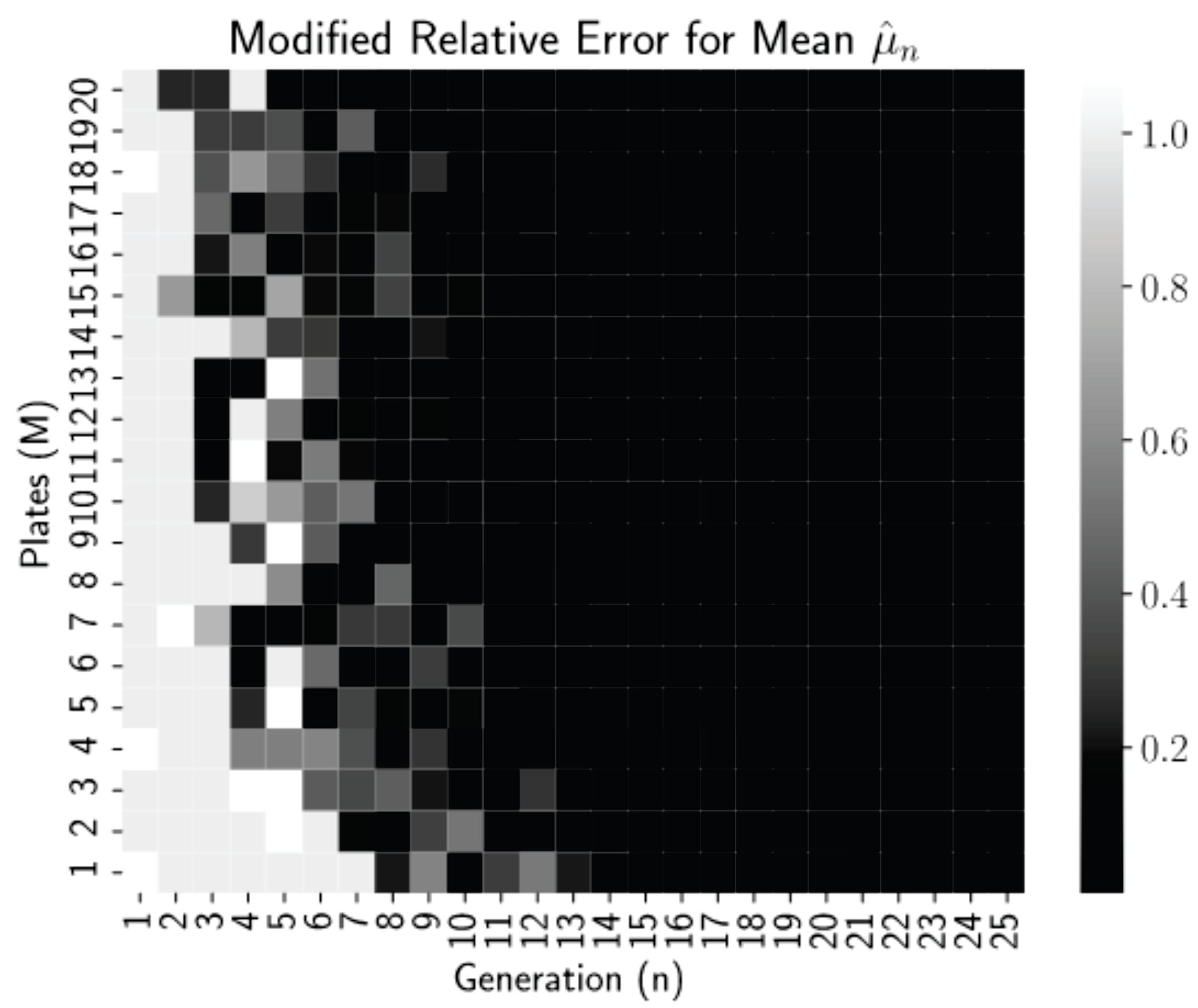
We follow this approach in several examples. In
Figure 1, we let
and simulated the experiment for 25 generations for each selection of plates
(We did not use
as we evaluate sample variance with degree of freedom of 1). There are several intuitive occurrences here.
Since
, the estimate is 0 if there are no new mutants in generation
. As we see in
Figure 1, the estimates are indeed 0 before the first mutant appears in each experiment. An interesting pattern emerges here: for
and
plates, the first mutant appears in generation 1 and 2, respectively; for
plates, the first mutant appears at generation 3; and for
, the first mutant appears at generation 4. The time of the first mutation is inversely related to the number of plates, which makes sense because there are more opportunities for mutations with more plates and, therefore, the estimate is nonzero sooner with more plates.
Second, the estimates behave erratically between the initial escape from 0 until roughly generation 7–8. During the early generations, there are smaller nonmutant populations in the plates, meaning intuitively that the random mutations have larger impacts on the estimates.
As such, variance is higher when the prior generation’s nonmutant population is smaller, and this nonmutant population grows over time in expectation since the mutation rate , so we should expect to high variances in early generations. After 7 or 8 generations, the variance seems to dissipate enough to allow the estimates start to approach the true mutation rate .
Continuing beyond generation 8, estimates in all experiments approach , with the experiments with fewer plates, especially , taking a longer time to converge—again, this is expected as the conditional variance of is inversely proportional to , and a shrinking variance should result in convergence of the unbiased estimator.
Clearly, and unsurprisingly, the estimates have higher quality for larger generation
n and larger number of plates
M, but more interestingly, what does this mean for experimental use of the estimator? First, we define a modified relative error for the estimate
which is the relative error or 0.01, whichever is larger.
Figure 2 is a heatmap of this modified relative error for each pair
n and
M from our simulations.
Thresholding the relative error as
allows us to see clearly in
Figure 2 that relative errors of less than 0.01 occurred for all generations
regardless of the number of plates, but for more plates, near
, these small errors occur reliably earlier, at generations
. Thus, even low numbers of plates can be used if the experiment can continue for more generations. This is a promising finding for biology lab protocol, as growing more than 20–25 dishes per experiment is highly infeasible. After 15–20 generations (starting with 1 starting cells), we have the mean converged.
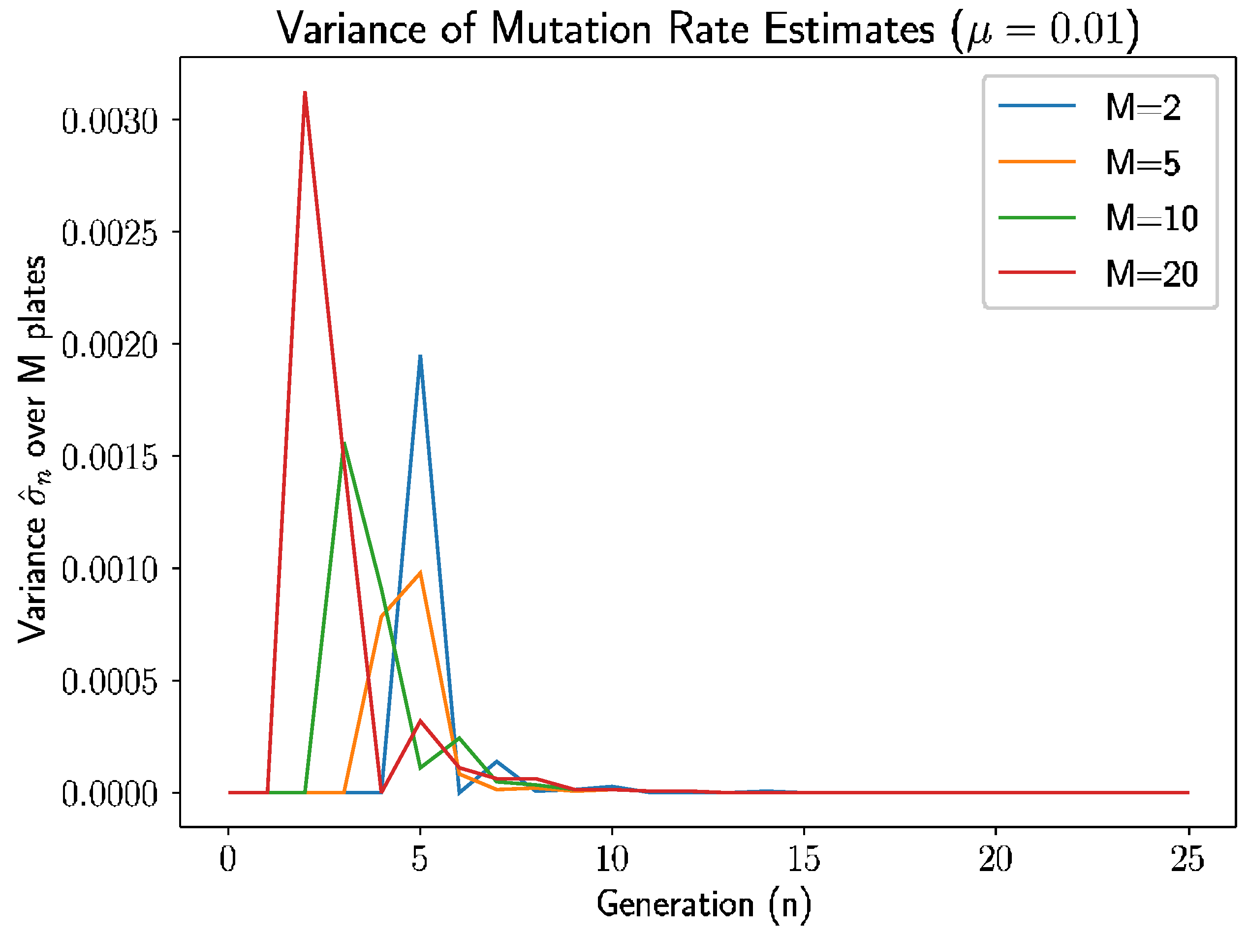
Beyond the behavior of the mean mutation rate themselves, we can consider the estimated variance of the mutation rate,
.
Figure 3 shows the estimated sample variance for several experiments with
and 20 plates.
As we see in
Figure 3, the variance converges to 0 within 10–12 generations regardless of the number of plates, as prior analysis suggested should happen.
7. Estimator
We now assume that once a cell or microbe mutates, it turns into one of the two mutant types, with probabilities p and respectively. The type i mutant then divides in accordance with a deterministic branching process throughout the generations and it does not mutate any further, nor does it alter its type. In particular, we can also interpret mutation types as a continual existence upon mutation (type 1) with probability p or the death (type 2) with probability . Note that our analysis in this section is interchangeably carried out in the original and confined probability spaces and respectively. In all cases, the underlying functionals can be distinguished by the absence or presence of subscript 0.
Denote by
the proportions of type 1 and 2 new mutants at the
nth generation from among the
new mutants, respectively. We will show that the estimator
is unbiased and consistent (and so is
).
Recall that . Denote . Below, we observe an interesting and unexpected result concerning the sequence . Whereas it obviously is not monotone, as the following two assertions show, the sequence of their measures under a weak and natural assumption, is strictly monotone increasing (we recollect that the sequence with respect to nonmutants is monotone nonincreasing) and furthermore, like , converges to .
Theorem 4. The following two assertions are valid.
- (i)
- (ii)
If the sequence is strictly monotone increasing.
Proof. - (i)
Let
. Then, because
given
,
- (ii)
We show that is strictly monotone decreasing.
First off,
is strictly monotone increasing for
. Now since
and
,
Now, we show that
or that
Let
. Consider
, where ⋄ stands for one of the three relations,
. We have
or
The discriminant of the equation
is
Furthermore, after some algebra,
where
(is the extinction probability
) and
. Therefore,
(and ⋄ is <) for all
. In conclusion,
Therefore, if
,
. Next, since
is strictly monotone increasing in
and because
, it follows that
Finally, since
is strictly monotone increasing, by the principle of mathematical induction,
that proves the assertion that
is a strictly monotone decreasing sequence and so is the sequence
. □
Corollary 1. .
Proof. Let
. Then, from the equation
we have
Furthermore, since
is monotone decreasing,
exists and it is unique. Because
is continuous, this limit from (
15) can be found from the equation
From the theory of branching processes, we know (cf. Kimmel and Axelrod [
43]) that the extinction probability
is the smallest positive root of the equation
. In our case,
and the extinction probability
if the mean
which is routinely met when
. The equation
has two roots: 1 and the other one
which is the smallest of two. Consequently,
ends up being equal to the extinction probability. Therefore,
□
Since
, given
,
and therefore,
Consequently, is - and -unbiased, where .
Theorem 5. If , converges to p in the -norm, -norm, and a.s. pointwise. Furthermore, is asymptotically -unbiased.
Proof. - (i)
We start off with
implying
Because
,
is
-integrable. By Lemma 2 (cf. Equation (
7)),
Thus, because
is
-unbiased,
- (ii)
Now we show that
The latter is true due to the following: As per our assumption, every new mutation takes place with a constant probability
. The new mutants form process
. The estimator
of
is consistent in the sense that
a.s. pointwise. If a new mutant is formed from a nonmutant, in our present model, it becomes a type 1 new mutant with a constant probability
p, i.e., a type 1 new mutant emerges from a nonmutant with probability
. We then focus on
and
of nonmutants in generation
n and type 1 new mutants in generation
, respectively. We can then reduce this model to the original one with
being a new mutation rate. Thus, we define the estimator
of
as
, and the latter must converge to
a.s. pointwise [
18].
Consequently, from Theorem 3, converges to in the -norm.
- (iii)
Now, we turn to
defined as
. Dividing the numerator and denominator by
, we get
More specifically, if the numerator converges to pointwise on and the denominator converges pointwise to on such that ,then pointwise on set and clearly . Thus, the convergence of to p is a.s. pointwise on .
Because
for all
’s, by the LDCT and Equation (
18),
- (iv)
Thus by the LDCT,
and
so that
is asymptotically
-unbiased. Consequently,
- (v)
□
Remark 1. - (i)
If the second mutation type of bacteria are dead, the formula is impractical for a lab utility, since the dead cells are not counted. Here is a way out.
First, notice that in this case, (i.e., the same formula as for with only one mutation type). This is exactly because the dead bacteria cannot be counted. Next, we have so that the “deficit” of the count is - (ii)
If the second mutation type are not dead bacteria, then , but However, Equation (19) still applies, whereas Equation (20) can be modified as Obviously, Equation (21) can be modified as follows where superscripts and stand for the first and second type mutants, respectively.
In a nutshell, if type one bacteria die upon mutation, the formula for the estimator of p is simple and it does not require one to distinguish the bacteria types. This is not the case with two surviving types, as per Equation (24).
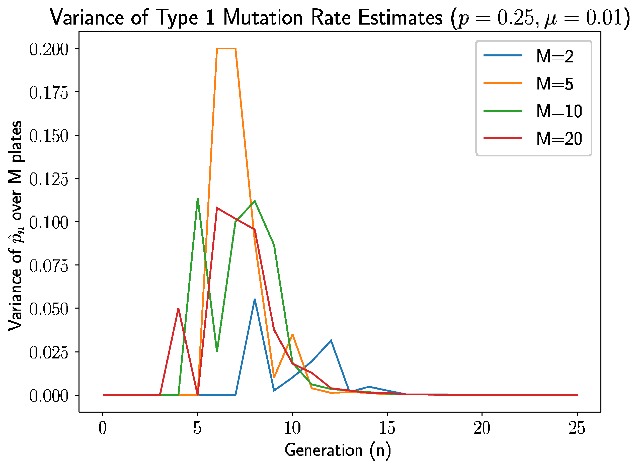
8. Simulation of Estimators for Types 1 and 2
To validate the convergence and its speed, we render simulation analogous to that in
Section 6. After generation of nonmutant paths similar to
Section 6, we evaluate new mutant (all types) at each generation using
. For each new mutant generation, we run a binomial random number generator with distribution
for mutation type 1, assuming type 2 is the rest of the mutation population with distribution
, because
. This new mutant type
i generation is added to the current population of type
i mutant (previous generation mutant doubled):
, with the assumption that
(initially, we have 0 mutants). The algorithm is looped for
n generations and we store the result in a new
matrix with first row being zero row. Type 1 mutation rate is estimated by Equation (
21):
and the output was an
matrix. Mean mutation and variance of the mutation rate were evaluated using the sample variance equation in
Section 6, knowing the convergence is established with Theorem 5.
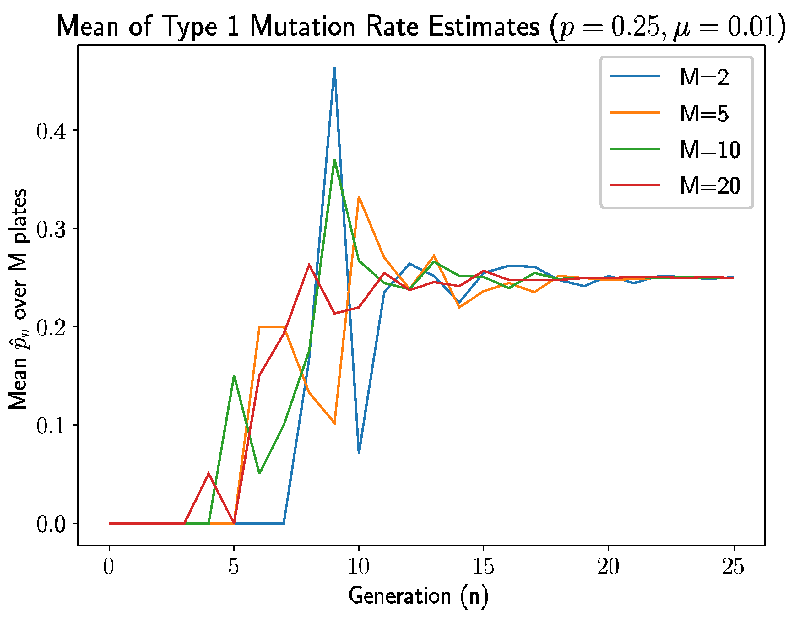
For this simulation, we let the probability that a newly mutated bacterium is of type 1 be
.
Figure 4 is the simulation results—specifically, the mean of the type 1 mutation rate estimate.
Similar to simulation in
Section 6, we see a pattern here: the estimate is 0 if there are no new mutants. In this simulation, first mutation does not occur until generation 3 for
, generation 4 for both
and
, and generation 7 for
. The time of the first type 1 mutant is also inversely related to the number of plates, due to the appearance of type 1 mutation depends on the time of first mutation, which is because of, as discussed previously, more opportunities for mutations to occur with more plates.
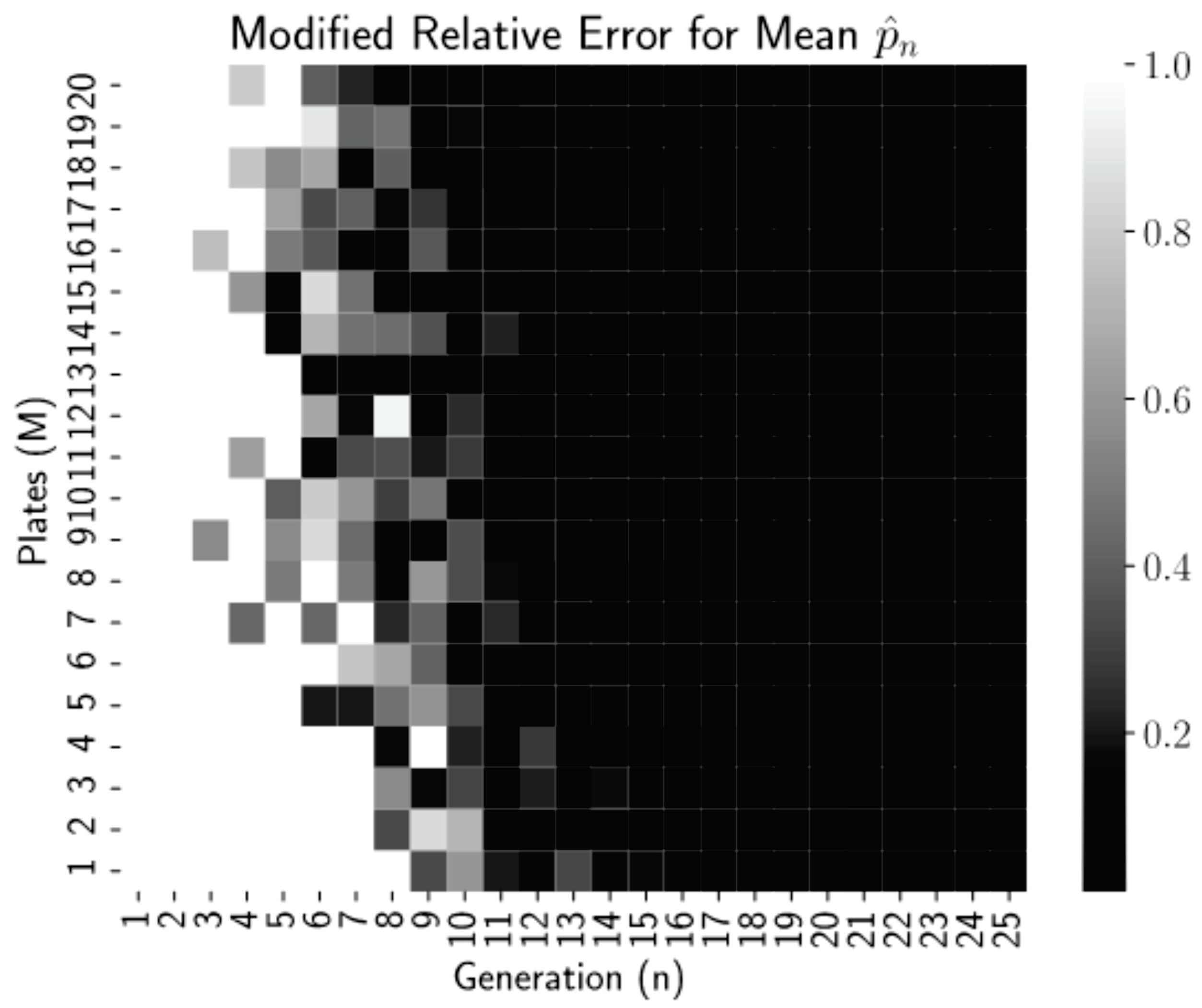
The estimates stabilize after 9–10 generations, which is a couple of generations lag after first mutation occurs, as established above. This can be explained due to the probability of getting type 2 mutation is larger than type 1 and, due to this type 1 mutation, take more generation to appear. The following modified relative error heatmap (
Figure 5) also describes this phenomenon.
Figure 5 shows the similar pattern as
Figure 2: for all generations
, regardless of the number of plates, the relative error is less than 0.01; the more plates there are, the less occurrence of large relative errors in earlier generations. For all number of plates, the threshold for small relative error is
; which is 1 to 2 generation behind the observed threshold from
Figure 2 (
). Similar to
Section 6, this result is a promising finding for biology researchers as the number of dishes is feasibly small to be made in laboratory settings.
As described in
Figure 6, similar to simulation in
Section 6, the estimated variance of
quickly converges to 0 after 13–17 generations (which is also a couple of generations behind the convergence of variance discussed in
Section 6), regardless of the number of plates.
9. Summary
In 2012, Niccum et al. [
18] offered a simple stochastic estimator
of
in a most rigorous fashion proving that it was unbiased and consistent. The latter meant that the sequence
was almost surely pointwise convergent to
on a non extinct set. Best of all, the pointwise convergence proved to be fast, as it was validated by countless simulation runs for various values of
.
In this paper, we studied the stochastic process describing bacterial mutation that begins at some point of their division. In our earlier paper [
18] (by two of the present coauthors), we proposed a stochastic estimator
of the mutation rate
(or more precisely, mutation probability) and showed that the sequence
converges to
a.s. pointwise on the non extinct set
, where
is the probability space on which all processes were considered.
, where
, and thus,
if
is small which is the case in many practical situations. The stochastic estimator
obeys Equation (
1),
where
is the number of nonmutants in generation
n and
is the number of newly formed mutants in generation
.
One of the subjects of interest was to establish a different type of convergence, namely . We formed the confined space and established the following results.
- 1.
The sequence of estimators is -asymptotically unbiased (that is, ) and it converges to in the -norm.
- 2.
In our earlier paper [
18], even though we did not rigorously established the speed of pointwise convergence of
to
, we conducted simulation as well as numerous times thereafter, showing that the convergence was rapid. With the assumed
(the number produced in our lab results), a good accuracy was observed in the 30th generation. We also wanted to test the
-speed of convergence in the context of our paper. We used
in the form
setting
as a constant, due to the step-by-step simulation procedures. With generation
n relatively small, like 10 or greater, because
was large,
(Gaussian) using the CLT argument. The variance of
is thus
being virtually zero. Yet, we formed the unbiased sample variance
where
M is the number of plates, with bacterial colonies on each and with
being the sample mean of
M estimators (estimates)
. The conclusion thus was that
will converge to zero with
M not very large. Indeed, in Example 1, we fully validated it with
,
and with
. Granted, the convergence would be slower for a smaller
, but the pointwise convergence of
to
was around
and with
or 20.
- 3.
We further generalized our model by allowing bacteria mutate into one of the two mutant types, with constant probabilities
p and
q. One of the interpretation of this model is when the second type could be a dead bacterium (that could be attacked by viruses or chemical agent). As mentioned in the introduction, it can depose its DNA to be picked up by other bacteria. We proposed two respective estimators
and proved that they were unbiased and consistent. Here NM
is the number of newly formed type 1 mutants. Namely, we proved in Theorem 5 that
converged to
p in the
-norm
-norm, and a.s. pointwise, and
was asymptotically
-unbiased. To prove this result, we had to show that the sequence
was strictly monotone increasing and converged to
. As in the above case, to test the speed of the
convergence, we ran simulation with
and the number of plates
showing a good speed for the mean and variance for
and
respectively.


