Successive Low-Light Image Enhancement Using an Image-Adaptive Mask

Abstract

Low-light images are obtained in dark environments or in environments where there is insufficient light. Because of this, low-light images have low intensity values and dimmed features, making it difficult to directly apply computer vision or image recognition software to them. Therefore, to use computer vision processing on low-light images, an image improvement procedure is needed. There have been many studies on how to enhance low-light images. However, some of the existing methods create artifact and distortion effects in the resulting images. To improve low-light images, their contrast should be stretched naturally according to their features. This paper proposes the use of a low-light image enhancement method utilizing an image-adaptive mask that is composed of an image-adaptive ellipse. As a result, the low-light regions of the image are stretched and the bright regions are enhanced in a way that appears natural by an image-adaptive mask. Moreover, images that have been enhanced using the proposed method are color balanced, as this method has a color compensation effect due to the use of an image-adaptive mask. As a result, the improved image can better reflect the image’s subject, such as a sunset, and appears natural. However, when low-light images are stretched, the noise elements are also enhanced, causing part of the enhanced image to look dim and hazy. To tackle this issue, this paper proposes the use of guided image filtering based on using triple terms for the image-adaptive value. Images enhanced by the proposed method look natural and are objectively superior to those enhanced via other state-of-the-art methods.

1. Introduction

Low-light images are obtained in environments where there is little light. Low-light images have a low contrast. For this reason, low-light images have dim and dark features and, as a result, contain limited image data. In various image processing areas, such as computer vision and image recognition, low-light image enhancement is an important step to obtaining an image’s diverse data. Low-light images are dark and have low contrast, but bright regions also exist due to the light from a camera flash or natural light. As low-light images have dark regions and bright regions simultaneously, they have diverse features, and because these regions are distributed with neither symmetry nor asymmetry, enhancing low-light images can be difficult. Thus, to enhance low-light images in a way that appears natural, two processes are needed. One is the stretching of dark regions, and the other is suppression by improving the bright regions. When enhancing a low-light image, if the bright regions are not considered, then the enhanced image looks unnatural, as color shifts, over-enhancement, and fogged effects might occur. Additionally, when an image is stretched, the dark regions and colors should be distinguished from each other; if they are not, the dark colors may change and become closer to white.

Research on low-light image enhancement is ongoing. Low-light images have certain features. One of these is their low contrast. To improve the contrast in these images, an image-processing; histogram equalization method is used. Histogram-based contrast enhancement methods are used in various image processing areas [1,2,3]. To enhance low-light images, Cheng et al. used histogram equalization [1]. This method uses multi-peak generalized histogram equalization (MPGHE) to enhance the contrast of an image to reflect its local features [1]. However, the weak point of this method is that using a constant value to enhance the image is not an image-adaptive measure. Abdullah-Al-Wadud et al. tried to enhance low-light images using dynamic histogram equalization. This method uses a partitioned histogram that is based on the local minima of an image, where each partition is equalized [2]. Though this method can enhance low-light images, it uses a limited measure to enhance the image and is limited regarding its use in image-adaptive enhancement. In addition, there have been many studies on histogram-based low-light image enhancement methods. Pizer et al. proposed sped-up adaptive histogram equalization (AHE), using interpolation and weighted AHE to improve image quality and clipped AHE to remove the noise caused by the overly enhanced contrast [3]. Ying et al. utilized the exposure ratio map of a camera model to enhance low-light images [4]. The weak point of this method is that it overenhances the blending area and is unable to distinguish dark areas from dark colors [4]. Dai et al. proposed a low-light image enhancement method that uses a fractional order mask to extract an illumination map and preserve the naturalness of the original image, while gamma correction is used for illumination adjustment [5]. After a denoising step is applied, the fusion framework is applied to enhance the image [5]. This method is able to enhance low-light images. However, this method uses a constant measure to enhance low-light images; due to this, images’ features cannot be reflected adaptively. Ying et al. proposed a dual-exposure fusion framework to enhance contrast and lightness using illumination estimation [6]. The weak point of this method is that it not only enhances the dark regions of an image but also the dark colors, causing the resulting image to look unnatural. Additionally, this method uses a constant value to enhance low-light images [6]. Ren et al. attempted to enhance low-light images using an illumination map and a suppressed reflectance map to reduce the noise [7]. The main purpose of this method is reducing the noise of enhanced low-light images. Although this method focuses on both low-light image improvement and noise reduction by enhancing the noise components, it enhances images using a constant value, which is a weak point of the method because it is not able to reflect images’ features adaptively. Wang et al. proposed a low-light image enhancement method that decomposes the reflectance and illumination of an image using a bright-pass filter to maintain its natural appearance; to balance the detail and naturalness of the illumination map, bi log transformation is used in this method [8]. Additionally, this method uses a lightness order error measure to assess naturalness preservation objectively to reflect the features of an image [8]. This method can enhance low-light images in a way that appears natural. However, the weak point of this method is that it does not consider the relation of illumination in various images adaptively. Guo et al. reported a method to enhance low-light images using illumination map estimation. This method estimates illumination using the maximum pixel value of each color channel [9]. This method can enhance low-light images efficiently. However, its weak point is the creation of region overflow. Especially in bright regions, the overflow effect can appear vividly. To enhance low-light images, high dynamic range (HDR) methods (which merge various maps, such as low- and high-exposure feature maps) have also been used [10,11]. Mertens et al. proposed an exposure fusion method for enhancing low-light images. This method fuses a bracketed exposure sequence with a high-quality image, skips the step where the HDR is computed and avoids camera response curve calibration. The weak point of this method is that it creates unnatural-looking regions in some images [10]. Battiato et al. introduced a low-light image enhancement method using 8-bit depth images from differently exposed pictures to capture both low- and high-light details via merging to produce a single map to describe natural scenes [11]. Moreover, to enhance low-light images, various methods can be used, such as conditioning the camera model and different image processing techniques. Ren et al. tried to enhance low-light images using a camera response model [12], while Xu et al. attempted to enhance low-light images using a generalized equalization model to increase the contrast and white balance [13]. Although this method can improve low-light images, the weak point of this method is its use of a constant value for enhancement and the fact that it is able not to reflect images’ conditions adaptively. Dong et al. suggested a low-light image enhancement method inspired by hazy images with sky regions with a high pixel value in all color channels and non-sky regions with a low pixel value in at least one color channel. Using the features of hazy images, Dong et al. used a dehazing algorithm [14,15,16,17,18] to enhance low-light images [19]. However, the images enhanced using this method have artificial effects such as ringing, and the use of a constant value is another weak point of this method. Hao et al. [20] proposed a low light image enhancement method with semi-decoupled decomposition. This method enhances the low light image using a retinex-based image decomposition method via an illumination layer, Gaussian total variation model, and reflectance layer [20]. Although Hao et al.’s [20] method enhances low light images naturally using the image’s features, the dark region and dark colors are improved at the same time without distinguishing between them, and for this reason, there is an overflow in the regions in some images.

Recently, machine learning-based low-light image enhancement methods have been studied in detail. Tao et al. attempted to enhance low-light images using CNN and bright channels prior to estimating the condition of night images [21]. Cai et al. suggested the use of a multi-exposure image dataset to enhance low-light images and used a convolutional neural network (CNN) to train the data. This method is useful for enhancing the contrast of low-light images. However, its weak point is its creation of over-exposed regions [22]. Li et al. enhanced low-light images using an illumination map based on a CNN [23]. The weak point of this method is that when an image is enhanced, noisy regions are also enhanced [23]. Lore et al. tried to enhance low-light images using a deep autoencoder [24]. However, its use of a constant measure is a weak point. Lv et al. attempted to enhance low-light images using a multi-branch CNN. This method, which can distinguish between the under-exposed regions and noisy parts of an image, can enhance low-light images successfully. The weak point of this method is that it does not perform well with heavily compressed images [25].

Many studies have attempted to enhance images using various masks. The mask of an image can be used in various areas from image enhancement to image recognition. Shukla et al. proposed a method to enhance images using adaptive fractional masks and super-resolution [26]. This method uses fractional filters as an adaptive mask, projects onto convex sets (POCS) using low-resolution frames, and applies the sped-up robust feature (SURF) algorithm to match the low-resolution frames and reference frames [26]. Zhang et al. improves image recognition using a mask that suppresses the background disturbance in an image using a densely semantic enhancement module [27]. The mask of an image can reflect the features of an image adaptively. As shown in previous studies, image masks can be used in various image processing applications.

To enhance low-light images, various contrast enhancement methods can be used. However, when low-light images are enhanced, the existing methods also enhance the bright regions of the image. This leads to a ringing and blurring effect in the boundary or edge regions of an image. Additionally, some methods do not distinguish between dark regions and dark colors such as black; this results in the color black also being enhanced and the resulting images looking unnatural due to the color shift. Thus, to enhance low-light images in a way that appears natural, the bright and dark regions and the dark colors of an image should be distinguished from each other. The aim of this paper is to determine how to enhance low-light images in a way that appears natural using an image-adaptive mask. The algorithm proposed in this paper is composed of two steps. The first step stretches the dark regions of low-light images with an adaptive ellipse to reflect the image’s features. This acts as an initial stretching of low-intensity components. The second step applies an image-adaptive mask (IAM) using the initial stretched image to compensate for the image’s color. Low-light images have an unnatural color, for example, appearing reddish during sunsets. The existing low-light improvement methods can enhance the image’s intensity regardless of its color balance. Therefore, images that are enhanced using existing methods appear more reddish and seem unnatural. Therefore, this paper proposes an image-adaptive and color balancing method that uses an image-adaptive mask. The images enhanced using the proposed method have a more natural color. This process creates an adaptively enhanced image where bright regions are less enhanced by the image-adaptive mask (IAM). The resulting enhanced image has hazy or dimmed features caused by noise features that have also been enhanced. Because of this, to further refine the images produced, a guided image filter [28] is used. The enhanced results achieved using the proposed method are objectively and subjectively superior to the results obtained using existing state-of-the-art methods.

2. Proposed Method

Images that are obtained in dim or dark conditions contain limited data and have a low intensity value. The goal of low-light image enhancement is to improve an image’s contrast to create a natural-looking image. Low-light images have various features, such as bright and dark regions and dark colors. When enhancing low-light images, if there is no consideration of the bright regions, the enhanced images will contain overflow regions that are excessively bright. An existing image enhancement method, the white balancing method (WB) [29], uses a reverse channel and a guided color channel. WB [29] is used to enhance degraded underwater images. In general, the green channels of underwater images are maintained well compared to red and blue channels. Based on this, the WB method [29] uses green channels as guided channels. The equation for this is as follows:

$$I_{WB}^c\left(x\right)=I^c\left(x\right)+\left(m\left(I^g\right)-m\left(I^c\right)\right)·\left(1-I^c\left(x\right)\right)·I_{}^g\left(x\right){,}^{}$$

(1)

where $I^c\left(x\right)$ is the input image, $I^g\left(x\right)$ is the green color channel, $m(·)$ is the average value of each color channel, $c\in \left\{r,g,b\right\}$, $x$ is the location of pixels, and $I_{WB}^c\left(x\right)$ is the white balanced image. Using Equation (1), degraded underwater images can be enhanced. Underwater images and low-light images have similar features, such as low contrast. However, the difference between underwater images and low-light images is that low-light images have no degraded color channels. Because low-light images have no well-maintained color channels, there is no guided channel among the three color channels. Equation (1) consists of three terms: the input (or original) part, reverse channels, and guided channels. The main use of Equation (1) is for reversing and guiding images. By reversing the channels, the attenuated color channels can be enhanced. Moreover, enhancing channels by reversing them can suitably reflect the guided color channel and compensate for the attenuated color channels.

Although underwater images and low-light images have similar features, because the color channels of low-light images have low contrast, there is no guided color channel. To enhance low-light images efficiently, a guided channel that reflects the image’s features must be chosen. In image processing, gamma correction can be used to stretch the contrast of an image. The gamma correction method is a basic stretching method that enhances the contrast of a low-light image. The gamma-corrected images are completely dependent on the gamma value. However, this method is not appropriate for naturally enhancing low-light images. If the gamma value is lower, then the image is more stretched. Therefore, to enhance low-light images naturally with the gamma correction method, an image-adaptive measure is needed. If the image is dark, then the image’s average value is also low, and vice versa. Therefore, the average value of an image can be used to indicate its features. However, if the image’s average value is too low, then the stretched image will seem hazy and some areas will be blocked by over-enhancement. The gamma correction method is able to stretch images but does not reflect their feature sufficiently due to its use of a constant gamma value. To enhance images in a way that appears natural, a suitable gamma value and method must be chosen for each specific image. In general, circles have a stretching feature, and the radius of the circle controls its extent. Therefore, if the radius is suitable, then enhanced low-light images will look natural and have no overflow. Therefore, to enhance low-light images, using the circle is a suitable method.

This paper proposes two steps to enhance the quality of low-light images in a way that appears natural. The first step is stretching dark regions using an adaptive ellipse. Although a unit circle is able to stretch low-light images, if the radius is bigger than one, the enhanced images will have an overflow region. To avoid this, this paper proposes the use of an adaptive ellipse, and to reflect the image’s features, the reverse mean of the color channel is applied as the radius. The stretching procedure used for low-light images based on the adaptive ellipse can be described as:

$$I_{IE}^c\left(x\right)=b^c·{\sqrt{{\left(\sqrt{r^c}\right)}^2-{\left(\frac{I^c\left(x\right)}{a^c}-\sqrt{r^c}\right)}^2,}}^{}$$

(2)

$$r^c=\frac{1}{m\left(I^c\right)}{,}^{}$$

(3)

$$b^c=\sqrt{m\left(I^c\right)}{,}^{}$$

(4)

where $a^c$ and $b^c$ are the width and height of the ellipse, respectively, and $r^c$ is the radius of the ellipse. The ellipse’s shape is controlled by the $a^c$ and $b^c$ values, and $I_{IE}^c\left(x\right)$ is the initial image stretched using the adaptive ellipse, which is used as a guided image to enhance the low-light image. $x$ is the location of the pixel, $c\in \left\{r,g,b\right\}$. The ellipse shape is determined by the $a^c$ and $b^c$ values. $a^c$ indicates the width of the ellipse and is set to 1; the $b^c$ value indicates the height of the ellipse. $b^c$ is the image’s average value, and it functions as a scaling factor for the adaptive ellipse. $r^c$ is the inverse of the average value of the image, and it is the radius. $I_{}^c\left(x\right)$ is the input image.

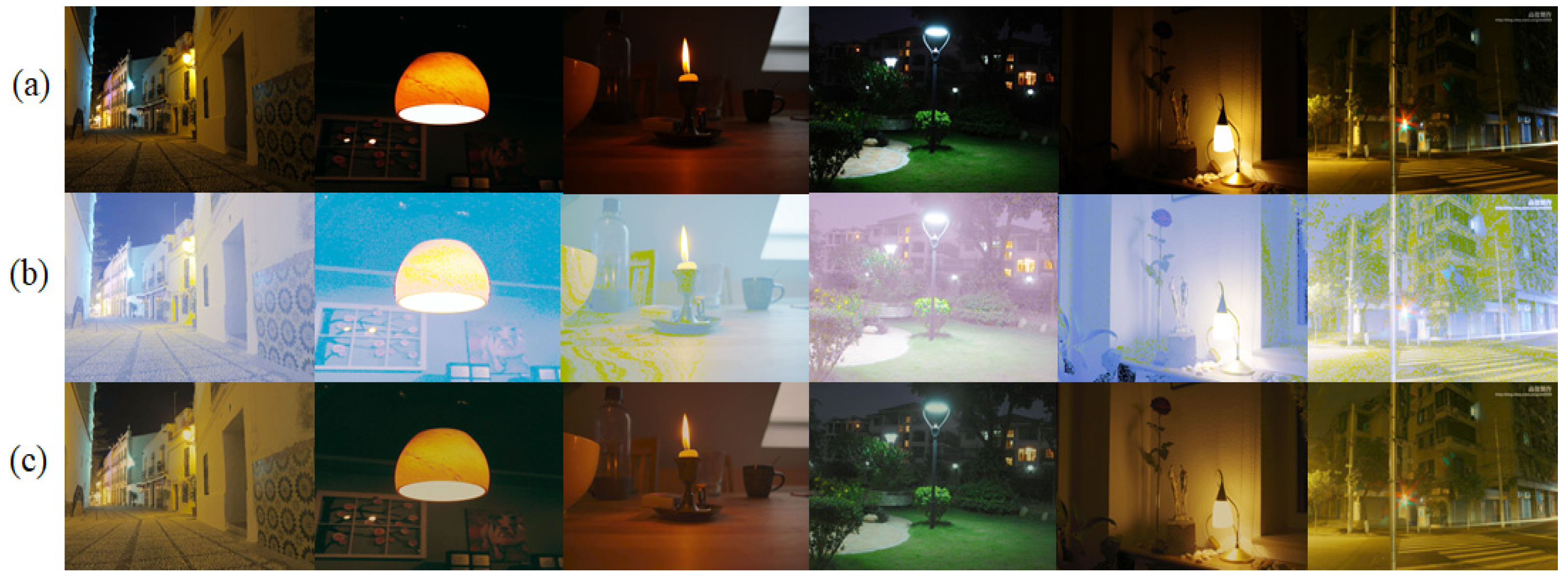
Using Equations (2)–(4), the stretched image has no overflow and appears natural. Figure 1a shows the low-light input image, Figure 1b shows the image stretched using the gamma correction method, and Figure 1c shows the image initially stretched using the adaptive ellipse. As shown in Figure 1, the image stretched using gamma correction has hazy features and features a color shift; however, the adaptive ellipse is able to stretch the low-light images naturally and does not show overflow in either the low-intensity regions or the bright-intensity regions. The stretching performance of Equations (2)–(4) is shown in Figure 1.

Sometimes, in excessive dark images, the stretched image still has a low level of intensity. Therefore, this paper proposes the use of a second enhancement step based on an image-adaptive mask (IAM) and reversed color channel. Excessively dark images have a low intensity value that is close to zero. Therefore, to stretch these images, an IAM is needed. An IAM is composed of reverse channels and the initially stretched image. If the image is dark, its color channel will be dark, whereas its reverse channel will be bright. Though the image is dark, the bright regions caused by the flash of the camera are in the reverse channel, and the bright region will have a value of zero. Because of this, the IAM is able to enhance low-light images naturally in both the excessively low-intensity regions and in the high-intensity regions. The IAM procedure can be described as:

$$I_M^c\left(x\right)=\left(1-I^c\left(x\right)\right)·I_{IE}^c\left(x\right){,}^{}$$

(5)

where $I_M^c\left(x\right)$ is the image-adaptive mask image, $I_{IE}^c\left(x\right)$ is the initial stretched image, $x$ is the location of the pixel, and $c\in \left\{r,g,b\right\}$. Although the bright regions of low-light images contain minority components, because these have neither symmetry nor asymmetry in their distribution, the bright region will be controlled using the image-adaptive mask, $I_M^c\left(x\right).$ Using Equation (5), extremely dark images can be compensated for by the initial adaptive image, $I_{IE}^c\left(x\right)$, and reverse images.

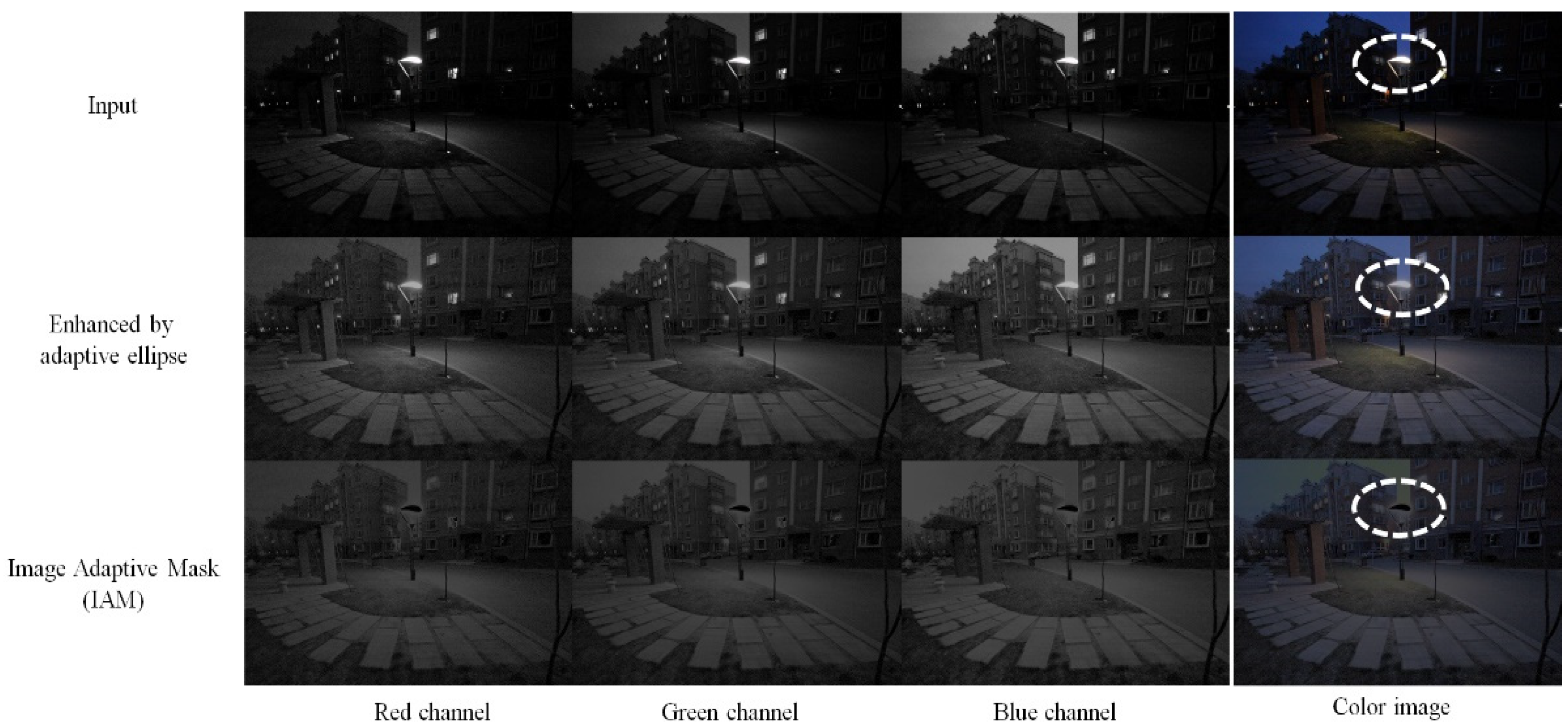
Figure 2 shows the input image stretched using the adaptive ellipse and image-adaptive mask (IAM). As shown in Figure 2, the image stretched using the adaptive ellipse has higher contrast than the input image. The IAM shows the dark and bright regions (due to lamp lightness) and is able to maintain the stretched region using an adaptive ellipse (the white dotted circle indicates the variation of light area). By this point, because the bright region turns dark, as shown in Figure 2, it prohibits the over-enhancement of parts of images.

However, these regions can overflow when the IAM and input images are directly in the bright region. Thus, the adaptive combination procedure is needed. The combined procedure using the input image and the IAM consists of summing the measurements. The combination step can be described as:

$$I_E^c\left(x\right)={\delta }_0^{}·I^c\left(x\right)+{\delta }^c·I_M^c\left(x\right){,}^{}$$

(6)

$${\delta }_0^{}=\sqrt{\frac{{{\displaystyle \sum }}_c\underset{c}{max}\left(I^c\left(x\right)\right)}{3}}{,}^{}$$

(7)

$${\delta }^c=\frac{m\left(I_M^c\right)}{m\left(I^c\right)}{,}^{}$$

(8)

where $I_E^c\left(x\right)$ is the enhanced image, ${\delta }_0^{}$ is the squared root mean value of the maximum value of the color channels, and ${\delta }^c$ is the ratio between the mean value of the masked image and the mean value of the input image. Using Equation (6), low-light images can be enhanced in a way that appears natural, maintains the features of the original image, and reflects the image’s features using an image-adaptive mask through the image adaption ratio, ${\delta }_0^{},{\delta }_{}^c$. Though low-light images have a low intensity value, the maximum intensity values of the color channels are not zero due to the light source. Therefore, to control the channel’s intensity value, the mean value of the adaptive channel’s maximum pure mean value is used; it can be applied to an input image using Equation (7). Moreover, to apply the IAM image adaptively, this paper uses the ratio of the input and IAM images as an adaptive measure, ${\delta }^c$. If the input image is darker, the mask image will be brighter, and, as a result, the ${\delta }^c$ will be bigger, and vice versa. Equations (5) and (6) are similar to the WB method [29]. The difference is that the WB method [29] uses one channel to improve the image. However, the color channels of low-light images are uniform and have a low level of intensity. Therefore, to enhance low-light images, high-intensity color channels are needed. Therefore, this paper improves low-light images using adaptive ellipse through guiding images such as mask images. Moreover, overflow can be prevented using an image-adaptive measure. This is described as:

$$I_A^c\left(x\right)={\delta }_A^c·I_E^c\left(x\right){,}^{}$$

(9)

$${\delta }_A^c=\frac{1}{\underset{c}{max}(I_E^c\left(x\right))}{,}^{}$$

(10)

where $I_A^c\left(x\right)$ is an image that has been subjected to the adaptive measure ${\delta }_A^c$. If the channel overflows, the maximum value will be above one. Therefore, the maximum value of the enhanced image’s color channel will be reversed to adjust the intensity of each color channel. Using Equations (9) and (10), the enhanced image will look natural and no overflow will be present.

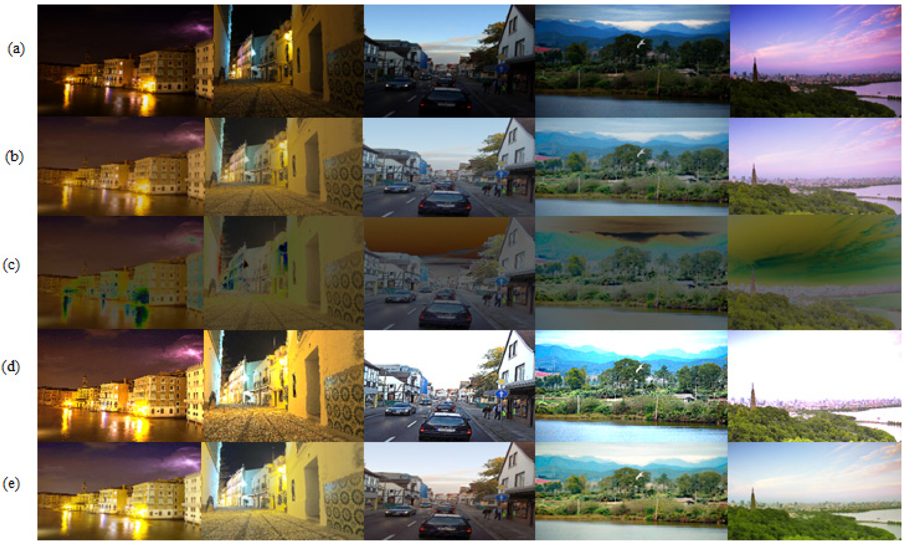
Figure 3 shows the (a) input images; (b) initial stretched images; (c) IAM images; (d) images enhanced without IAM, which contain overflow regions; and (e) images enhanced with IAM, which have no overflow regions.

As shown in Figure 3, the proposed method can achieve a suitable performance in enhancing low-light images. In particular, in the enhanced image shown in the fifth column, the proposed method enhances both the image’s intensity value and color components in a way that seems natural.

When a low-light image is enhanced, the image’s noise components will also be increased, resulting in the enhanced image looking dim and hazy. Therefore, to obtain refined images, this paper uses a guided image filter [28], which can be described as:

$$I_G^c\left(x\right)=GF\left\{I_A^c\left(x\right),K,EPS\right\}{,}^{}$$

(11)

$$I_{GE}^c\left(x\right)=\left(I_A^c\left(x\right)-I_G^c\left(x\right)\right)·{\alpha }^c+I_G^c\left(x\right){,}^{}$$

(12)

where $GF\{.\}$ is the guided filter, $K$ is the kernel size that is set to 2, and the $EPS$ is set to ${0.4}^2$. $I_G^c\left(x\right)$ is the guided image, $I_{GE}^c\left(x\right)$ is the image that has been enhanced using the guided filter, and ${\alpha }^c$ is the enhancement measure used. Using Equations (11) and (12), the improved hazy particles can be suppressed and the enhanced image will appear natural and clear. When low-light images are enhanced, because the noise components are also increased, an image-adaptive enhancing measure is needed to obtain an enhanced image that appears natural, and this is represented as ${\alpha }^c$. To obtain this measure, this paper uses a combination of triple ratio, as with ${\alpha }_r^c$. The first is the ratio of the enhanced image and the input image. If the image is enhanced further, the noise components will also be enhanced further. The second ratio is the IAM and the input image. The IAM also relatively enhances the input image. The third ratio is the initial enhanced image and the input image. The three terms are combined with the squared sum as shown below:

$${\alpha }_r^c=\sqrt{\frac{m\left(I_A^c\right)}{m\left(I^c\right)}+\frac{m\left(I_M^c\right)}{m\left(I^c\right)}+\frac{m\left(I_{IE}^c\right)}{m\left(I^c\right)}}{.}^{}$$

(13)

$${\alpha }_{}^c=\frac{{\alpha }_r^c+{\alpha }_0}{2}{.}^{}$$

(14)

where${\alpha }_{}^c$ is the image-adaptive measure; ${\alpha }_r^c$ is the image-adaptive ratio; and ${\alpha }_0$ is the initial value, which is set to 5. Using Equations (11)–(14), the enhanced low-light image can be refined adaptively. The low-light image is enhanced in a way that appears natural with regard to both its low intensity and haze particles. Moreover, the image’s color can also be balanced by the proposed method. Therefore, the proposed method has a good performance for both low-light image enhancement and image color balancing.

3. Results and Discussion

Low-light images are obtained under circumstances where there is insufficient light and appear dim and dark. To enhance these images, this paper uses IAM. To evaluate the performance of the proposed method subjectively and objectively, seven state-of-the-art methods (low-light image enhancement using illumination map estimation (LIME) [9], low-light image enhancement using the camera response model (LECARM) [12], weakly illuminated image enhancement using a convolutional neural network (LLINet) [23], the naturalness preserved enhancement algorithm (NPE) [8], and low-light image enhancement using the dehazing algorithm (LVED) [19], low light image enhancement with semi decoupled decomposition (LISD) [20], and bio inspired multi exposure fusion framework [6]), and seven databases (LIME [9], NPE [8], NPE ex1 [8], NPE ex2 [8], NPE ex3 [8], MEF [6], and Exdark [30]) are used under various circumstances. The LIME dataset is used in [9], and it contains 10 low-light images [6,9]. The NPE dataset is used in [8], and it contains eight images [6,8]. The NPE external datasets, NPE ex1, NPE ex2, and NPE ex3, contain low-light scenes captured during cloudy days or at night [6,8]. The MEF dataset has 17 images [6], and the exclusively dark (Exdark) dataset [30] has 7363 images. In this paper, to compare the existing methods with the proposed method, we select 1200 images from the Exdark dataset [30]. To evaluate the results objectively, various measures are used.

Table 1. Descriptions of dataset [6,8,9,30].

Datasets	Descriptions
MEF [6]	17 real-world images, including indoor and outdoor views
LIME [9]	10 natural low-light images
NPE [8]	85 low-light images with four categories; NPE, NPE ex1, NPE ex2, and NPE ex3
ExDark [30]	12 categories, 7363 images This paper uses 1200 images; 100 images were selected from each of the 12 categories

shows the descriptions of various datasets [6,8,9,30]. As shown in Table 1, to compare the proposed method with the existing methods, images obtained under various conditions are used. In particular, because the ExDark dataset [30] has 7363 images across 12 categories, this paper chooses 1200 images by selecting 100 images from each of the 12 categories.

• Subjective Comparison

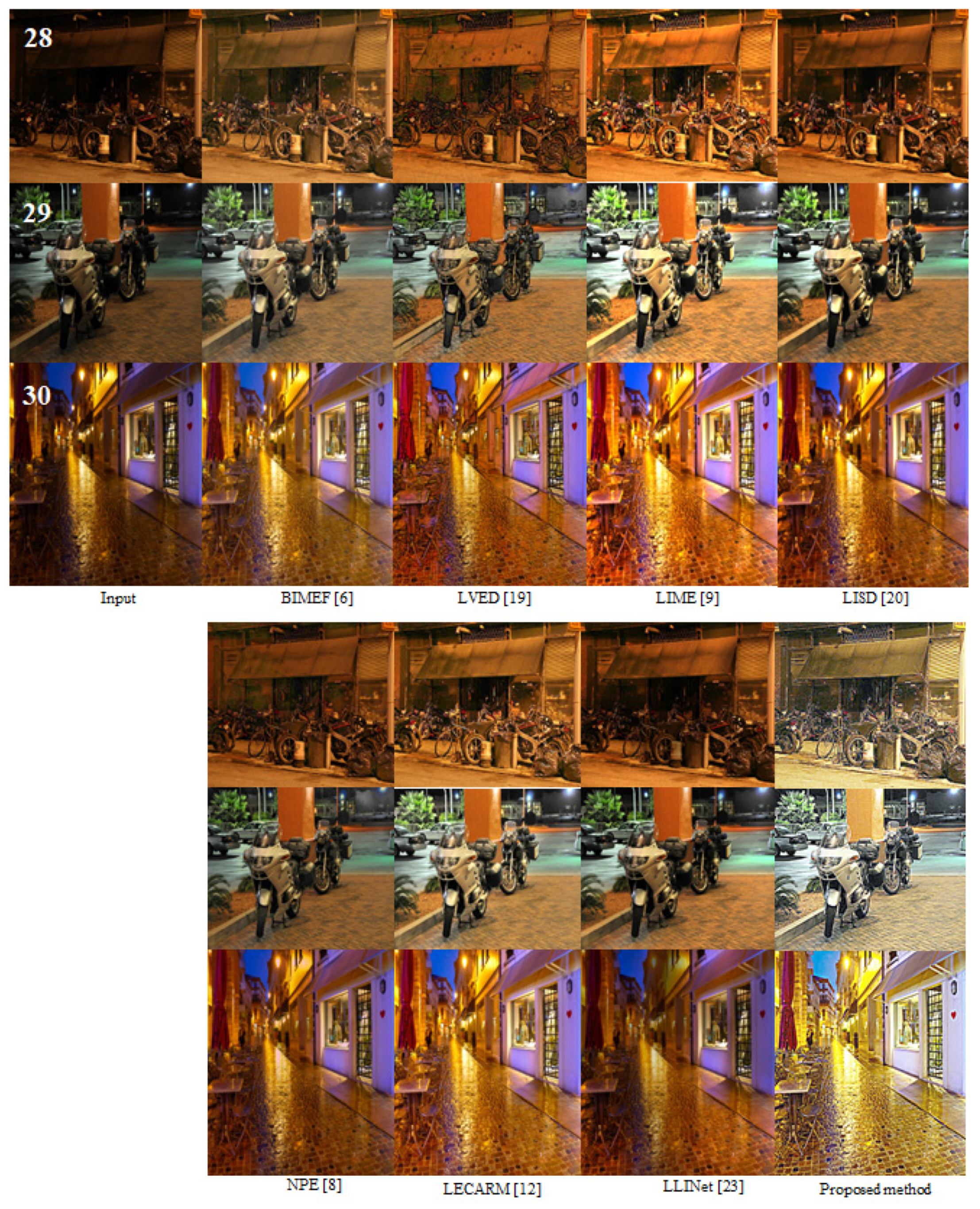
In this research, we created a low-light image enhancement method that uses an image-adaptive mask and guided image filter [28]. The proposed method demonstrated a good performance in enhancing low-light images. This section shows a subjective performance comparison of the proposed method with existing state-of-the-art methods such as BIMEF [6], LVED [19], LIME [9], LECARM [12], LLINet [23], and NPE [8], LISD [20] through Figure 4, Figure 5, Figure 6, Figure 7, Figure 8, Figure 9, Figure 10, Figure 11, Figure 12 and Figure 13. Each Figure shows three low-light images used as inputs before the images are enhanced using the state-of-the-art methods and the proposed methods are compared. The numbers with white color in Figure 4, Figure 5, Figure 6, Figure 7, Figure 8, Figure 9, Figure 10, Figure 11, Figure 12 and Figure 13 refer to the index of the image number in order.

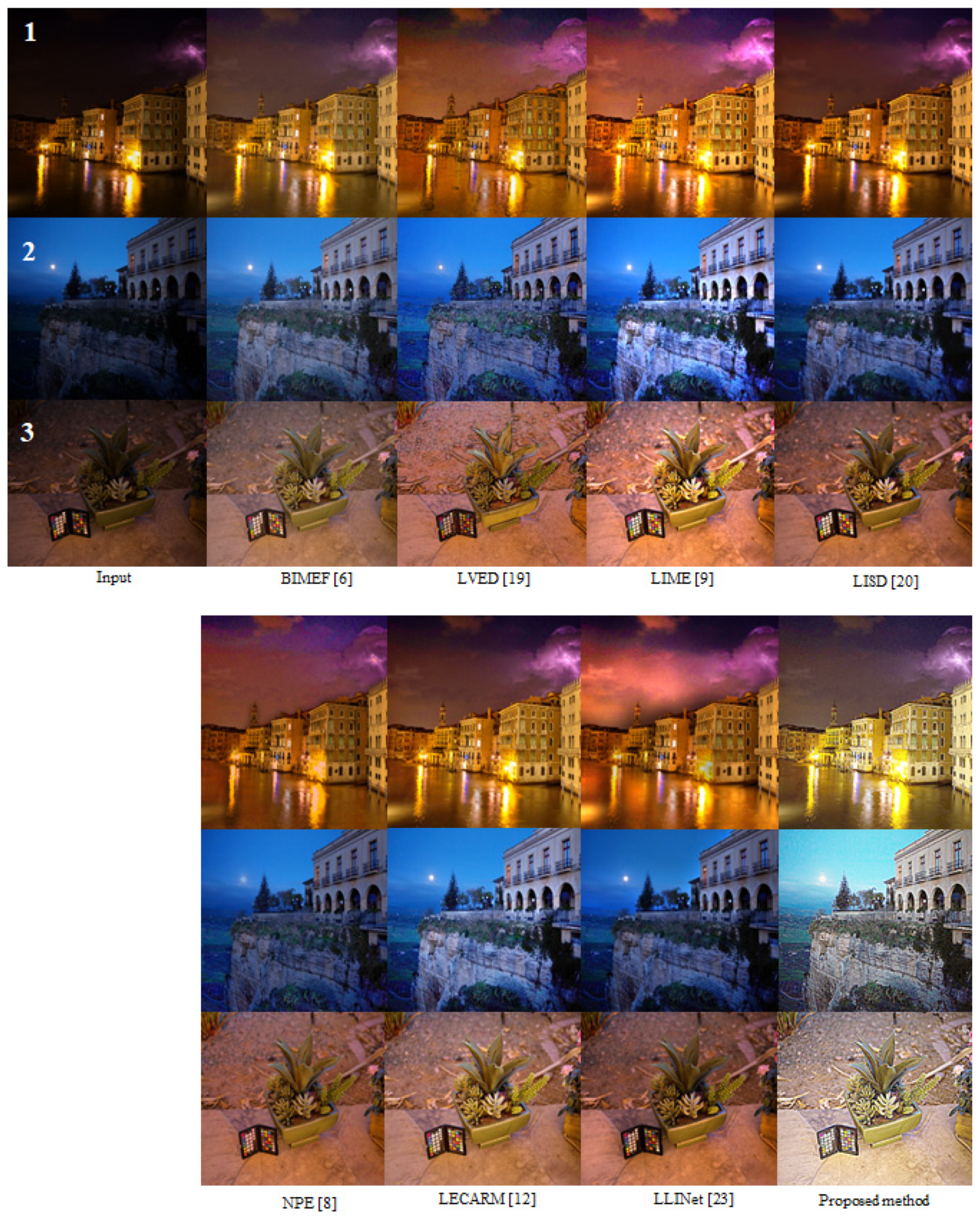
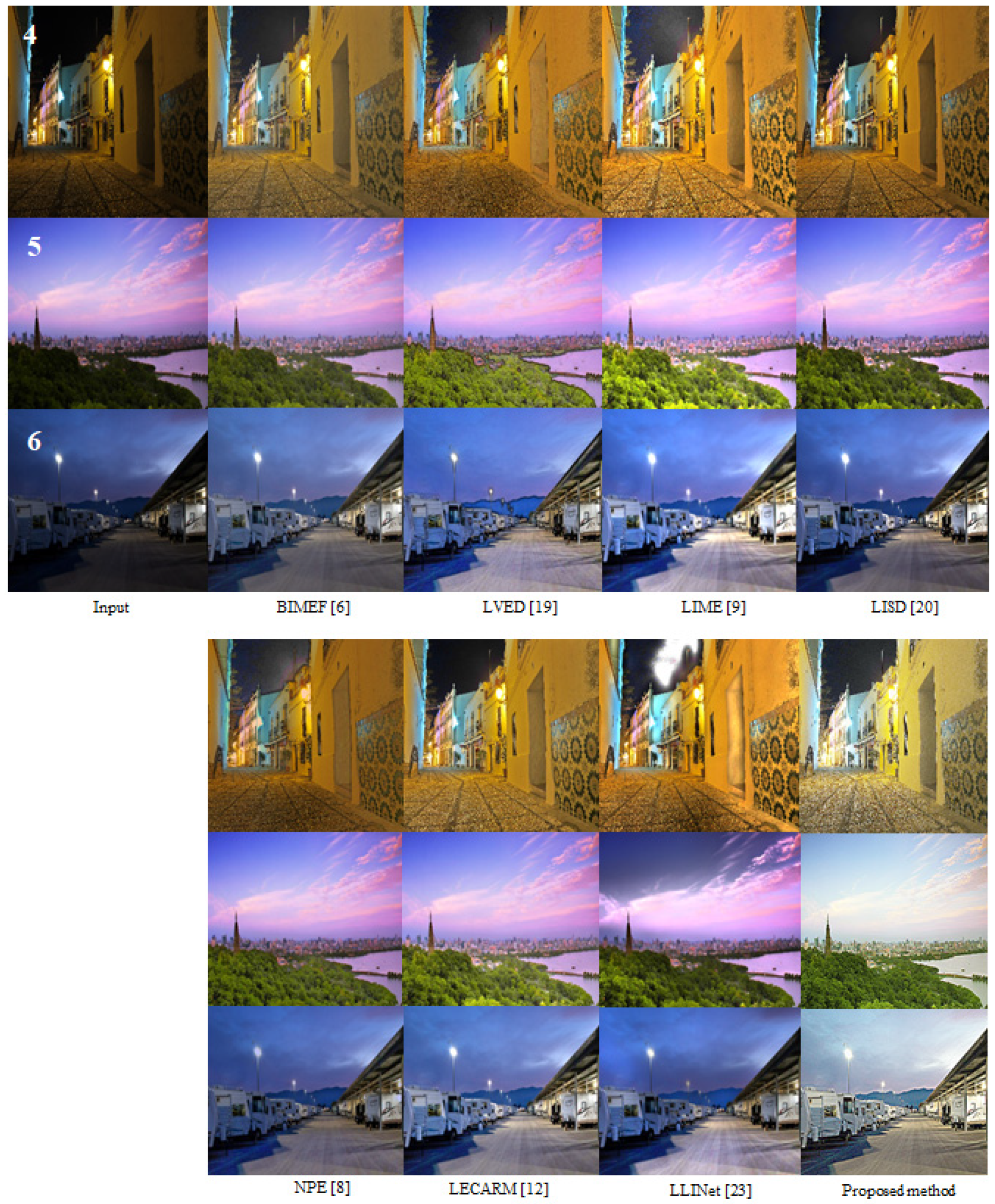
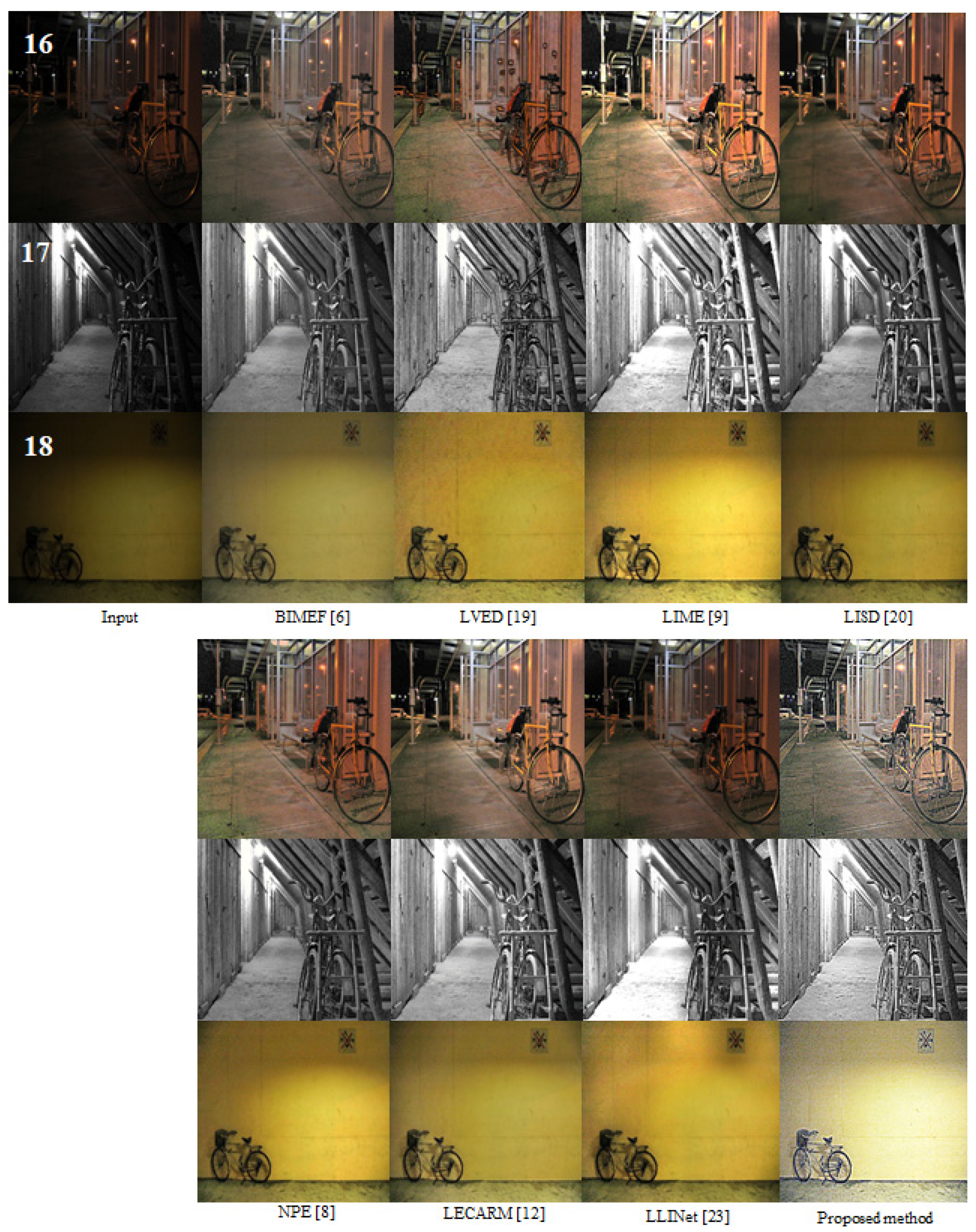
Figure 4, Figure 5 and Figure 6 show the experimental results obtained using the LIME [9], NPE [8], and MEF [6] databases. The LVED method [19] over-enhanced the images, and an artifact effect can be observed in the sharp edge region. The LIME method [9] produced images that appear unnatural due to over-enhancement: the river region is over-enhanced, as is the area reflected by the lamp light. The LISD method [20] enhances the low light image without over-enhancement area and distortion. The NPE method [8] enhanced the low-light images unnaturally, especially in the sharp edge regions, and in the light-reflected areas of the river, a ringing effect occurred. Additionally, the colors in the lamp-lit regions look dimmer. The LECARM method [12] enhanced the low-light images naturally, and no color shift occur. The LLINet method [23] enhanced the low-light images in a way that appeared unnatural in some regions of the image, such as in bright and boundary regions; in other words, a ringing effect occurred in the edge regions. However, no color shift occurs. The proposed method enhanced the low-light images naturally in both the edge regions and the reflectance areas. Moreover, in some cases, the proposed method reflected the image’s features well, such as its color. While the low-light images were enhanced, the proposed method, which balanced the images’ color channels well, produced images that looked natural and had natural colors.

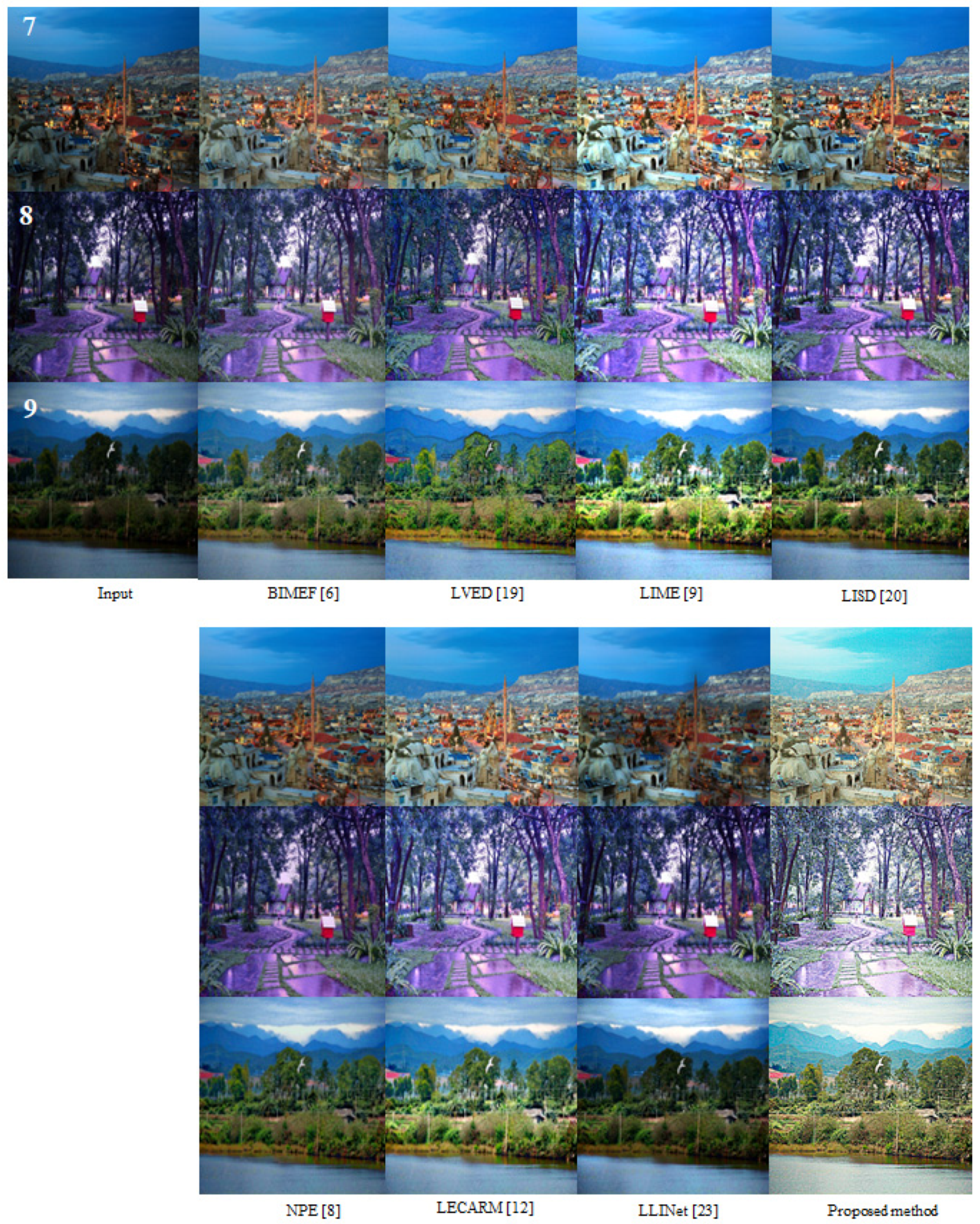
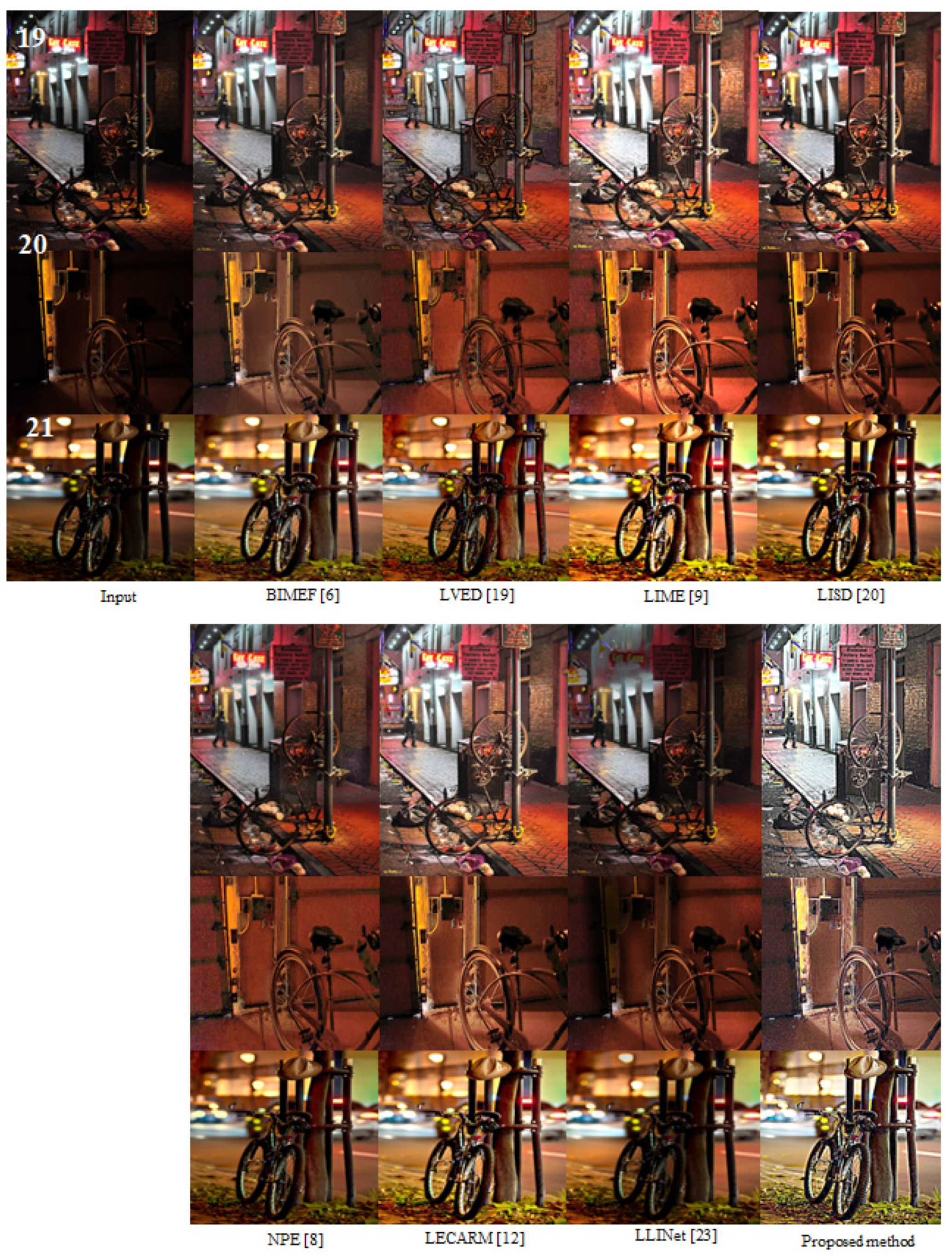
Figure 7, Figure 8 and Figure 9 show the results obtained using the existing methods and the proposed method based on images from the LIME [9], NPE [8], MEF [6], and Exdark [30] databases. The LVED method [19] showed an artifact effect in sharp edge regions. The LIME method [9] was able to make the pictures look natural. However, this method leads to over-enhancement. The LISD method [20] enhances the low light image but, the dark area does not improve efficiency as it does with a light house. The NPE method [8] is able to enhance low-light images naturally in both dark and bright areas. The LECARM method [12] is able to enhance low-light images in a way that appears natural. The LLINet method [23] enhances low-light images in a way that appears unnatural, struggling to deal with bright regions. The proposed method is able to enhance low-light images in a way that appears natural, especially in edge regions, dark regions, and bright areas.

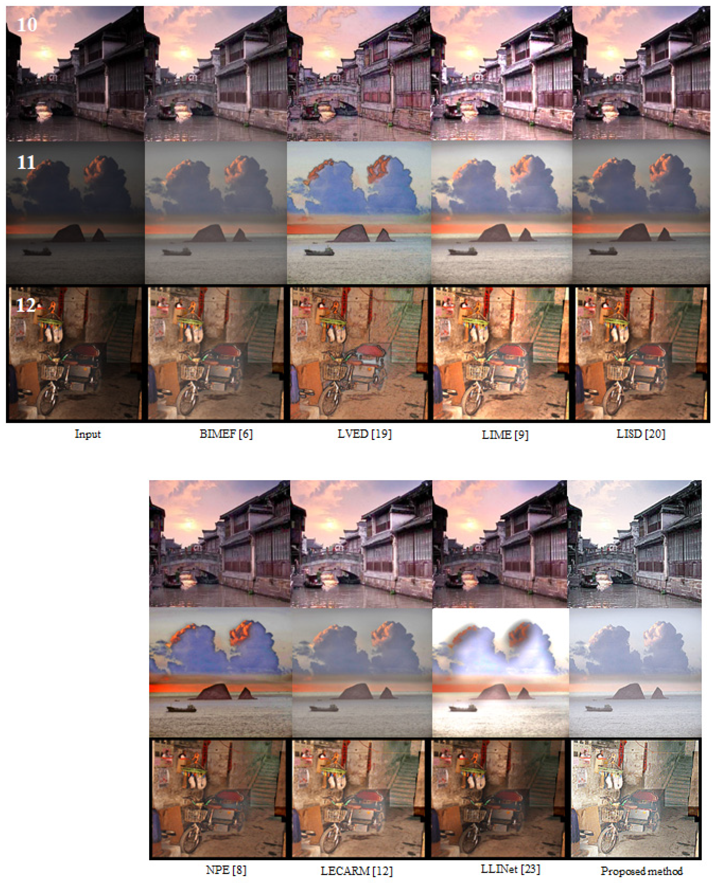
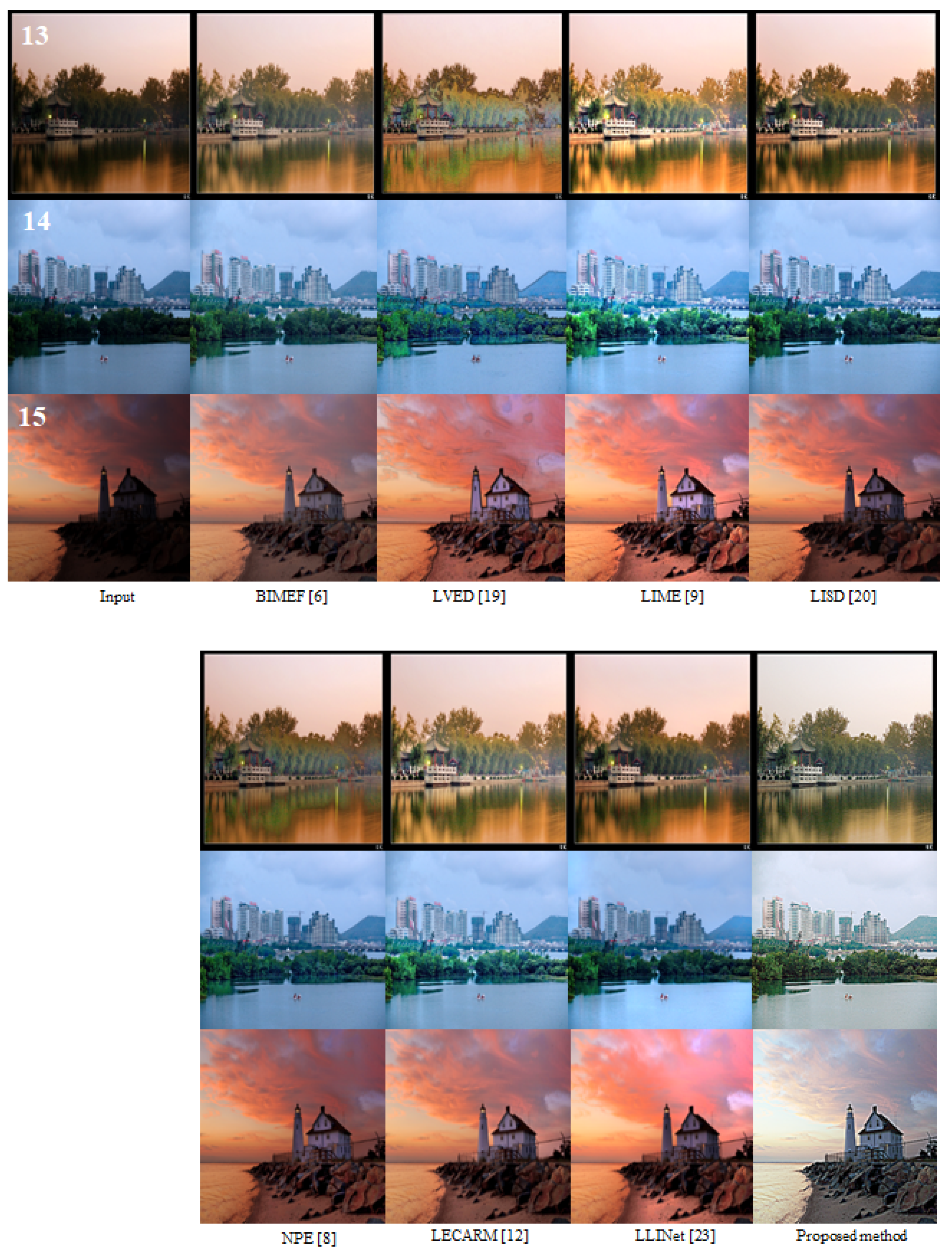
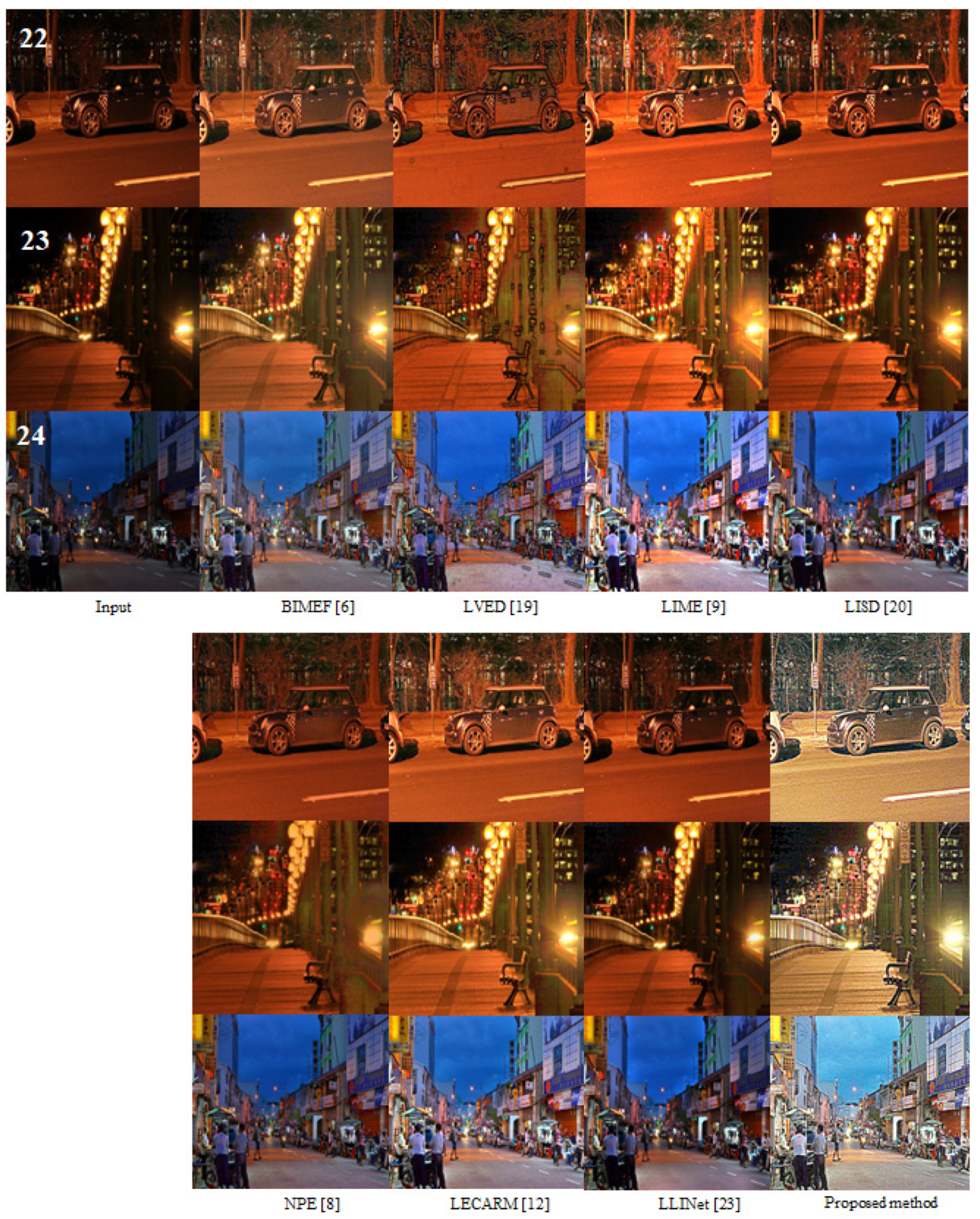
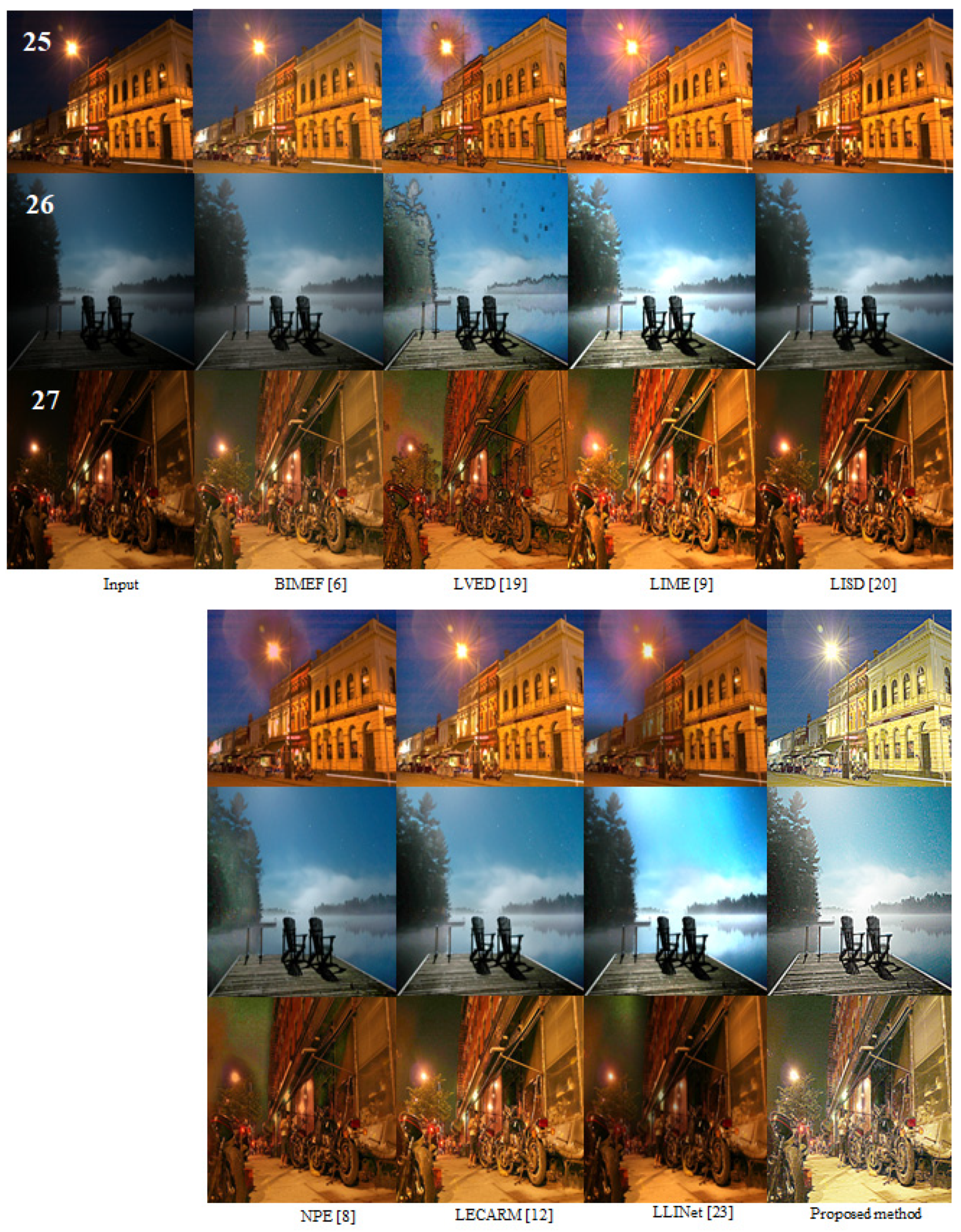
Figure 10, Figure 11, Figure 12 and Figure 13 show the results obtained using the existing methods and the proposed method based on images from the Exdark [30] database. The LVED method [19] over-enhanced the images and created an artifact effect in sharp edge regions. In particular, the edge lines of the building look unnatural due to over-enhancement. Additionally, a ringing effect occurred in the boundary regions. The LIME method [9] produced images that appeared unnatural due to over-enhancement. In particular, a ringing effect occurred around the boundaries of the buildings and the leaf regions were too bright. The LISD method [20] enhances the low light image without distortion. The LISD method [20] enhances the low light image but, the dark area is not improved sufficiently. The NPE method [8] enhanced low-light images in a way that appeared unnatural. For example, the ringing effect occurred around the boundary region of the building and there was a blocked area in the sky due to over-enhancement. The LECARM method [12] was able to enhance low-light images in a way that appeared natural, and no color shift occurred. The LLINet method [23] enhanced the low-light images in a way that appeared unnatural, especially in boundary regions. In other words, a ringing effect was visible in edge regions. The proposed method was able to enhance low-light images naturally in both the edge regions and in bright areas.

As shown in Figure 4, Figure 5, Figure 6, Figure 7, Figure 8, Figure 9, Figure 10, Figure 11, Figure 12 and Figure 13, the enhanced image using some methods showed a ringing effect that occurred due to over-enhancement between the boundary area and the dark region. Meanwhile the proposed method was able to improve the low-light images without causing a ringing effect. Additionally, the proposed method was able to reflect aspects of the images such as time, light conditions, and reflection.

Although low-light images are taken in dark conditions, the environment of each image has unique features. Therefore, to enhance low-light images in a way that appears natural, the images’ features should be reflected. However, the existing methods only improve the intensity of the image, creating images that appear unnatural. Meanwhile, the proposed method improves low-light images by maintaining their features as with sunsets, which have a reddish color and specific time. If the sunset is starting, then the image is lightly reddish. Furthermore, if the sunset has climaxed, the image is mostly reddish and dark. This paper reflects the image’s time naturally. Therefore, the performance of the proposed method is superior to that of state-of-the-art methods.

2.

Objective Comparison

A subjective comparison of enhanced low-light images obtained using the proposed method and existing state-of-the-art methods is shown in Figure 4, Figure 5, Figure 6, Figure 7, Figure 8, Figure 9, Figure 10, Figure 11, Figure 12 and Figure 13. The performance of the proposed method is subjectively superior to that of the state-of-the-art methods. Because obtaining the ground truth in low-light images is not easy, no reference measure can be used to assess the enhancement of low-light images. To compare the performance of the proposed method and the existing method objectively, we used three measures: the contrast enhancement-based image quality (CEIQ) [31] measure, the underwater image quality measure (UIQM) [32], and the natural image quality evaluator (NIQE) [33]. The CEIQ [31] and UIQM [32] were used in any no reference image quality assessment. The NIQE [33] measure was used for low-light images that had been enhanced. The UIQM [32] is able to reflect the contrast, colorfulness, and sharpness of an image. Low-light images are dark and show an orange color shift due to light conditions similar to those seen in underwater images. Therefore, the UIQM [32] is a suitable measure with which to assess low-light images.

Table 2. Description of metrics [31,32,33].

Metrics	Description	Reference	Performance
NIQE [33]	Natural image quality evaluator; assessment of natural scene static model using multivariate Gaussian model (MGM)	No reference	The lower the better
CEIQ [31]	Contrast-enhancement-based image quality assessment	No reference	The higher the better
UIQM [32]	Underwater image quality measure; assesses the image’s colorfulness, sharpness, and contrast	No reference	The higher the better

provides descriptions of various metrics that can be used for objective comparisons. As shown in Table 2, the metrics had any no references because obtaining reference low-light images in the real world is difficult. Each metric reflects the image’s colorfulness, sharpness, and contrast. The lower the NIQE score [33] is, the better the image is enhanced and the higher the quality. If the CEIQ [31] and UIQM [32] scores are high, this indicates that the improved image is of good quality.

Table 3. Comparison of the CEIQ [31] score obtained in Figure 4, Figure 5, Figure 6 and Figure 7, in order (the higher the score is, the better the enhanced image is).

Image #	LVED [19]	LIME [9]	BIMEF [6]	NPE [8]	LECARM [12]	LISD [20]	LLINet [23]	PM
1	3.301	3.495	3.207	2.770	3.428	3.173	3.451	3.532
2	3.370	3.625	3.357	2.975	3.480	3.324	3.200	3.684
3	2.933	3.331	3.116	2.857	3.131	3.195	3.271	3.506
4	3.398	3.494	3.299	3.156	3.381	3.409	3.499	3.665
5	3.409	3.459	3.523	3.496	3.466	3.540	3.598	3.410
6	3.365	3.463	3.342	3.117	3.306	3.392	3.481	3.552
7	3.382	3.542	3.259	3.196	3.405	3.427	3.358	3.532
8	3.505	3.682	3.486	3.287	3.629	3.575	3.469	3.599
9	3.530	3.619	3.489	3.369	3.517	3.579	3.528	3.640
10	3.667	3.661	3.646	3.578	3.681	3.724	3.646	3.616
AVG	3.386	3.537	3.372	3.180	3.442	3.434	3.450	3.574

,

Table 4. Comparison of the CEIQ [31] score obtained for images shown in Figure 7, Figure 8, Figure 9 and Figure 10, in order (the higher the score is, the better the enhanced image is).

Image #	LVED [19]	LIME [9]	BIMEF [6]	NPE [8]	LECARM [12]	LISD [20]	LLINet [23]	PM
11	2.970	3.090	2.563	2.967	2.691	2.848	2.604	3.006
12	3.189	3.488	3.227	2.946	3.301	3.360	3.129	3.543
13	3.401	3.481	3.474	3.371	3.486	3.532	3.350	3.477
14	3.235	3.233	3.359	3.399	3.248	3.316	3.125	3.229
15	3.235	3.390	3.425	3.287	3.395	3.515	3.432	3.545
16	3.356	3.655	3.179	3.157	3.467	3.180	2.994	3.593
17	3.660	3.497	3.502	3.467	3.588	3.591	3.610	3.600
18	2.680	3.431	2.923	3.195	2.989	3.018	2.987	3.352
19	3.472	3.654	3.371	3.216	3.641	3.507	3.099	3.587
20	3.080	3.361	2.923	2.685	2.967	2.895	2.750	3.334
AVG	3.228	3.428	3.195	3.169	3.277	3.276	3.108	3.427

,

Table 5. Comparison of the CEIQ [31] scores obtained for images shown in Figure 10, Figure 11, Figure 12 and Figure 13, in order (the higher the score is, the better the enhanced image is).

Image #	LVED [19]	LIME [9]	BIMEF [6]	NPE [8]	LECARM [12]	LISD [20]	LLINet [23]	PM
21	3.517	3.656	3.530	3.317	3.618	3.542	3.273	3.580
22	3.164	3.392	3.225	2.812	3.268	3.187	3.056	3.637
23	3.249	3.497	3.320	2.895	3.400	3.294	3.019	3.614
24	3.440	3.647	3.275	3.072	3.510	3.373	3.330	3.560
25	3.306	3.452	3.324	3.027	3.344	3.407	3.223	3.567
26	3.445	3.714	3.373	3.269	3.600	3.553	3.686	3.628
27	3.335	3.587	3.345	2.999	3.497	3.322	3.116	3.657
28	3.388	3.653	3.434	2.977	3.524	3.353	3.198	3.656
29	3.484	3.652	3.420	3.230	3.526	3.512	3.548	3.606
30	3.368	3.537	3.323	3.142	3.418	3.408	3.232	3.670
AVG	3.370	3.579	3.357	3.074	3.471	3.395	3.268	3.618

,

Table 6. Comparison of the UIQM [32] scores obtained for images shown in Figure 4, Figure 5, Figure 6 and Figure 7, in order (the higher the score is, the better the enhanced image is).

Image #	LVED [19]	LIME [9]	BIMEF [6]	NPE [8]	LECARM [12]	LISD [20]	LLINet [23]	PM
1	1.664	1.632	1.394	1.516	1.560	1.286	1.547	2.067
2	1.647	1.629	1.521	1.636	1.627	1.647	1.642	1.737
3	1.719	1.725	1.498	1.631	1.664	1.600	1.644	1.970
4	1.550	1.525	1.336	1.473	1.450	1.348	1.500	1.775
5	1.291	1.261	1.109	1.199	1.196	1.164	1.228	1.506
6	1.594	1.583	1.330	1.502	1.511	1.457	1.495	1.849
7	1.649	1.629	1.546	1.627	1.619	1.630	1.590	1.915
8	1.679	1.654	1.733	1.761	1.697	1.762	1.751	1.435
9	1.754	1.756	1.575	1.710	1.720	1.701	1.647	1.920
10	1.482	1.458	1.412	1.432	1.454	1.500	1.452	1.523
AVG	1.603	1.585	1.445	1.549	1.550	1.510	1.550	1.770

,

Table 7. Comparison of the UIQM [32] scores obtained for images shown in Figure 7, Figure 8, Figure 9 and Figure 10, in order (the higher the score is, the better the enhanced image is).

Image #	LVED [19]	LIME [9]	BIMEF [6]	NPE [8]	LECARM [12]	LISD [20]	LLINet [23]	PM
11	1.092	0.928	0.662	1.058	0.725	0.706	0.907	1.037
12	1.782	1.750	1.575	1.652	1.669	1.722	1.684	1.859
13	1.493	1.333	1.166	1.279	1.262	1.347	1.320	1.583
14	1.389	1.369	1.216	1.297	1.319	1.282	1.293	1.654
15	1.488	1.463	1.164	1.350	1.355	1.198	1.365	1.838
16	1.845	1.846	1.674	1.797	1.826	1.703	1.834	1.782
17	1.869	1.707	1.702	1.777	1.757	1.754	1.767	1.562
18	1.863	1.949	1.445	1.787	1.736	1.378	1.699	2.092
19	1.909	1.890	1.858	1.888	1.889	1.932	1.972	1.631
20	2.076	2.010	1.743	1.883	1.963	1.772	1.978	1.967
AVG	1.681	1.625	1.421	1.577	1.550	1.479	1.582	1.701

,

Table 8. Comparison of the UIQM [32] score obtained for images shown in Figure 10, Figure 11, Figure 12 and Figure 13, in order (the higher the score is, the better the enhanced image is).

Image #	LVED [19]	LIME [9]	BIMEF [6]	NPE [8]	LECARM [12]	LISD [20]	LLINet [23]	PM
21	1.795	1.869	1.587	1.691	1.776	1.857	1.717	1.871
22	2.004	1.940	1.752	1.882	1.888	2.043	1.995	1.771
23	1.816	1.757	1.575	1.725	1.722	1.742	1.788	1.937
24	1.824	1.793	1.593	1.745	1.729	1.732	1.751	1.899
25	1.752	1.683	1.482	1.645	1.620	1.577	1.595	1.925
26	1.489	1.498	1.214	1.396	1.367	1.247	1.513	1.827
27	1.902	1.924	1.692	1.860	1.873	1.874	1.869	1.869
28	1.993	2.016	1.747	1.920	1.965	2.036	1.970	1.822
29	1.858	1.876	1.698	1.808	1.797	1.828	1.827	1.862
30	1.698	1.681	1.589	1.649	1.652	1.661	1.616	1.781
AVG	1.813	1.804	1.593	1.732	1.739	1.760	1.764	1.856

,

Table 9. Comparison of the CEIQ [31] and UIQM [32] scores obtained for images shown in Figure 4, Figure 5, Figure 6, Figure 7, Figure 8, Figure 9, Figure 10, Figure 11, Figure 12 and Figure 13 [6,8,9,30] (the higher the score is, the better the enhanced image is).

	LVED [19]	LIME [9]	BIMEF [6]	NPE [8]	LECARM [12]	LISD [20]	LLINet [23]	PM
CEIQ [31]	3.328	3.515	3.308	3.141	3.397	3.368	3.275	3.539
UIQM [32]	1.699	1.671	1.486	1.619	1.613	1.583	1.632	1.776

,

Table 10. Comparison of the CEIQ [31] scores (datasets [6,8,9,30]) (the higher the score is, the better the enhanced image is).

	LVED [19]	LIME [9]	BIMEF [6]	NPE [8]	LECARM [12]	LISD [20]	LLINet [23]	PM
LIME [9]	3.208	3.483	3.143	3.031	3.229	3.150	3.229	3.402
NPE [8]	3.484	3.485	3.480	3.457	3.476	3.488	3.450	3.502
NPE ex1 [8]	3.307	3.345	3.268	3.283	3.285	3.338	3.298	3.388
NPE ex2 [8]	3.475	3.482	3.417	3.402	3.461	3.472	3.431	3.481
NPE ex3 [8]	3.401	3.427	3.331	3.310	3.390	3.386	3.386	3.408
MEF [6]	3.282	3.441	3.109	3.183	3.190	3.152	3.333	3.364
Exdark [30]	3.119	3.321	3.038	2.972	3.084	3.052	3.037	3.289

and

Table 11. Comparison of the UIQM [32] scores (datasets [6,8,9,30]) (the higher the score is, the better the enhanced image is).

	LVED [19]	LIME [9]	BIMEF [6]	NPE [8]	LECARM [12]	LISD [20]	LLINet [23]	PM
LIME [9]	1.625	1.595	1.443	1.552	1.558	1.507	1.572	1.706
NPE [8]	1.457	1.444	1.319	1.37	1.392	1.401	1.409	1.653
NPE ex1 [8]	1.482	1.439	1.343	1.430	1.394	1.388	1.439	1.530
NPE ex2 [8]	1.454	1.415	1.280	1.377	1.354	1.352	1.378	1.578
NPE ex3 [8]	1.600	1.526	1.460	1.510	1.504	1.516	1.552	1.618
MEF [6]	1.559	1.522	1.354	1.459	1.475	1.341	1.451	1.727
Exdark [30]	1.677	1.626	1.488	1.576	1.615	1.577	1.595	1.689

show the values obtained for the CEIQ [31] and UIQM [32] measurements shown in Figure 4, Figure 5, Figure 6, Figure 7, Figure 8, Figure 9, Figure 10, Figure 11, Figure 12 and Figure 13, representing all datasets. Table 3, Table 4 and Table 5 show the CEIQ [31] measurements provided in Figure 4, Figure 5, Figure 6, Figure 7, Figure 8, Figure 9, Figure 10, Figure 11, Figure 12 and Figure 13. If the image is enhanced well, then the CEIQ [31] will have a high score.

Table 3 shows a comparison of the CEIQ [31] scores obtained for the existing methods and for the proposed method for the images shown in Figure 4, Figure 5, Figure 6 and Figure 7 in order. A higher CEIQ [31] score indicates that the enhanced image is better. The LIME method [9] obtained the brightest images among all the existing methods for the images shown in Figure 4, Figure 5, Figure 6 and Figure 7; its CEIQ [31] score was therefore high because the CEIQ measure indicates the contrast of an image. The LISD method [20] has a lower CEIQ score than the LIME method [9] in some images because the CEIQ measure reflects the image’s contrast. The NPE and LECARM methods [8,12] produced images that were less bright than those produced using the LIME method [9] and obtained lower CEIQ [31] scores than the LIME method [9] because the contrast of their enhanced images was lower than that of images enhanced using the LIME method [9]. The proposed method produced enhanced images that appeared natural, and its CEIQ [31] score was higher than those obtained by the existing methods.

Table 4 shows the comparison of the CEIQ [31] scores obtained by the existing methods and the proposed method for the images shown in Figure 7, Figure 8, Figure 9 and Figure 10 in order. The LIME method [9] obtained the brightest images among the existing methods, and its CEIQ [31] score was higher than the score obtained by the other methods because the CEIQ measure reflects the contrast of an image. The LVED method [19] led to an artifact effect in the edge regions, and this method achieved a the lower CEIQ [31] score than the LIME [9] method did because the contrast of the images enhanced using the LVED method [19] was lower than that of the images enhanced using the LIME method [9]. The enhanced image using the LISD method [20] has a lower CEIQ score than the LIME method [9] because the enhanced image using the LIME method [9] has an overflowed area and these are bright. The enhanced image using the NPE method [8] has lower CEIQ score than LECARM method [12]. Though the LECARM method [12] enhanced the images better than the NPE method did [8], the CEIQ [31] score obtained by the LECARM method [12] was higher than that obtained by the NPE method [8]. Because the LLINet method [23] produced over-enhanced regions, its CEIQ [31] score was lower than that of the NPE method [8]. The images that were enhanced using the proposed method showed natural-looking dark and bright regions, and its CEIQ [31] score was also higher than that of the LVED [19] method, as the CEIQ score reflects the contrast of an image.

Table 5 shows the CEIQ [31] scores obtained using the existing methods and the proposed method for the images shown in Figure 10, Figure 11, Figure 12 and Figure 13 in order. The LVED method [19] led to a ringing effect in edge regions, and its CEIQ [31] score was lower than that of the LIME [9] method because the images enhanced using the LIME method [9] were brighter than those enhanced using the LVED method [19]. Though the LIME method [9] produced over-enhanced regions and a ringing effect, its CEIQ [31] score was higher than that of the NPE method [8] in some images because the CEIQ score reflects the contrast of an image. The NPE method [8] showed the lowest CEIQ [31] value among all of the compared methods for some images. The LISD method [20] has a higher CEIQ score than the NPE method [8] because the CEIQ measure reflects the image’s contrast. The LECARM method [12] received a lower CEIQ [31] value than the LIME method [9]. The LLINet method [23] showed a ringing effect in boundary regions, but its CEIQ [31] score was higher than that of the NPE [8] method because the CEIQ score reflects the contrast of an image. Though the proposed method does not produce a ringing effect, its CEIQ [31] score was lower than that of the LIME [9] method for some images because the CEIQ reflects the contrast of an image. As shown by the CEIQ [31] scores, in some cases, even though no ringing effect was observed and the image was enhanced in a way that appeared natural, the CEIQ [31] score may not be the highest. The CEIQ [31] score is not a perfect measure for assessing enhanced low-light images because the CEIQ only reflects the contrast of an image.

Table 6, Table 7 and Table 8 show the UIQM [32] scores obtained for images shown in Figure 4, Figure 5, Figure 6, Figure 7, Figure 8, Figure 9, Figure 10, Figure 11, Figure 12 and Figure 13. The images were enhanced well, and the UIQM scores were high.

Table 6 shows the UIQM [32] scores obtained for images shown in Figure 4, Figure 5, Figure 6 and Figure 7 in order. The LVED method [19] produced a higher UIQM score than the other existing methods, even though in some enhanced images a ringing effect was visible. This is because the UIQM score reflects the sharpness, contrast, and colorfulness of an image. The LISD method [20] has a lower UIQM score than the LECARM method [12] because the UIQM measure reflects the image’s contrast, sharpness, and colorfulness. The LIME [9] method produced a lower UIQM [32] score than the LVED method [19], even though the images that were enhanced using this method were the brightest subjectively. This is because the UIQM score reflects the contrast, sharpness, and colorfulness of an image. The BIMEF [6] method received a lower UIQM [32] score than the LVED method [19], even though the enhanced images showed less of a ringing effect than those enhanced using the LVED method [19]. This is because the UIQM score reflects the contrast, sharpness, and colorfulness of an image. The NPE [8] method received a lower UIQM [32] score than the LVED method [19] because the UIQM measure consists of the image’s sharpness, contrast, and colorfulness. The LECARM [12] method has a higher UIQM [32] score than the BIMEF [6] method. The LLINet [23] method has a lower UIQM [32] score than the LVED method [19] because the UIQM score reflects the image’s contrast, colorfulness, and sharpness. Meanwhile, the proposed method has a higher UIQM [32] score than the other methods because the UIQM score consists of the image’s colorfulness, sharpness, and contrast.

Table 7 shows the UIQM [32] scores for Figure 7, Figure 8, Figure 9 and Figure 10 in order. The LVED method [19] has a higher UIQM [32] score than the other methods, though the images that were using this method have a visible ringing effect because the UIQM score measures an image’s sharpness, colorfulness, and contrast. The LISD method [20] has a lower UIQM score than LLINet [23] because the UIQM score reflects the image’s contrast, colorfulness, and sharpness. The LIME [9] method has a higher UIQM [32] score than the BIMEF [6] method even though some of the images that were enhanced using this method look unnatural. The BIMEF [6] method has a lower UIQM [32] score than the other methods. The NPE [8] method has a lower UIQM [32] score than the LIME [9] method. The LECARM [12] method has a lower UIQM [32] score than the LVED method [19] because the UIQM score reflects the image’s contrast, sharpness, and colorfulness. The LLINet [23] method has a lower UIQM [32] score than the LVED [19] and LIME [9] methods. The images that were enhanced using the proposed method have a higher UIQM [32] score than those enhanced using the other methods because the UIQM measure composes the image’s sharpness, contrast, and colorfulness.

Table 8 shows the UIQM [32] scores of Figure 10, Figure 11, Figure 12 and Figure 13 in order. The LVED method [19] has a higher UIQM [32] score than the other methods even though the images that were enhanced using this method have a visible ringing effect because the UIQM score reflects the image’s colorfulness, contrast, and sharpness. The LISD method [20] has a higher UIQM score than the LECARM method [12] because the UIQM score reflects the image’s colorfulness, sharpness, and contrast. The LIME [9] method has a lower UIQM [32] score than the LVED method [19]. The BIMEF [6] method has a lower UIQM [32] score than the LIME [9] method even though the images that were enhanced using the LIME [9] method look more unnatural than those obtained using the BIMEF [6] method because the UIQM score composes image’s sharpness, contrast, and colorfulness. The NPE [8] method has a lower UIQM [32] score than the LIME [9] method. The LECARM [12] method has a lower UIQM [32] score than the LVED [19] and LIME [9] methods. The LLINet [23] method has a higher UIQM [32] score than that of the LECARM [12] method. The images that were enhanced using the proposed method have higher UIQM [32] scores than the other methods because the UIQM score reflects the image’s contrast, sharpness, and colorfulness.

Table 9 shows the average CEIQ [31] and UIQM [32] scores for Figure 4, Figure 5, Figure 6, Figure 7, Figure 8, Figure 9, Figure 10, Figure 11, Figure 12 and Figure 13. The LVED method [19] has a lower CEIQ [31] score than the LIME [9] method due to the resulting images looking unnatural, as shown in Figure 4, Figure 5, Figure 6, Figure 7, Figure 8, Figure 9, Figure 10, Figure 11, Figure 12 and Figure 13. The LIME method [9] has the brightest enhanced results, and its CEIQ [31] score is higher than that of the LVED method [19]. The NPE method [8] has a lower CEIQ [31] score than the LIME [9] and LVED [19] methods. The LISD method [20] has a lower CEIQ score than the LECARM method [12]. The LECARM method [12] has a lower CEIQ [31] score than the LIME method [9] in some images, even though the images that were obtained showed better enhancement results than the other methods. The LLINet method [23] has a lower CEIQ [31] score than the LIME [9] and LVED [19] methods in some images, and the resulting images show over-enhanced regions. The proposed method has a higher CEIQ [31] score than that of the other methods. The LVED method [19] has a higher UIQM [32] score than the other methods. The LIME method [9] has a lower UIQM [32] score than the LVED method [19]. The BIMEF method [6] has a lower UIQM [32] score than the LIME method [9]. The NPE method [8] has a higher UIQM [32] score than the BIMEF [6] method. The LECARM method [12] has a lower UIQM [32] score than the NPE method [8]. The LLINet method [23] has a higher UIQM [32] score than the LECARM method [12]. The proposed method has a higher UIQM [32] score than the other methods.

Table 10 and Table 11 show the CEIQ [31] and UIQM [32] scores for all of the databases: LIME [9], NPE (including NPE, NPE ex1, NPE ex2, and NPE ex3) [8], MEF [6], and Exdark [30].

Table 10 shows the CEIQ [31] scores for all of the methods. The LIME method [9] obtained a higher CEIQ [31] score than the other methods for the LIME, NPE ex2, NPE ex3, MEF, and Exdark datasets [6,8,9,30]. The proposed method obtained a higher CEIQ [31] score on the NPE, NPE ex1, and NPE ex3 datasets [8].

Table 11 shows the UIQM [32] scores obtained for each of the methods. The LVED method [19] obtained a higher score than the other methods on the LIME [9], NPE ex1, ex2, and ex3, Exdark datasets [8,30]. The proposed method obtained a higher UIQM [32] score than the other methods on the LIME, NPE, NPE ex1, NPE ex2, NPE ex3, MEF, and Exdark datasets [6,8,9,30].

From Figure 4, Figure 5, Figure 6, Figure 7, Figure 8, Figure 9, Figure 10, Figure 11, Figure 12 and Figure 13 and Table 3, Table 4, Table 5, Table 6, Table 7, Table 8, Table 9, Table 10 and Table 11, it can be seen that even though the CEIQ [31] scores and UIQM [32] scores had high values, the enhanced images look unnatural. As shown in the results, the CEIQ [31] and UIQM [32] measures cannot correctly assess enhanced low-light images.

Table 12. The comparison of the NIQE [33] score on Figure 4, Figure 5, Figure 6 and Figure 7 in order. (The lower the score, the better the enhanced image.).

Image #	LVED [19]	LIME [9]	BIMEF [6]	NPE [8]	LECARM [12]	LISD [20]	LLINet [23]	PM
1	17.217	17.530	17.951	18.047	17.826	17.601	18.098	16.540
2	17.329	17.481	18.663	18.439	17.823	19.112	18.530	17.282
3	18.100	18.873	19.902	18.828	18.940	20.624	19.050	17.677
4	16.864	16.389	17.178	17.237	16.719	17.061	16.800	15.530
5	17.541	17.152	18.646	18.157	18.078	18.906	18.052	16.495
6	18.861	19.436	19.867	19.519	19.789	19.623	19.963	17.663
7	15.951	15.797	17.552	17.350	16.654	16.616	17.970	15.593
8	17.090	16.320	17.613	17.886	16.823	16.769	17.429	16.102
9	16.745	15.939	17.838	17.595	16.861	17.471	18.307	16.563
10	16.957	17.695	20.402	18.800	18.852	19.742	19.426	16.595
AVG	17.266	17.261	18.561	18.186	17.837	18.352	18.363	16.604

shows the NIQE scores [33] obtained for the images shown in Figure 4, Figure 5, Figure 6 and Figure 7 in order. The NIQE score indicates how natural an image appears. If the image has been enhanced well, the NIQE score will be low, and vice versa. The LVED method [19] obtained a higher NIQE score than the LIME method [9] for some images. The images enhanced using the LVED method [19] had artificial effects; due to this, the images seemed unnatural, and thus the NIQE score was high. The LISD method [20] has a lower NIQE score than the LLINet method [23] because some of the enhanced images using the LLINet method [23] have a ringing effect and area of distortion. The LIME method [9] obtained a lower NIQE score than the LVED [19] method, even though it created overflow regions. The BIMEF [6] method obtained a higher NIQE score than the LVED [19] and LIME [9] methods, even though the images enhanced using the BIMEF method [6] contained no overflow regions. The NPE method [8] obtained a lower NIQE score than the BIMEF method [6]. The LECARM method [12] obtained a higher NIQE score than the LVED method [19] and the LIME method [9], even though the images enhanced using this method had no overflow regions. The LLINet method [23] obtained a higher NIQE score than the LECARM method [12]. Because the images enhanced using the LLINet method [23] featured a ringing effect in bright regions, the NIQE score was higher than that of the LECARM method [12]. The proposed method obtained a lower NIQE score than the other methods. As shown in Table 12, the NIQE score indicates how natural an image appears based on its clearness, sharpness, and contrast.

Table 13. The comparison of the NIQE [33] scores of Figure 7, Figure 8, Figure 9 and Figure 10 in order. (The lower the score, the better the enhanced image.).

Image #	LVED [19]	LIME [9]	BIMEF [6]	NPE [8]	LECARM [12]	LISD [20]	LLINet [23]	PM
11	17.943	18.196	18.606	18.307	18.451	18.930	18.633	17.709
12	18.145	17.742	18.775	18.995	18.594	18.729	18.958	16.913
13	17.232	17.687	18.573	18.835	18.095	18.390	18.605	17.032
14	16.949	16.701	17.782	17.704	17.380	17.530	17.707	16.189
15	18.393	20.106	19.600	18.622	19.893	20.584	20.100	17.198
16	17.596	18.223	20.605	19.417	19.633	20.101	19.828	17.716
17	17.663	17.123	17.903	18.260	17.343	16.960	17.695	16.525
18	18.557	18.732	18.932	18.685	18.739	20.001	18.669	18.149
19	17.952	17.257	19.801	19.812	17.844	18.214	20.216	16.631
20	18.411	18.318	19.307	18.347	18.660	19.258	19.431	17.553
AVG	17.884	18.009	18.988	18.698	18.463	18.870	18.984	17.162

shows the NIQE [33] scores obtained for the images shown in Figure 7, Figure 8, Figure 9 and Figure 10 in order. The LVED method [19] obtained a lower NIQE score than the LIME method [9] though the images enhanced using this method [19] having artificial effects. The LIME method [9] obtained a lower NIQE score than the BIMEF method [6], even though the images enhanced using the LIME method [9] had overflow regions. The BIMEF method [6] obtained a higher NIQE score than the NPE method [8]. The NPE method [8] obtained a higher NIQE score than the LECARM method [12]. The LISD method [20] has a lower NIQE score than the LLINet method [23] because the enhanced image using the LLINet method [23] has an artificial effect. The LLINet method [23] obtained a higher NIQE score than the LECARM method [12] because the images enhanced using the LLINet method [23] had a ringing effect. The proposed method obtained a lower NIQE score than the other methods. As shown in Table 13, the NIQE score mainly reflects the brightness, sharpness, and contrast of an image.

Table 14. Comparison of the NIQE [33] scores for images shown in Figure 10, Figure 11, Figure 12 and Figure 13, in order (the lower the score is, the better the enhanced image is).

Image #	LVED [19]	LIME [9]	BIMEF [6]	NPE [8]	LECARM [12]	LISD [20]	LLINet [23]	PM
21	19.206	17.498	19.462	20.967	18.113	19.799	22.290	16.056
22	19.012	18.954	21.762	20.841	19.865	21.702	21.769	18.480
23	19.784	18.141	20.313	21.612	19.499	20.177	20.982	16.215
24	17.199	16.945	18.071	18.353	17.279	17.845	18.251	16.752
25	17.751	17.544	17.393	18.076	17.898	17.395	17.842	16.596
26	19.446	20.408	21.798	19.285	21.040	22.646	20.126	18.970
27	18.539	18.128	19.085	19.213	18.529	19.507	19.583	16.889
28	17.951	18.057	19.654	19.456	18.637	19.280	19.683	16.374
29	17.574	17.397	18.706	18.837	18.075	18.208	19.166	16.160
30	18.324	18.415	19.518	19.335	18.816	18.939	20.200	16.682
AVG	18.479	18.149	19.576	19.598	18.775	19.550	19.989	16.917

shows the NIQE scores [33] obtained for images shown in Figure 10, Figure 11, Figure 12 and Figure 13 in order. The LVED method [19] obtained a lower NIQE score than the LIME method [9] because some of the images enhanced using the LVED method [19] had artificial effects. The LIME method [9] obtained a lower NIQE score than the BIMEF [6] method, even though the images enhanced using the LIME method [9] had overflow regions. The BIMEF method [6] obtained a higher NIQE score than the NPE method [8]. The LISD method [20] has a higher NIQE score than the LIME method, though the enhanced image using the LISD method [20] has no overflow region. Therefore, the NIQE score is not an absolute measure, but is a referenceable measure. The LECARM method [12] obtained a lower NIQE score than LLINet [23] because the images enhanced using the LLINet method [23] had a ringing effect. The proposed method obtained a lower NIQE score than the other methods. As shown in Table 14, the NIQE shows how natural an image appears based on its contrast, sharpness, and colorfulness.

Table 15. Comparison of the average NIQE [33] scores obtained for images shown in Figure 4, Figure 5, Figure 6, Figure 7, Figure 8, Figure 9, Figure 10, Figure 11, Figure 12 and Figure 13 [6,8,9,30] (the lower the score is, the better the enhanced image is).

	LVED [19]	LIME [9]	BIMEF [6]	NPE [8]	LECARM [12]	LISD [20]	LLINet [23]	PM
NIQE [33]	17.876	17.806	19.042	18.827	18.358	18.924	19.112	16.894

shows the average NIQE score [33] obtained for images shown in Figure 4, Figure 5, Figure 6, Figure 7, Figure 8, Figure 9, Figure 10, Figure 11, Figure 12 and Figure 13. The LVED method [19] obtained a higher NIQE score than the LIME method [9] because the images enhanced using the LVED method [19] had artificial effects. The LIME method [9] obtained a lower NIQE score than the BIMEF method [6], even though the images enhanced using the LIME method [9] had overflow regions. The BIMEF method [6] obtained a higher NIQE score than the LVED method [19], even though the images enhanced using the LVED method had artificial effects. The LISD method [20] has a lower NIQE score than the LLINet method [23]. The NPE method [8] obtained a lower NIQE score than the BIMEF method [6]. The LECARM method [12] obtained a lower NIQE score than the NPE method [8]. The LLINet method [23] obtained a higher NIQE score than the LECARM method [12] because the images enhanced using the LLINet method [23] showed a ringing effect. The proposed method obtained a lower NIQE score than the other methods because the images enhanced using this method had no overflow region or artificial effects. As shown in Table 15, the NIQE score reflects the sharpness, contrast, and colorfulness of an enhanced image.

Table 16. Comparison of the average NIQE [33] scores (datasets [6,8,9,30]) (the lower the score is, the better the enhanced image is).

	LVED [19]	LIME [9]	BIMEF [6]	NPE [8]	LECARM [12]	LISD [20]	LLINet [23]	PM
LIME [9]	18.017	17.907	18.996	18.678	18.599	19.023	18.880	17.770
NPE [8]	19.019	20.381	20.617	20.122	21.451	19.929	20.318	17.531
NPE ex1 [8]	17.618	17.467	18.479	18.232	18.124	19.881	18.335	17.042
NPE ex2 [8]	17.474	17.341	18.648	18.330	18.111	18.659	18.538	16.928
NPE ex3 [8]	17.545	17.352	18.314	18.274	17.894	17.637	18.312	16.835
MEF [6]	18.577	19.016	20.352	19.408	19.861	20.915	19.990	18.224
Exdark [30]	17.725	17.517	19.147	18.668	18.578	19.518	19.244	17.629

shows the average NIQE scores [33] obtained for all datasets [6,8,9,30]. The LVED method [19] obtained a higher average NIQE score than the LIME method [9] in LIME [9], NPE ex1, ex2, ex3 [8], and Exdark [30] datasets because the images enhanced using the LVED method [19] had an artificial effect. The LIME method [9] obtained a lower NIQE score than the BIMEF method [6] because the images enhanced using the LIME method [9] had a high contrast. The NPE method [8] obtained a lower NIQE than the BIMEF method [6]. The LECARM method [12] obtained a lower NIQE score than the NPE method [8] in LIME [9], NPE ex1, ex2, ex3 [8], and Exdark [30] datasets because the images enhanced using the LECARM method [12] had a high contrast. The LLINet method [23] obtained a higher NIQE score than the LECARM method [12] in LIME [9], NPE ex1, ex2, ex3 [8], MEF [6], and Exdark [30] datasets because the images enhanced using the LLINet method [23] had a ringing effect and artificial effect. The proposed method obtained a lower NIQE score than the other methods because the images enhanced using the proposed method had no ringing effect, artificial effect, or high contrast.

As shown in Table 16, to enhance low-light images efficiently, the image’s contrast and artificial effect are considered. Moreover, the strength of the proposed method over the machine learning-based method as with LLINet [23] is that the proposed method has a color balancing procedure. Most low-light images have imbalanced color channels due to the color of the ramp light. Therefore, to enhance the low-light image naturally, balancing of the color channel is needed while reflecting the image’s features. However, the LLINet method [23] has neither a color balancing step nor adaptively reflects various images’ features, and as a result, the enhanced image using the LLINet method [23] has a distortion effect and an overflow in certain regions. Therefore, the proposed method is superior to the LLINet method [23], both objectively and subjectively.

Table 17. The comparison of the computing power (s).

Image Size	LVED [19]	LIME [9]	BIMEF [6]	NPE [8]	LECARM [12]	LISD [20]	LLINet [23]	PM
500 × 375	0.214	0.069	0.081	5.204	0.086	2.494	1.792	0.187
2000 × 5000	3.106	1.142	1.159	79.575	1.376	43.094	26.717	3.1872

shows the comparison of the computation power between the existing methods and the proposed method. The system environment used was Windows 10, Intel^® core™ i7-8700 CPU @3.20 GHz, 32.0 GB RAM. Although the BIMEF [6], LECARM [12], and LIME [9] methods have short computational times, the enhanced images have degraded features such as color shifts and a ringing effect.

As shown in Figure 4, Figure 5, Figure 6, Figure 7, Figure 8, Figure 9, Figure 10, Figure 11, Figure 12 and Figure 13 and Table 3, Table 4, Table 5, Table 6, Table 7, Table 8, Table 9, Table 10, Table 11, Table 12, Table 13, Table 14, Table 15 and Table 16, the enhanced low light image using the proposed method is superior both subjectively and objectively. The strength of the proposed method is that the enhanced image seems to naturally reflect the image’s time, such as with sunsets. The sunset image has a reddish color, and the enhanced image using existing methods has more of a reddish color than the input image, and it is not enhanced naturally. To enhance the low-light image naturally, the image’s real color components should be reflected, not just emphasizing the intensity value. Therefore, the naturally enhanced low-light image would seem to be a color-balanced image following the increase in the intensity value. The enhanced image using the proposed method seems to be a natural color, reflecting the image’s time. This is the main strength of the proposed method.

4. Conclusions

This paper proposes the use of a low-light image enhancement method based on an image-adaptive mask. To enhance a low-light image adaptively, the image was stretched by means of an adaptive ellipse using the image’s average value, which acts as a scaling factor. The stretched image has enhanced features, but the high-intensity regions are also enhanced and can be too bright. To compensate for this effect, an IAM was used. By applying this, both the low- and high-intensity parts of the image were enhanced in a way that appeared natural. Moreover, the proposed method can achieve color compensation, and due to this, the enhanced images will have a natural color as this method does not just increase the intensity value. Even though the low-light images were enhanced, the noise components were also increased; therefore, in this paper, we used an image-guided filter to naturally improve the images. These enhanced low-light images had natural features as well as both dark and bright regions. The strength of the proposed method is that it is able to correct the color of images. For example, in the case of images of sunsets, where images are only enhanced with regard to their intensity, the enhanced image will seem reddish and unnatural. However, the proposed method enhances low-light images considering both their intensity value and color channel compensation, meaning that the enhanced image appears natural. Additionally, to compare the proposed method subjectively and objectively, existing state-of-the-art methods and various measures were used. To assess the performance of the proposed method in various circumstances, seven databases were used. The proposed method showed a competitive performance in terms of its ability to enhance low-light images, as can be observed in the comparison results. The improvement of low-light images is a tough task because the dark regions and bright regions of the image show neither a symmetrical distribution nor an asymmetrical distribution. Therefore, the proposed low-light image enhancement method using an image-adaptive mask can contribute to the fields of computer vision and image recognition. However, the proposed method has limitations in severely dark images, as in some circumstances where the intensity values of all color channels are close to zero, the proposed method is not able to enhance the image sufficiently.

As shown in the results, to enhance low-light images in a way that appears natural, not only the image’s intensity but also the colors of the image, such as its dark colors and bright colors, should receive significant consideration. This will be the theme of future work based on this paper.