Article

The Fate of Molecular Species in Water Layers in the Light of Power-Law Time-Dependent Diffusion Coefficient

by
Mohamed Mokhtar Hefny
1,*,† and
Ashraf M. Tawfik
2,†
1
Engineering Mathematics and Physics Department, Faculty of Engineering and Technology, Future University in Egypt, Cairo 11835, Egypt
2
Theoretical Physics Research Group, Physics Department, Faculty of Science, Mansoura University, Mansoura 35516, Egypt
*
Author to whom correspondence should be addressed.
These authors contributed equally to this work.
Symmetry 2022, 14(6), 1146; https://doi.org/10.3390/sym14061146
Submission received: 25 April 2022 / Revised: 14 May 2022 / Accepted: 19 May 2022 / Published: 2 June 2022
(This article belongs to the Special Issue Symmetry in Fluid Dynamics)

Abstract

:
In the present paper, we propose two methods for tracking molecular species in water layers via two approaches of the diffusion equation with a power-law time-dependent diffusion coefficient. The first approach shows the species densities and the growth of different species via numerical simulation. At the same time, the second approach is built on the fractional diffusion equation with a time-dependent diffusion coefficient in the sense of regularised Caputo fractional derivative. As an illustration, we present here the species densities profiles and track the normal and anomalous growth of five molecular species OH, H2O2, HO2, NO3-, and NO2- via the calculation of the mean square displacement using the two methods.

1. Introduction

Plasma medicine is a multidisciplinary field at the intersection of many fields, such as: physics, mathematics, chemistry, biology, biochemistry, and medicine [1,2]. Over the past two decades, we have gained a deeper understanding of this interesting area via developing different plasma sources operating in atmospheric pressure and tissue-tolerable temperatures (known as cold atmospheric plasmas (CAPs)). Moreover, mathematical modelling and simulation of these plasmas and their surroundings played an important role in such development [3,4].
In the last few years, CAP has gained attention due to its ability to generate high densities of reactive oxygen species (ROS) and reactive nitrogen species (RNS) at room temperature and without the need for expensive vacuum systems [5]. CAP consists of a cocktail of many components, such as charged particles (electrons, negative and positive ions), excited atoms and molecules, active atoms and radicals, electric field, and UV photons [6]. CAP can be used in many applications, such as material syntheses, generation of nanoparticles, water treatment, or plasma medicine [7,8,9].
In water treatment and plasma medicine, the interaction of plasma-generated species with water is very important. Therefore, the diffusivity and reactivity of these species in water layers play an important role for a better understanding of the plasma–liquid interaction [10,11]. Besides the diffusivity and reactivity, the concept of free energy is very important when studying the translocation of molecular species from water to some other biological media. For example, Bogaerts et al. studied the permeability of some ROS and RNS across both oxidised and nonoxidised cell membranes using molecular dynamic (MD) simulation based on the free energy profiles [12]. Moreover, Amhamed et al. [13] studied the transport of some molecular species across environmentally friendly choline-benzoate and choline-lactate ionic liquids using MD simulation, where the free energy and diffusion rate profiles were calculated, which enabled them to calculate the permeability coefficients of the considered molecules. In these studies, the diffusion coefficient was considered constant with time. However, in our model, free energy and reactivity will not be taken into consideration for simplicity and since we are focusing on the concept of time-dependent diffusion coefficient, as it will be discussed in the next section.
The standard kinetic models for the molecular species usually assume the time-invariant diffusion coefficient D = D 0 (as mentioned before), where a constant value for each species in a certain fluid is used. These models cannot predict, all the time, the correct evolution of the species, and a significant difference between the predicted data and the experimental results can be observed in many cases [14]. Recently, many experimental results of dynamical systems in biology and physics showed that the diffusion is often exhibited as a diffusion coefficient depending on time [15,16,17].
According to that, we can generalise the previous studies [8,18,19] by introducing the diffusion equation with the time-dependent diffusion coefficient [20] as a model to describe the diffusive evolution of any molecular species density, which is given by
u i ( y , t ) t = D ( t ) 2 u i ( y , t ) y 2 ,
where u i ( y , t ) is a probability density of molecular species i with drifting along the y direction (see Figure 1). Equation (1) with the power-law time-dependent diffusion coefficient D ( t ) = D 0 t γ is an alternative to the so-called Batchelor’s diffusion equation [20], where the diffusion coefficient with power-law form is important to characterise the ability of the species by their non-Brownian motion to penetrate the water layers. The analytical studies of Equation (1) have been discussed in different scenarios (see [16,21]). Additionally, Equation (1) is defined as a Fokker-Planck equation describing Brownian particles in the force-less limit [22]. In addition to that, the so-called bivariate Fokker–Planck equation (Klein–Kramers equation) can be introduced to describe the motion of Brownian particles under the influence of an external force field and evaluate the permeability and diffusivity of molecular species in the sense of free energy profiles, which follows the manner used in [12,13].
On the other hand, many MD simulations tracked different kinds of reactive species in bio-films through calculating the mean square displacement (MSD), with the trajectories of different oxygen species in liquid layers [11]. Physically, it is not appropriate to consider and simulate all species with a Gaussian behaviour. This raises an important question: is the diffusivity the same for all molecular species? Especially for species that cannot travel deeply into the liquid layer. From this point of view, we will consider a new treatment by suggesting anomalous diffusion of molecular species to verify the non-Gaussian behaviours with various types of diffusivity (classical and anomalous). Anomalous diffusion is classified in terms of the MSD displacement of a diffusive species, which is characterised by x 2 ( t ) t μ (non-linear with time) [23,24]. The process is called sub-diffusive when 0 < μ < 1 , while it is called super-diffusive for 1 < μ < 2 .
From the mathematical point of view, the fractional kinetic equations are the typical approach used to describe the anomalous transport process [23,24]. However, due to the diverse definitions of fractional derivatives, employing fractional techniques in the diffusion problems may vary from one issue to another. Regarding the fractional kinetic equations with time-dependent diffusion coefficient, the Caputo fractional derivative has many contributions. For instance, Bologna et al. [25] proposed an iterative scheme to solve the fractional kinetic equations with the time-dependent diffusion coefficients in the sense of the Caputo fractional derivative. Further, Fa and Lenzi [26], investigated an analytical solution for the time-fractional diffusion equation with a time-dependent diffusion coefficient based on the Caputo operator. Here, we based our treatment on using a Caputo fractional derivative of a function with respect to another function such as in [27,28] to include the consideration of the time-dependent diffusion coefficient and provide initial conditions with a physical interpretation.
In the next section, we simulate the behaviour of molecular species in a liquid by studying the diffusion equation with the power-law diffusion coefficient via COMSOL Multiphysics. In Section 3, the solution of the time-fractional diffusion equation with the time-dependent diffusion coefficient is obtained. In Section 4, the density profiles with the MSDs of different molecular species are illustrated using the two methods (simulation and analytical); further, the symmetry between the two methods is discussed in different conditions. Finally, the main conclusions are drawn in Section 5.

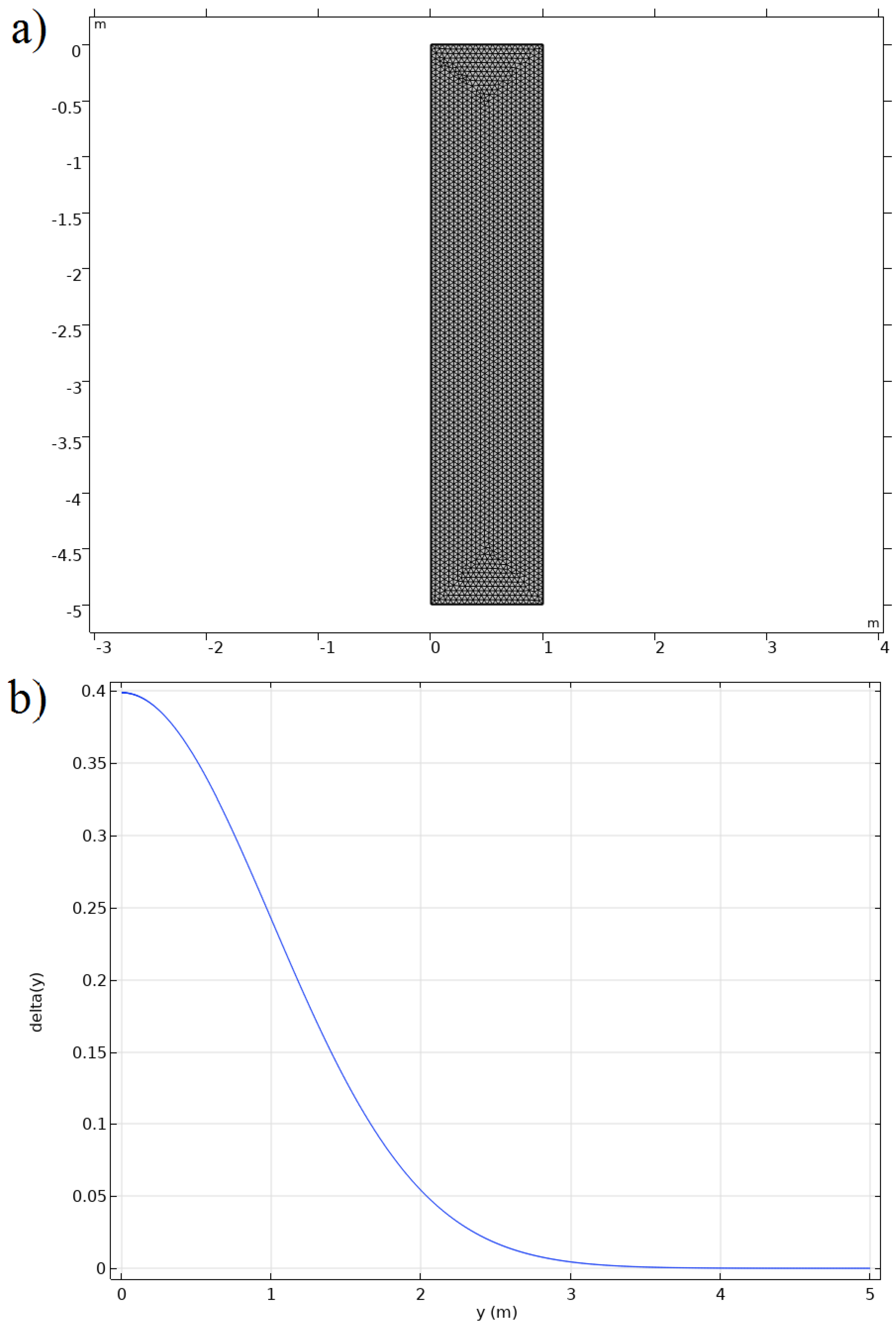
2. Numerical Modelling Using COMSOL Multiphysics

In this section, we developed a model to predict the behaviour of molecular species in a certain fluid, considering the classical partial differential equation (PDE) interface: 2 convection–diffusion in a 2D domain using COMSOL Multiphysics 5.6. COMSOL Multiphysics is one of the most powerful tools used to have a real solution to the PDEs, and the finite element method (FEM) is used to solve the PDE in COMSOL Multiphysics. FEM is the most commonly employed technique for solving problems of engineering and mathematical models, where an approximation of PDEs can be built using different types of discretisations, and then a solution of these PDEs can be obtained numerically [29,30,31]. Table 1 presents the details of generated grids where 5034 triangle elements and 240 elements edge have been created for our geometry.
To simulate Equation (1), we omitted the convection term and the damping coefficient as well since we are focusing here on the time-dependant diffusion coefficient and its effect on the behaviour of the species motion. We defined the diffusion coefficient as a function of time, and we suppose that molecular species start out initially at y = 0 , which means that the initial value describes the injection of molecular species above water layers can be described as u ( y , 0 ) = δ ( y ) , then the concentration will change from an initial delta function to a spread out.
Figure 1a shows the geometry of the reactor and its meshing (5034 triangle elements), where the molecular species are supposed to be transferred in the water reactor (water was chosen as our medium from the builtin materials in COMSOL). Figure 1b shows the initial density profile of the molecular species as a function of distance in the y-axis.

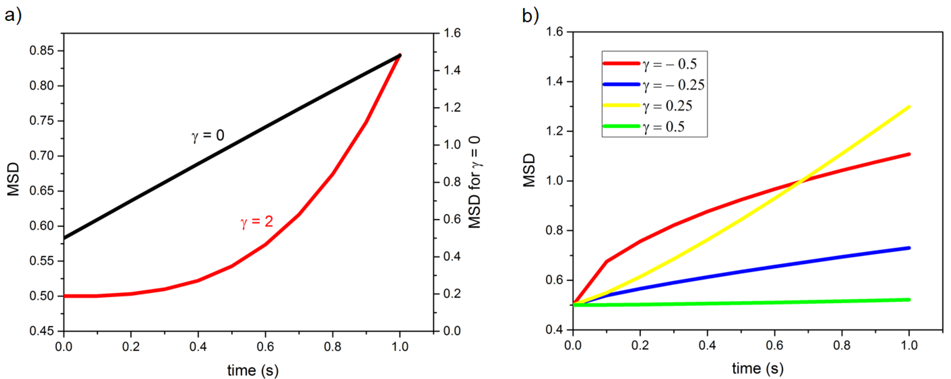
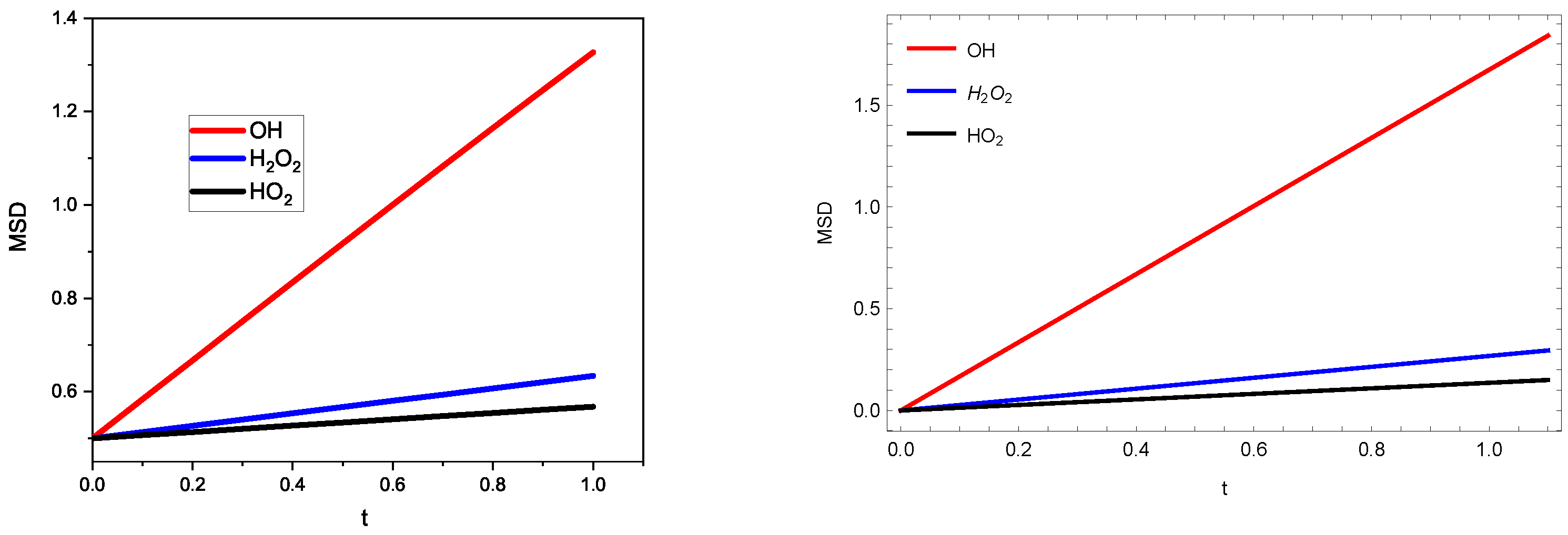
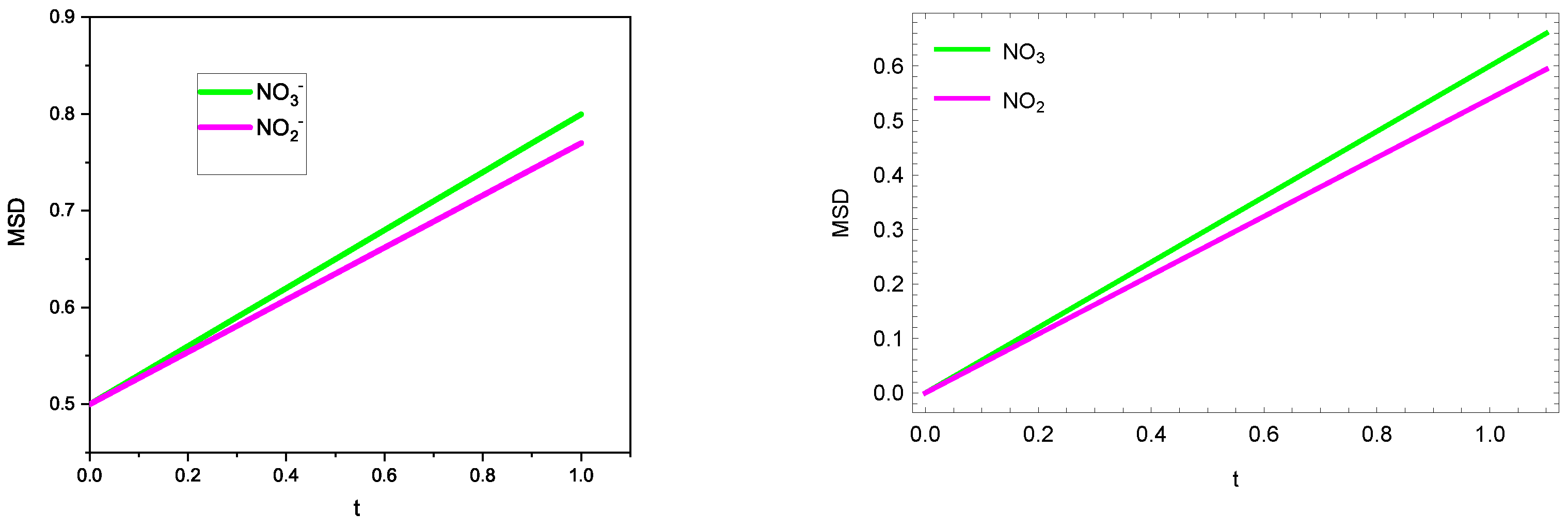
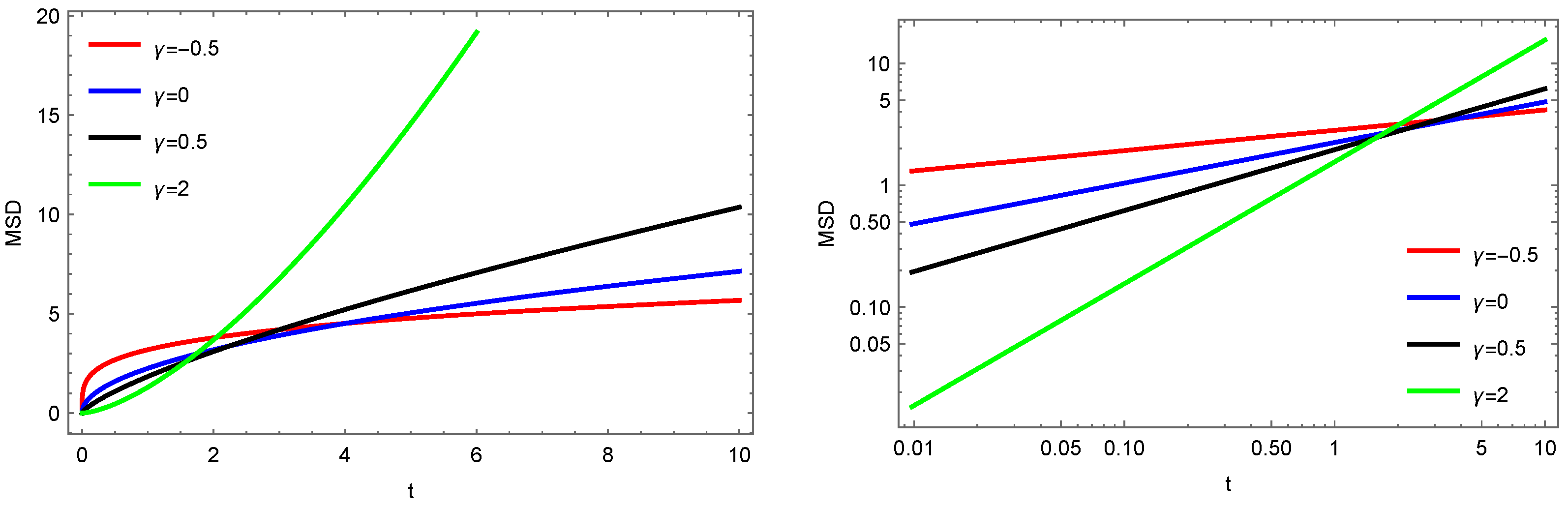
3. Anomalous Diffusion of Molecular Species: Fractional Approach
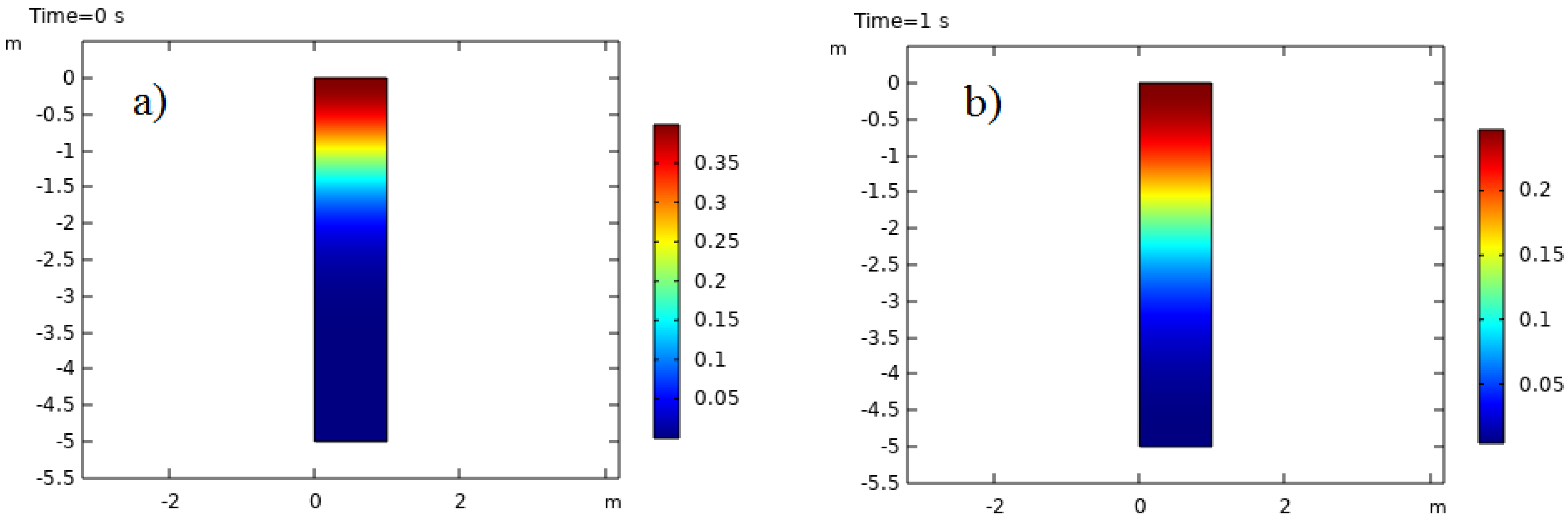
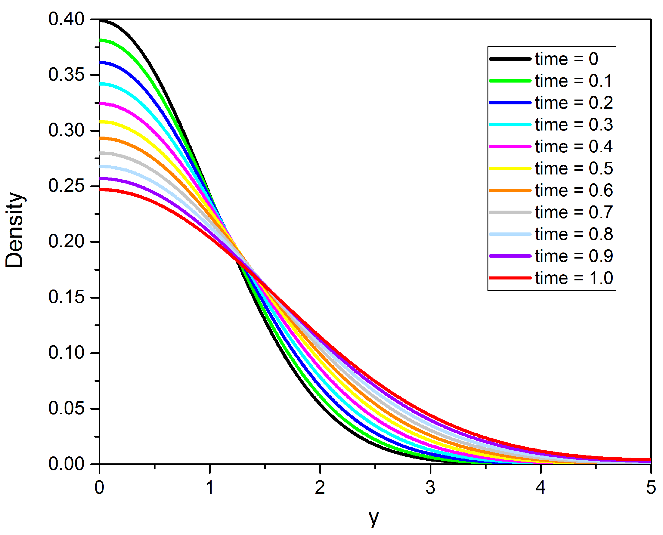
A variety of theoretical techniques have been presented to study non-diffusive transport in complex systems. We focus here on the fractional calculus approach that is widely used to describe anomalous diffusion in order to modulate the diffusive and non-diffusive regimes of different kinds of molecular species. In addition to that, we are interested in comparing our analytical results with numerical simulation results obtained in the previous section so that we can investigate the anomalous mobility by capturing the power-law dependence of the MSD through the fractional-order and the time-dependent diffusion coefficient in one kinetic equation. By generalising the most common form of the diffusion equation with the time-dependent diffusion coefficient, such as suggested by Batchelor and Townsend [32], into the fractional form. Our formalism is based on the regularisation of the so-called Caputo’s fractional derivative to study the dynamical processes of the molecular species in the water layer. We start by considering Equation (1) in the form
1 t γ t α u i ( y , t ) = D γ , α 2 u i ( y , t ) y 2 ,
where the fractional operator in the left hand-side of Equation (2) is representing the Caputo fractional derivative of a function with respect to another function, given by [17,27,28]
1 ϕ ( x ) t β f ( x ) = 1 Γ ( 1 β ) 0 x ϕ ( ξ ) ϕ ( x ) β f ξ d ξ .
The Caputo’s type fractional derivative defined above is considered, for an instant, as a general operator with an arbitrary kernel, which is very useful in overcoming the vast number of the differential operator (see, [27]).
Note that Equation (2) represents one of the contrasting connections between the fractal time process and the fractional Brownian motion, thereby a non-Markovian character with a memory kernel (non-local in time) [33]. Applying a Cosine-Fourier transformation to the Equation (2), then we can obtain
1 t γ t α u i ( k , t ) = D γ , α k 2 u i ( k , t ) .
Consider that u i ( 0 , t ) / y = 0 , and with following the procedure used in [17,28], we obtain
u i ( k , t ) = E α D γ , α t α ( γ + 1 ) ( γ + 1 ) α k 2 ,
where E α is the Mittag-Leffler function, defined as [34]:
E β ( x ) = n = 0 x n Γ ( β n + 1 ) .
Then, we can find the species density u i ( y , t ) via the inverse-Fourier cosine transform of Equation (4) in the following form [17]:
u i ( y , t ) = ( γ + 1 ) α D γ , α t α ( γ + 1 ) M α / 2 ( γ + 1 ) α D γ , α t α ( γ + 1 ) y ,
where, M-Wright function defined as [35]:
M ν ( z ) = k = 0 ( z ) n n ! Γ 1 ν k ν .
Additionally, by using the explicit representations
M 1 / 2 ( z ) = 1 π e z 2 / 4 ,
one can find the solution of Equation (2) in the case of α = 1 , which is given by
u i ( y , t ) = γ + 1 π D γ , α t γ + 1 e γ + 1 4 D γ , α t γ + 1 y 2 .
The above solution is used to describe the fractional Brownian motion with D ( t ) t 2 H 1 in the case of γ + 1 = 2 H , where H indicates the so-called Hurst exponent (for more details see, e.g., [25,36]). Furthermore, in the case of γ = 0 , the solution of Equation (10) is reduced to the familiar solution of the classical diffusion equation (diffusion equation with constant diffusion coefficient), which is given by
u i ( y , t ) = 1 π D γ , α t e y 2 4 D γ , α t .
By having the density of a molecular species, we can calculate the mean square displacement and track the species growth with time from the following identity [23],
y 2 ( t ) = 2 k 2 u i ( k , t ) k = 0 .
Thus, imposing Equation (5) into Equation (12), we obtain an MSD in a general form, such as given in the case of scaled-Brownian motion [37]
y 2 ( t ) = 2 D γ , α t α ( γ + 1 ) ( γ + 1 ) α Γ ( α + 1 ) .
From the Equation (13) (MSD), we can classify the diffusive motion based on the values of fractional order α and the power of diffusion coefficient γ . In the case of 1 < α ( γ + 1 ) < 2 , a super-diffusive process arises, while a sub-diffusive process arises at 0 < α ( γ + 1 ) < 1 and normal diffusion in the case of α ( γ + 1 ) = 1 . Therefore, Equation (13) is a good representative of studying different growing behaviours and crossover among two or more types of diffusive processes. That will not depend only on fractional-order values such as the familiar fractional diffusion equation in the previous case, but on the power parameter of diffusion coefficient ( γ ). Of course, that will be more helpful for tracking the behaviour of different molecular species with different waiting densities and further growth with time inside the water layer, which will be discussed later. Besides that, Equation (13) represents the second moment of the displacement characterising the fractional Brownian motion in the case of α = 1 and γ + 1 = 2 H , such as in [36].

4. Results

In this section, we start by presenting the results of the two parallel models (numerical and analytical), and then the similarity between them will be discussed.
A time-dependent study was performed to simulate Equation (1) to illustrate the change in the density profile of the molecular species in water layers during 1 s using different values of D 0 and γ . Figure 2 shows a colour-coded map of the density propagation through the reactor at (a) time = zero and (b) time = 1 s, where it can be seen that the molecular species travel with time, and its density increases gradually in the reactor. The density profile is shown in Figure 3 for different values of time and γ = 0.25 . It can be seen clearly that density changes with time and decreases significantly at the boundary, while species can travel faster through the reactor. For example, the density decreases more than 60% at the boundary during 1 s, and it can travel deeper in the reactor (approximately 1.5 times) (see the black (for time = 0 s) and the red (for time = 1 s) curves).
To study the normal and anomalous growth of molecular species in a water reactor, the MSD was calculated from the simulation outputs. Figure 4a shows the normal diffusion with γ = 0 , and the linear relation between the MSD and time can be observed clearly (see the black curve and the right y-axis). The superdiffusion can also be seen in Figure 4a (see the red curve and the left y-axis) when using γ = 2 . Moreover, the subdiffusion can be seen for γ = −0.25 and −0.5 (see Figure 4b).
The symmetry between the two models, numerical and analytical, was observed in almost all results. For example, in Figure 3 and Figure 5, the same trends for density profiles were observed, where the density is the maximum at the boundary, and it decreases along the y-axis for each time in both numerical and analytical solutions. However, the density decreases at the boundary with time for both numerical and analytical solutions due to the propagation of the molecular species in the reactor, which results in deep penetration until reaching the end of the reactor dimensions.
Again, the similarity between the results of the two models can be observed when calculating the MSD using different values of γ at α = 1 (see Figure 4 and Figure 6) in which the normal diffusion can be observed at γ = 0 in the illustration of both models. Meanwhile, the super-diffusion can be seen clearly in both models in case of γ > 0 and the sub-diffusion in the case of 1 < γ < 0 , such as: γ = 0.25 and 0.5 .
At the beginning, to test our models, we selected three molecular species OH, H2O2, and HO2 to study their behaviour in water layers and compare it to the results of MD simulation published before [11], where we used the following diffusion coefficients: 0.837, 0.134, and 0.068 Å 2 /ps for OH, H2O2, and HO2, respectively, that were used in the mentioned work. The numerical and analytical were solved using these values, and consequently, we calculated the MSD (see Figure 7). As it can be seen clearly from Figure 7, the diffusivity of the H2O2 molecule is in between OH and HO2, and these results correspond well with the published data using the MD simulation [11]. Moreover, to test the validity of our models for other molecular species, we chose two more species (for their importance in plasma medicine): nitrite (NO3-) and nitrate (NO2-); they are common nitrogen oxyanions that constitute the basic forms of nitric (HNO3) and nitrous (HNO2) acids. To calculate MSD for NO3- and NO2-, we used the diffusion coefficients in a recently published MD simulation results as 0.3 and 0.27Å 2 /ps, respectively [38]. The MSD using both models can be seen clearly in Figure 8. However, though the values of diffusion coefficients for NO3- and NO2- are very close to each other, our models were able to distinguish between their MSD, as can be seen from Figure 8; a high similarity can also be observed between the numerical and analytical models.
Finally, in Figure 9, we show the MSDs for different values of the power-law time-dependent diffusion coefficient at α = 1 / 2 . From that figure, it can be shown that decreasing the value of γ decreases the rate of diffusivity. That means the power-law index ( γ ) with the time-fractional order ( α ) plays an essential role in illustrating the MSD at a short and long timescale, based on the value of α ( γ + 1 ) , which controls the type of diffusivity according to Figure 4, Figure 6 and Figure 9. Consequently, the value of α ( γ + 1 ) determines the type of diffusion (sub, normal, or superdiffusion) instead of the value of time-fractional order α . In general, Equation (13) allows us to describe superdiffusion in coordinate space, which may be surprising, as time-fractional derivatives are usually associated with subdiffusion.

5. Conclusions and Future Work

In many physical scenarios, molecular species may diffuse in different manners inside liquid layers. For instance, in a short time, a species can exhibit a slow diffusion, and over time, the species’ motion crosses to normal or fast diffusion. Thus, the time-fractional diffusion equation with the power-law time-dependent diffusion coefficient is a good representative method to track the behaviour of molecular species over time. In this respect, the density profiles for different molecular species with the mean square displacement were studied numerically via COMSOL Multiphysics and analytically via the fractional approach. Our model is based on the general solution of standard and fractional diffusion equations with time-dependent diffusivity. Moreover, these findings can help us to understand the different transport regimes of ROS with biological targets, especially those that occurred in a very short time. Our analysis here just discusses the similarity between the numerical simulation and the fractional kinetic model under the assumption of a time-dependent diffusion coefficient. This is considered as a preface to compare our model with an experimental study tracking the density of molecular species in liquid layers. Moreover, development of our model to study the permeability of molecular species through biological media is one of our main targets in future work.

Author Contributions

Conceptualization, M.M.H. and A.M.T.; Data curation, M.M.H. and A.M.T.; Formal analysis, M.M.H. and A.M.T.; Investigation, M.M.H. and A.M.T.; Methodology, M.M.H. and A.M.T.; Writing—original draft, M.M.H. and A.M.T.; Writing—review and editing, M.M.H. and A.M.T. All authors have read and agreed to the published version of the manuscript.

Funding

This research was funded by Future University in Egypt, Cairo 11835, Egypt.

Institutional Review Board Statement

Not applicable.

Informed Consent Statement

Not applicable.

Data Availability Statement

Not applicable.

Conflicts of Interest

The authors declare no conflict of interest.

References

  1. Laroussi, M. Plasma medicine: A brief introduction. Plasma 2018, 1, 5. [Google Scholar] [CrossRef] [Green Version]
  2. Fridman, G.; Friedman, G.; Gutsol, A.; Shekhter, A.B.; Vasilets, V.N.; Fridman, A. Applied plasma medicine. Plasma Process. Polym. 2008, 5, 503–533. [Google Scholar] [CrossRef]
  3. Adamovich, I.; Baalrud, S.; Bogaerts, A.; Bruggeman, P.; Cappelli, M.; Colombo, V.; Czarnetzki, U.; Ebert, U.; Eden, J.; Favia, P.; et al. The 2017 Plasma Roadmap: Low temperature plasma science and technology. J. Phys. D Appl. Phys. 2017, 50, 323001. [Google Scholar] [CrossRef]
  4. Samukawa, S.; Hori, M.; Rauf, S.; Tachibana, K.; Bruggeman, P.; Kroesen, G.; Whitehead, J.C.; Murphy, A.B.; Gutsol, A.F.; Starikovskaia, S.; et al. The 2012 plasma roadmap. J. Phys. D Appl. Phys. 2012, 45, 253001. [Google Scholar] [CrossRef]
  5. Yokoyama, T.; Kogoma, M.; Kanazawa, S.; Moriwaki, T.; Okazaki, S. The improvement of the atmospheric-pressure glow plasma method and the deposition of organic films. J. Phys. D Appl. Phys. 1990, 23, 374. [Google Scholar] [CrossRef]
  6. Fridman, A. Plasma Chemistry; Cambridge University Press: Cambridge, UK, 2008. [Google Scholar]
  7. El-Kalliny, A.S.; Abd-Elmaksoud, S.; El-Liethy, M.A.; Abu Hashish, H.M.; Abdel-Wahed, M.S.; Hefny, M.M.; Hamza, I.A. Efficacy of Cold Atmospheric Plasma Treatment on Chemical and Microbial Pollutants in Water. ChemistrySelect 2021, 6, 3409–3416. [Google Scholar] [CrossRef]
  8. Hefny, M.M.; Nečas, D.; Zajíčková, L.; Benedikt, J. The transport and surface reactivity of O atoms during the atmospheric plasma etching of hydrogenated amorphous carbon films. Plasma Sources Sci. Technol. 2019, 28, 035010. [Google Scholar] [CrossRef]
  9. Kaushik, N.K.; Kaushik, N.; Linh, N.N.; Ghimire, B.; Pengkit, A.; Sornsakdanuphap, J.; Lee, S.J.; Choi, E.H. Plasma and nanomaterials: Fabrication and biomedical applications. Nanomaterials 2019, 9, 98. [Google Scholar] [CrossRef] [Green Version]
  10. Benedikt, J.; Hefny, M.M.; Shaw, A.; Buckley, B.; Iza, F.; Schäkermann, S.; Bandow, J. The fate of plasma-generated oxygen atoms in aqueous solutions: Non-equilibrium atmospheric pressure plasmas as an efficient source of atomic O (aq). Phys. Chem. Chem. Phys. 2018, 20, 12037–12042. [Google Scholar] [CrossRef] [Green Version]
  11. Yusupov, M.; Neyts, E.; Simon, P.; Berdiyorov, G.; Snoeckx, R.; Van Duin, A.; Bogaerts, A. Reactive molecular dynamics simulations of oxygen species in a liquid water layer of interest for plasma medicine. J. Phys. D Appl. Phys. 2013, 47, 025205. [Google Scholar] [CrossRef] [Green Version]
  12. Bogaerts, A.; Yusupov, M.; Razzokov, J.; Van der Paal, J. Plasma for cancer treatment: How can RONS penetrate through the cell membrane? Answers from computer modeling. Front. Chem. Sci. Eng. 2019, 13, 253–263. [Google Scholar] [CrossRef]
  13. Amhamed, A.; Atilhan, M.; Berdiyorov, G. Permeabilities of CO2, H2S and CH4 through choline-based ionic liquids: Atomistic-scale simulations. Molecules 2019, 24, 2014. [Google Scholar] [CrossRef] [PubMed] [Green Version]
  14. Rais, D.; Menšik, M.; Paruzel, B.; Toman, P.; Pfleger, J. Concept of the time-dependent diffusion coefficient of polarons in organic semiconductors and its determination from time-resolved spectroscopy. J. Phys. Chem. C 2018, 122, 22876–22883. [Google Scholar] [CrossRef]
  15. Cherstvy, A.G.; Safdari, H.; Metzler, R. Anomalous diffusion, nonergodicity, and ageing for exponentially and logarithmically time-dependent diffusivity: Striking differences for massive versus massless particles. J. Phys. D Appl. Phys. 2021, 54, 195401. [Google Scholar] [CrossRef]
  16. Crank, J. The Mathematics of Diffusion; Oxford University Press: Oxford, UK, 1979. [Google Scholar]
  17. Garra, R.; Giusti, A.; Mainardi, F. The fractional Dodson diffusion equation: A new approach. Ric. Mat. 2018, 67, 899–909. [Google Scholar] [CrossRef] [Green Version]
  18. Tawfik, A.M.; Hefny, M.M. Subdiffusive Reaction Model of Molecular Species in Liquid Layers: Fractional Reaction-Telegraph Approach. Fractal Fract. 2021, 5, 51. [Google Scholar] [CrossRef]
  19. Hefny, M.M.; Pattyn, C.; Lukes, P.; Benedikt, J. Atmospheric plasma generates oxygen atoms as oxidizing species in aqueous solutions. J. Phys. D Appl. Phys. 2016, 49, 404002. [Google Scholar] [CrossRef]
  20. Batchelor, G. Diffusion in a field of homogeneous turbulence: II. The relative motion of particles. In Mathematical Proceedings of the Cambridge Philosophical Society; Cambridge University Press: Cambridge, UK, 1952; Volume 48, pp. 345–362. [Google Scholar]
  21. Nagy, Á.; Omle, I.; Kareem, H.; Kovács, E.; Barna, I.F.; Bognar, G. Stable, Explicit, Leapfrog-Hopscotch Algorithms for the Diffusion Equation. Computation 2021, 9, 92. [Google Scholar] [CrossRef]
  22. Metzler, R.; Klafter, J. From a generalized chapman- kolmogorov equation to the fractional klein- kramers equation. J. Phys. Chem. B 2000, 104, 3851–3857. [Google Scholar] [CrossRef]
  23. Metzler, R.; Klafter, J. The random walk’s guide to anomalous diffusion: A fractional dynamics approach. Phys. Rep. 2000, 339, 1–77. [Google Scholar] [CrossRef]
  24. Evangelista, L.R.; Lenzi, E.K. Fractional Diffusion Equations and Anomalous Diffusion; Cambridge University Press: Cambridge, UK, 2018. [Google Scholar]
  25. Bologna, M.; Svenkeson, A.; West, B.J.; Grigolini, P. Diffusion in heterogeneous media: An iterative scheme for finding approximate solutions to fractional differential equations with time-dependent coefficients. J. Comput. Phys. 2015, 293, 297–311. [Google Scholar] [CrossRef]
  26. Fa, K.S.; Lenzi, E. Time-fractional diffusion equation with time dependent diffusion coefficient. Phys. Rev. E 2005, 72, 011107. [Google Scholar] [CrossRef] [PubMed]
  27. Almeida, R. A Caputo fractional derivative of a function with respect to another function. Commun. Nonlinear Sci. Numer. Simul. 2017, 44, 460–481. [Google Scholar] [CrossRef] [Green Version]
  28. Tawfik, A.M.; Abdelhamid, H.M. Generalized fractional diffusion equation with arbitrary time varying diffusivity. Appl. Math. Comput. 2021, 410, 126449. [Google Scholar] [CrossRef]
  29. Rabanimehr, F.; Farhadian, M.; Solaimany Nazar, A.R.; Behineh, E.S. Simulation of photocatalytic degradation of methylene blue in planar microreactor with integrated ZnO nanowires. J. Appl. Res. Water Wastewater 2021, 8, 36–40. [Google Scholar]
  30. Janczarek, M.; Kowalska, E. Computer simulations of photocatalytic reactors. Catalysts 2021, 11, 198. [Google Scholar] [CrossRef]
  31. Hasanpour, M.; Motahari, S.; Jing, D.; Hatami, M. Numerical modeling for the photocatalytic degradation of methyl orange from aqueous solution using cellulose/zinc oxide hybrid aerogel: Comparison with experimental data. Top. Catal. 2021, 1–14. [Google Scholar] [CrossRef]
  32. Klafter, J.; Silbey, R. Derivation of the continuous-time random-walk equation. Phys. Rev. Lett. 1980, 44, 55. [Google Scholar] [CrossRef] [Green Version]
  33. Lutz, E. Fractional langevin equation. In Fractional Dynamics: Recent Advances; World Scientific: Singapore, 2012; pp. 285–305. [Google Scholar]
  34. Gorenflo, R.; Kilbas, A.A.; Mainardi, F.; Rogosin, S.V. Mittag-Leffler Functions, Related Topics and Applications; Springer: Berlin/Heidelberg, Germany, 2014. [Google Scholar]
  35. Mainardi, F.; Pagnini, G. The Wright functions as solutions of the time-fractional diffusion equation. Appl. Math. Comput. 2003, 141, 51–62. [Google Scholar] [CrossRef] [Green Version]
  36. Wang, K.; Lung, C. Long-time correlation effects and fractal Brownian motion. Phys. Lett. A 1990, 151, 119–121. [Google Scholar] [CrossRef]
  37. Wang, W.; Cherstvy, A.G.; Liu, X.; Metzler, R. Anomalous diffusion and nonergodicity for heterogeneous diffusion processes with fractional Gaussian noise. Phys. Rev. E 2020, 102, 012146. [Google Scholar] [CrossRef] [PubMed]
  38. Cordeiro, R.M.; Yusupov, M.; Razzokov, J.; Bogaerts, A. Parametrization and molecular dynamics simulations of nitrogen oxyanions and oxyacids for applications in atmospheric and biomolecular sciences. J. Phys. Chem. B 2020, 124, 1082–1089. [Google Scholar] [CrossRef] [PubMed]
Figure 1. (a) Model geometry presents the extremely fine mesh for water reactor, and (b) the initial density profile using Dirac delta function.
Symmetry 14 01146 g001
Figure 2. A 2D colour-coded map represents the propagation of molecular species in water layers at (a) time = 0 s and (b) time = 1 s.
Symmetry 14 01146 g002
Figure 3. Density profiles of molecular species through y-axis for different times at γ = 0.25 using the numerical method.
Symmetry 14 01146 g003
Figure 4. MSD using the numerical method for different values of γ .
Symmetry 14 01146 g004
Figure 5. Density profiles of molecular species for different times at γ = 0.25 and α = 1 using the analytical method.
Symmetry 14 01146 g005
Figure 6. MSD using the analytical method for different values of γ in the case of α = 1 .
Symmetry 14 01146 g006
Figure 7. MSD for the selected molecular species: OH, H2O2, and HO2 using the numerical method (left panel) and analytical method (right panel).
Symmetry 14 01146 g007
Figure 8. MSD for NO3- and NO2- using the numerical method (left panel) and analytical method (right panel).
Symmetry 14 01146 g008
Figure 9. MSD for different values of γ in the case of α = 1 / 2 (left panel) with the double logarithmic plot (right panel).
Symmetry 14 01146 g009
Table 1. Element statistics of the used mesh in our numerical model.
Element TypeNumber
Triangles5034
Edge elements240
Vertex element4
Number of elements5034
Element area ratio0.3717
Mesh area5 m 2
Average element quality0.9457
Publisher’s Note: MDPI stays neutral with regard to jurisdictional claims in published maps and institutional affiliations.

