Abstract
To solve the energy efficiency (EE) optimization in a multi-cell (MU) massive multiple-input multiple-output (MIMO) downlink system, of which channels are of symmetry in the Time-Division Duplex (TDD) protocol, we utilize a spatially correlated channel model and adopt the minimum mean-squared error (MMSE) estimator to tailor linear precoding vectors. Then, we derive the expression of downlink spectral efficiency (SE), taking interference into account. Subsequently, we establish the EE optimization function, which is defined as the average capacity divided by power consumption. In an interference-limited scenario, the EE optimization is of high complexity to solve globally as it is not jointly concave. To this end, we propose the Dinkelbach-like power allocation algorithm to obtain a suboptimal solution. We transform the EE problem in a fractional form into a subtractive optimization form called an auxiliary subproblem. Then, we relax the sub-problem to a concave problem by initializing the interference and omitting the dynamic power term about throughput. Lastly, we solve iteratively the Karush–Kuhn–Tucker (KKT) conditions by bisection search. Consequently, we obtain a sub-solution with modest complexity. The simulation results justify the rationality of the Dinkelbach-like algorithm and demonstrate that the proposal outperforms the reference schemes and effectively improves the performance metrics EE and SE.
1. Introduction
Concerning the vision of ubiquitous wireless intelligence, emerging Internet of Everything applications will require a convergence of communication, sensing, control, and computing functionalities [1]. Many widely anticipated future services, including eHealth and autonomous vehicles, will be critically dependent on the delivery of high reliability and low latency with high data rates, which consequently calls for a higher area throughput and delivering must-have services due to the imminent data traffic crunch and the rising expectations of service quality. Moreover, the amount of data traffic growing at an exponential pace entails not only a dramatic improvement in spectral efficiency (SE) but also steep power consumption. Consequently, both economic and environmental concerns are in compelling need of consideration in addition to the demand for data traffic [2]. To this end, energy efficiency emerges as SE is unable to characterize an energy-efficient network, which is highlighted in next-generation network designs. Notably, massive multiple-input multiple-output (MIMO) stands out in various candidate technologies as providing significant improvements in spectral efficiency and energy efficiency, which enables a set of user equipment (UE) to serve over the same time–frequency interval by deploying multiple receive antennas [3]. Hence, energy efficiency optimization in massive MIMO has received tremendous attention.
Spurred by both economic and environmental concerns, energy efficiency (EE) has been exposed to extensive research to satisfy the energy-efficient performance metric vital to the sixth-generation communication network. Academic researchers have spared no effort to seek seminal contributions to improving energy-efficient performance, such as resource allocation, energy harvesting, and network deployment [2]. Herein, we cast our attention to power allocation as maximizing the energy efficiency with a given transmit power budget in line with not increasing energy consumption. The study [4] considered the maximization of the global energy efficiency, as well as of the minimum energy efficiency, which is nonconvex. Exploiting the fractional programming and sequential convex develops a power allocation algorithm that guarantees the convergence to a Karush–Kuhn–Tucker (KKT) point. However, it comes at the cost of high computational complexity and feedback requirements. In the study [5], EE optimization in the downlink multi-cell massive MIMO was investigated, which took into account different users’ quality-of-service requirements. An iterative optimization algorithm was obtained by alternating optimization about the optimal amount of data rate, the number of antennas, and users. Thus, it was of high complexity incurred from the alternating iterations of multiple parameters. The study [6] proposed an adaptive power allocation to maximize the SE and EE in a MIMO broadcast channel. Applying the Lagrangian method solved the objective function, which involved a threshold of the effective capacity for each user. However, both [5,6] apply to the special case of spatially uncorrelated fading channels with perfect channel state information (CSI). The study [7] used an energy-efficient low-complexity algorithm (EELCA) to obtain an optimal power allocation solution based on Newton’s methods in the noise-limited scenario, and it exploited the linear power allocation and perfect CSI. In fact, it is challenging to acquire perfect CSI due to the presence of the channel estimation error. The studies [8,9] proposed power allocation for an energy-efficient massive MIMO with imperfect CSI, while the power consumption models were linear about antennas and UE. The study [10] investigated energy efficiency and the spectral efficiency trade-off for a single-cell massive MIMO downlink transmission with statistical channel state information available at the transmitter. A low-complexity suboptimal two-layer water-filling-structured power allocation algorithm was proposed, which reached near-optimal performance. Practical channels were generally spatially correlated, also known as having space-selective fading [11]. In the study [12], to address the EE optimization in a multi-cell downlink massive MIMO operating over spatially correlated Rician fading channels with imperfect CSI, the authors transformed the problem into a geometric program and developed an iterative power allocation algorithm under the constraints of a given sum spectral efficiency and a maximum total. Nevertheless, the closed-form solution came at the expense of staggering computational complexity.
From the above analysis, extensive studies have been conducted on EE optimization in massive MIMO with perfect CSI, whereas the case with imperfect CSI in an interference-limited scenario is still open to be studied due to its nonconvexity. In addition, the linear power allocation model taking users and antennas into account has been widely used, which is adopted in studies [13,14,15], for instance. Consequently, we consider spatially correlated Rayleigh fading channels with imperfect CSI and exploit the nonlinear power consumption model, which encompasses dynamic power about throughput and nonlinear power terms from BS’s computation in contrast to the linear power model. The global optimum acquisition comes at the price of unbearable computational complexity as the objective is tough to convert to a convex problem. Herein, we propose a computationally efficient power allocation scheme called Dinkelbach-like power allocation to obtain a suboptimal solution with limited complexity, and the simulation results manifest that the proposed power allocation is a computationally efficient method that jointly increases EE and SE and, meanwhile, performs well in SE fairness compared to several reference schemes.
The remainder of this paper is organized as follows: The spatially correlated channel model is described and spectral efficiency is derived by adopting the minimum mean-squared error (MMSE) estimator and maximum ratio (MR) precoding in Section 2. In Section 3, a realistic power consumption model is considered and the EE optimization of multi-cell multi-user massive MIMO is obtained. Subsequently, Section 4 proposes a sub-optimal power allocation algorithm. In the last section, the simulation results and conclusion are presented.
Notation: In this paper, matrices and column vectors are denoted by upper-case bold letters and lower-case bold letters, respectively; and denote the conjugate transpose and the complex conjugate of matrix A, respectively, and is the transpose; denotes a unit matrix of order M; denotes the Euclidean norm of a scalar, and denotes the mathematical expectation. denotes the (j, k)th element of a matrix .
2. System Model
Provided spatially correlated channels in the non-line-of-sight case are considered, also referred to as having space-selective fading, a more general and realistic model is generated by the local scattering spatial correlation model. In addition, each coherence block is operated in Time-Division Duplex (TDD) mode for the sake of saving for pilots’ overhead, as a result of downlink channels symmetrical to uplink counterparts.
2.1. Channel Model
Suppose each cell of L cells covers a square, where each base station (BS) equipped with M antennas located in the center of the corresponding cell serves K single-antennas, and user equipment (UE) drops uniformly at distances larger than 35 m from the serving BS to guarantee a plane wave reaches it. The multi-cell massive MIMO downlink model is illustrated in Figure 1.
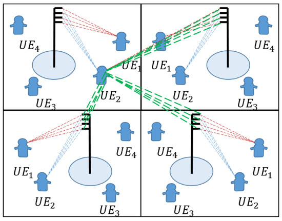
Figure 1.
Illustration of the downlink massive MIMO model.
As the spatially correlated channel model is regarded as Rayleigh fading, it is essential to generate a channel response vector as .
Notice that the subscript indicates the identity of the kth UE in cell j, while the superscript is the index of the serving BS l. Due to the scattering, the received signal is the superposition of N multipath components, illustrated in Figure 2, where accounts for the gain and phase-rotation for the nth path, which implicitly implies the relevance to spatial correlation and large-scale gain. is antenna spacing, which is measured in the number of wavelengths between adjacent antennas. , where is a deterministic nominal angle once given a drop and is a random deviation from the .
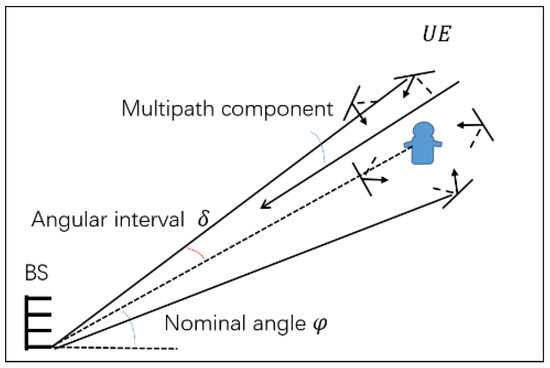
Figure 2.
Illustration of non-line-of-sight propagation under the local scattering model.
The multidimensional central limit theorem then implies convergence. Subsequently, it follows from the th element of the spatial correlation matrix that
Spatial correlation is the function with respect to angular distribution. and the average channel gain “ is denoted by
where determines the median channel gain at a reference distance of 1 km and path-loss exponent determines how fast the signal decays. is called shadow fading. is the distance of to its serving BS j. The variance R is interpreted as the macroscopic large-scale fading, which includes distance-dependent path loss, shadowing, antenna gains, and penetration losses in non-line-of-sight propagation.
2.2. Channel Estimation and Linear Processing
MIMO brings a coextensive increase in intercell and intracell interference due to space-division multiple access. To make efficient use of the Massive MIMO, each BS needs to estimate the channel responses to perform interference suppression. As the TDD protocol illustrated in Figure 3 is matched to the coherence blocks, the uplink and downlink channels are considered reciprocal and symmetrical [16], and the BS can make use of uplink estimates for both reception and downlink transmission.
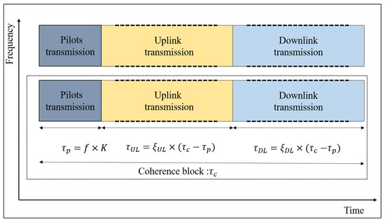
Figure 3.
Illustration of the TDD protocol.
As we assume, samples are reserved for uplink pilot transmission in each coherence block. The pilot sequence of is denoted by , which satisfies . After uplink pilot transmission, the BS received uplink signal is given by
where is the additive white-Gaussian-noise-distributed ,and is the uplink pilot transmit power. To estimate a particular UE, multiplying the received signal with its pilot sequence obtains the corresponding received pilot signal given as
Using a pilot book with mutually orthogonal sequences, the MMSE estimate of the uplink channel is denoted by [17]
where , means utilizes the same pilot sequences as , and is the pilot sequence assigned to .
The precoding design typically strikes a tradeoff between eliminating the intercell interference and maximizing the signal-to-interference-to-noise ratio (SINR). A simple and popular one is the maximum ratio (MR) precoding scheme. As uplink channels and downlink channels are symmetrical, the BS can conveniently use uplink estimates to tailor the precoding vectors in the downlink. The expression is
where the precoding vector is tailored for UE k in cell j, namely , which determines the spatial directivity of the transmission.
2.3. Downlink Spectral Efficiency
Each BS transmits payload data to its UEs in the downlink (DL), using MR linear precoding. denotes the random data signal intended for , namely UE k in cell j, for j = 1, …, L and k = 1, …, K. The desired signal to UE k in cell j propagates over the precoded channel , where is tailored for UE k in cell j. UE can blindly obtain the scalar of from the payload data signals. The signal power is the transmit power allocated to this UE. The UE does not know the precoded channel a priori but can approximate it with the mean value , which is a reasonable assumption due to channel hardening [18]. Therefore, the received DL signal can be expressed as
where is independent addictive receiver noise with variance . As the average precoded channel is deterministic, and the remaining terms are uncorrelated with the signal , then the DL ergodic channel capacity of UE k in cell j can be lower-bounded as
Equation (9) is referred to as the use-and-then-forget (UatF) bound as the channel estimates are used for precoding and not for signal detection [19]. For simplicity, (9) can be expressed more compactly as
For UE k in cell j, where (12) and (13) are the average channel gain and average interference gain, respectively,
where signal power is the transmit power allocated to , is the sample numbers per coherence block, and is the sample numbers for downlink transmission. In addition, all other coefficients are positive parameters that do not depend on the . Given the fact that multi-user interference is present, the is expressed according to the concave fractional signal-to-interference-plus-noise ratio (SINR) in the useful power, which is coupled, that is, each UE’s SINR depends on all UEs’ transmit power.
3. Power Consumption Model and Energy Efficiency
The EE of a cellular network is the number of bits that can be reliably transmitted per unit of energy [17]. Energy efficiency is the ratio of throughput and energy consumption.
3.1. Power Consumption Model
Tractable but less realistic models may instead reach a misleading conclusion about EE [20]. Herein, we introduce a power consumption model that quantifies the circuit power incurred by signal processing, backhaul signaling, encoding, and decoding. It can be quantified as
where and are the power amplifier efficiencies of UE and BS, respectively, and is the power for uplink (UL) pilot transmission. For more details, please refer to the monograph [17], for the sake of space constraints. Notice that the power model is derived concerning the MMSE estimator and MR signal schemes adopted. The parameters are explained in the simulation parameter setting.
3.2. Downlink Energy Efficiency
Global energy efficiency (GEE) as the optimization objective we adopt herein, which sticks to the physical meaning of energy efficiency, is a ratio of throughput and energy consumption. The GEE optimization follows from substantial insight into the above. Subsequently, we put forward the optimization problem, which is mathematically formulated as:
P is the set of all feasible transmit power solutions that satisfy the given constraints on the BS of each cell, where refers to the optimization variable. Before delving into the EE analysis, from intuition, it can be grasped that the numerator is not jointly concave in , nor for the denominator, which means it requires exponential complexity or is even more intractable. For analytical simplicity, we tackle energy-efficient power allocation optimization by keeping the M fixed. As we have observed, no computationally efficient algorithm exists to solve a problem that is not jointly concave in , where . To date, determining the global solutions of energy-efficient power allocation in interference-limited scenarios is still an open problem. There is a performance–complexity tradeoff from the analysis above. It is tricky to obtain a global optimum dealing with a generic optimization.
4. Dinkelbach-Like Power Allocation
In what follows, we propose a suboptimal algorithm based on Dinkelbach’s algorithm called the Dinkelbach-like algorithm to optimize EE in the setup scenario with lower computational complexity. As we can see, the optimization problem belongs to nonconcave programming problems and requires high computational complexity to obtain an optimum. Motivated by Dinkelbach’s algorithm, we transform the EE problem in a fractional form into a subtractive optimization form called the auxiliary sub-problem employing Dinkelbach’s algorithm. To solve globally the auxiliary sub-problem given a parameter in each iteration of Dinkelbach’s algorithm entails unaffordable complexity as it is not a concave problem, which prevents the application of the formal Dinkelbach’s algorithm. To this end, we relax the sub-problem to a concave problem by initializing the interference and omitting the dynamic power term about throughput, subsequently iteratively solving the KKT conditions by bisection search.
4.1. Transformation of EE Optimization Problem
Dinkelbach’s algorithm belongs to the class of parametric algorithms [21], whose basic idea is to tackle a concave-convex fractional problem (CCFP) by solving a sequence of easier problems that converges to the global solution of the CCFP [22]. Unfortunately, the objective of the EE optimization problem is a generic fractional problem instead. Similarly, we transform the EE optimization problem via Dinkelbach’s algorithm, expressed as
Then, the global optimum can be obtained using Algorithm 1. Unfortunately, the maximization of the sub-problem is solved globally at the price of high computational complexity, even more impossible to solve. It is critical to tackle the sub-problem properly with affordable complexity.
| Algorithm 1. Dinkelbach’s algorithm |
| Input |
| Output |
| 1: whiledo |
| 6: end while |
4.2. Solution of Auxiliary Sub-Problem
As we can see, Dinkelbach’s algorithm requires solving globally the auxiliary sub-problem in step 2 given a parameter value. Herein, we obtain an auxiliary sub-problem expressed as
As aforementioned, the first term of the objective is non-jointly concave in , so the second is also naturally nonconcave due to the presence of , which means it does not enjoy the convexity that enables solving globally with limited complexity. Hence, we propose a low-complexity algorithm at the price of obtaining a sub-optimum of (17) called the primal auxiliary sub-problem. The concave approximation is obtained after specific pretreatment to (17), and then we can iteratively solve the KKT conditions of the former globally. As a consequence, the global optimum guarantees the convergence of the proposed algorithm and is an approximate solution to (17).
4.2.1. Initialization of the Sub-Problem
The difficulty lies in the fact that the first term is not jointly concave, due to the presence of interference and the second term couples the first term. To this end, an approximation more tractable can be obtained through initializing the SINR-like term in equal power allocation, given by
After specific pretreatment, is
Considering the multi-cell MIMO system is symmetric, we decompose the coupled L cells into L individual cells as each link depends only on the transmit power of its own cell after the initialization operation. In the meanwhile, the power consumption omits the dynamic counterpart related to , which is a valid approximation followed by neglecting small terms as explained in the next section. It can be observed that a concave problem holds provided the nonnegativity of , which is ensured due to the nonnegativity of the numerator and the positivity of the denominator.
4.2.2. Acquisition of KKT Conditions
The global optimum follows from the convexity’s optimality condition, which guarantees the convergence of the Dinkelbach-like algorithm. If and only if each auxiliary sub-problem is solved globally, the generalized Dinkelbach’s algorithm converges to the global solution of the fractional problem [21]. Herein, (18) could be solved globally utilizing any convex programming algorithm. Denoting the Lagrange multipliers for constraints by and , the Lagrangian function of (15) is written as
In addition, the KKT conditions of (18) are expressed as
where (21a) is the Lagrangian stationarity conditions, (21b) is the nonnegativity of the multipliers, (21c) and (21d) are the problem constraints, while (21e) is the complementary slackness condition. Any solution of (21) is also a global solution of (17) given its convexity. To solve the KKT system (21) directly is difficult, so an iterative algorithm can be developed by starting from a feasible transmit power vector and iteratively updating the transmit powers by (22), the updating equation, given by
This can be efficiently solved by Algorithm 2 on the multiplier . The resulting formal procedure can be stated as follows:
| Algorithm 2. Bisection for sub-problem |
| Input: Pmax itermax |
| Output: |
| 1: Initialize: compute according to equation (22) |
| 2: while Pmax do |
| 3: compute according to equation (22) |
| 4: end while |
| 5: compute according to equation (22) |
| 6: while Pmax + || Pmax + do |
| 7: if iter > itermax then |
| 8: break |
| 9: end if |
| 10: if Pmax then |
| 11: |
| 12: else |
| 13: |
| 14: end if |
| 15:; compute according to equation (22); iter iter + 1 |
| 16: end while |
| 17: return |
4.3. Iteration of the Parameter
In the end, we generalize Dinkelbach’s algorithm to obtain a suboptimum of the original EE optimization (15) with affordable complexity after approximating the sub-problem. The Dinkelbach-like algorithm can be stated as in Algorithm 3.
| Algorithm 3. Dinkelbach-like algorithm for power allocation |
| Input: |
| Output: |
| 1: initialize: |
| 2: while do |
| 3: solve the sub-problem according to algorithm 2 |
| 4: |
| 5: |
| 6: |
| 7: end while |
5. Simulation Results and Discussion
To exemplify the performance metrics of a symmetric multi-cell massive MIMO system composed of four square cells, the system parameters of Monte Carlo simulations are detailed below in Table 1. MATLAB R2018b is used for simulation. Unless otherwise specified, we use the Value set 1 by default for simulations. To verify the rationality and superiority of the algorithm proposed in this paper, several classical power distribution algorithms are selected as references for comparison. The max-min fairness scheme makes UE operate at the same SE level, which sacrifices a certain spectrum efficiency in exchange for maximum user fairness, as a user fairness benchmark. The maximum product SINR algorithm denoting maxprod based on the interior point method aims at maximizing the product of the SINR.

Table 1.
System parameters of the simulation setup.
5.1. Simulation Parameters
5.2. Analysis of Simulation Results
To illustrate the power consumption model impact on EE, four widely used power models are compared including model 1 [10], model 2 [9], model 3 [23], and model 4 we adopt. As model 1 only takes radio frequency (RF) chains into account, model 2 includes the power consumption of UEs. The difference between model 3 and model 2 is the presence of dynamic power about throughput. Finally, model 4 embraces the computation complexity power at the BS side based on model 3, consequently being more realistic.
Figure 4 illustrates the different power consumption models’ behavior in the massive MIMO given fixed transmit power W. In Figure 4a, the total power is nearly linear to M, which implies that array gain comes at the cost of RF chain hardware deployment and the corresponding power consumption proportional to M. Model 2 and model 3 almost coincide with each other, which means the dynamic power related to throughput is negligible compared to other contributions, consequently verifying the validation of the approximation in the aforementioned. Alternatively, the gap coherently widens from others in the sense that the increasing M incurs a high-dimensional matrix. In Figure 4b, the general trends for different power models are roughly the same as a unimodal function of antenna numbers, which is in line with that fact that the SE will grow with M without bound, while EE shrinking instead. Exploiting the fact that the difference between model 1 and model 2 vanishes when M is large, the omission of the dynamic power term does not change the unimodal property and still obtains a sub-optimum nearly tight to the optimum. The simulation result intuitively justifies that the dynamic power can be omitted for analytical simplicity.
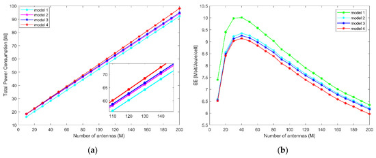
Figure 4.
(a) Total power for K = 10 and varying M and (b) EE versus M for the different power model.
Figure 5 shows the corresponding EE with different power allocation schemes. The simulation result manifests that the proposed algorithm outperforms all reference schemes and provides the highest EE, followed by maxprod, and then equal power allocation irrespective of the value of M. The bottom curve is obtained from max-min power allocation, which is almost flat after the peak as fairness in SE compensates for the vast loss of EE. Quantitatively speaking, the performance gap is substantial for M = 40 around 3.75 Mbits/Joule/cell between the proposed and maxprod scheme. The use of the proposed algorithm increases EE performance by 10–30% over the reference schemes in the interval M = [10,100]. Then, the performance gap between curves continues to narrow after peaks. The essence of this result is that the negative impact incurred by equipping excessive antennas dominates over the gain from power allocation intended for EE optimization due to the fact that a modest logarithmic SE gain already could not compensate for the corresponding antenna energy consumption. It is worth mentioning during the simulation that the maxprod algorithm is of a high cost of computation, which underperforms the proposal in spite, indicating fully the superiority of the Dinkelbach-like algorithm.
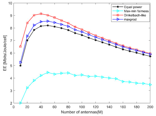
Figure 5.
EE versus M with different power allocation schemes.
The curves in Figure 6 represent the average sum SEs. Compared to the EE case, when M increases, the array gain causes SE to grow monotonically without boundary. The top curve is still obtained from the proposed algorithm, which means performing well in both EE and average sum SE. In the meanwhile, the gain gap between the maxprod and the proposal narrows gradually. Fortunately, the proposal still outperforms slightly up to 1–20%. The interpretation is that the favorable propagation achieved by having many BS antennas makes the noncoherent interference between each pair of UEs sufficiently small, while the Dinkelbach-like algorithm detrimentally enjoys such a benefit as a result of initialization of interference. In other words, some saturation effect appears and the marginal gain in average sum SE of the Dinkelbach-like algorithm gradually diminishes when M goes to infinity. In fact, the energy-efficient massive MIMO will not equip such infinite antennas regardless of the consideration of physical constraints or the conclusion followed from above.
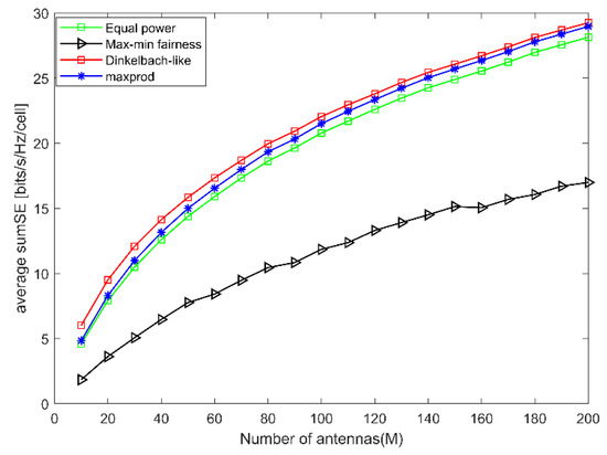
Figure 6.
Average SE versus M with different power allocation schemes.
The general observation from Figure 7 is that the cumulative distribution function (CDF) curve with the proposal is mostly to the maxprod power allocation curve, which, in turn, is to the right of the equal scheme, and then the max-min fairness. In what follows, most UEs will, statistically speaking, achieve better performance with the proposal than with the other schemes. In addition, Figure 7 demonstrates implicitly the performance matrix loss of fairness as compared to the max-min scheme as the fairness baseline. It should be observed that 9% and 18% of UEs perform less well than the corresponding schemes at the tails of the CDF curves. However, we only sacrifice a few percentages of UEs with poor channels in turn to the gain in EE and sum SE, even if there are as many as 18% UEs. It is cost-efficient as far as EE optimization is considered, and most UEs are better off statistically.
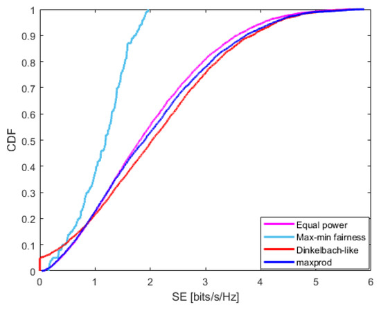
Figure 7.
CDF of the SE per UE versus M with different power allocation schemes.
Figure 8 is obtained with two value sets of simulation parameters in Table 1. As we see, the other is set by scaling the hardware’s power consumption by a factor of 2 wherein computational efficiencies are improved and more energy-efficient transceiver chains are used, which are expected to improve in the future. Intuitively, the general trends for both value sets are the same. Still, the improved hardware system overwhelms the power allocation schemes absolutely, identifying directly a way to improve EE essentially. It indicates that we can either offload data traffic or improve the computation hardware to accelerate the speed of computation at the BS side, as well as exploit more energy-efficient transmit chains. In addition, the power allocation scheme we proposed prevails over the rest irrespective of system parameters. In other words, the proposed algorithm can be extended to be used in future, more efficient systems and performs well off.
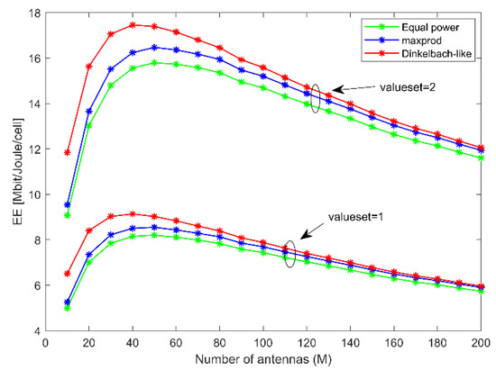
Figure 8.
EE versus M with two sets of hardware systems.
5.3. Computation Complexity Analysis
The solution process is to solve a sequence of auxiliary problems, indexed by the parameter . Hence, the overall computational complexity counts on the complexity of each individual subproblem and the outer loop convergence about updating parameter , which is confirmed to exhibit at least a two-order convergence rate. Therefore, the subproblem’s computational complexity dominates the overall computational complexity. Usually, the floating-point operation (flop) indicates the computational complexity. A real addition, multiplication, or division is counted as one flop [24]. In the algorithm, the pretreatment requires about 2LK+2 flops. In addition, one execution of steps in Algorithm 2 takes approximately flops assuming and are the iteration times of two while-loops. Consequently, the overall complexity approximates , namely low polynomial complexity thanks to the super-linear convergence rate, where and is the iteration times for the parameter. In contrast, if the objective is nonconcave, then the complexity required for global optimal resource allocation is, in general, exponential. Moreover, the max-min fairness solves linear feasibility subproblems in the bisection search, which requires , while the maxprod solves geometric programs based on the interior point method, which requires polynomial executions and each execution entraining flops. Obviously, the proposed algorithm pays off in terms of EE and is more computationally efficient than the maxprod.
6. Conclusions
For the multi-cell multi-user massive MIMO downlink energy efficiency optimization in an interference-limited scenario, we propose a sub-optimal Dinkelbach-like algorithm with limited complexity under the constraint of maximum transmit power. To make the scheme more practical, we adopt the more realistic power consumption model and fully consider the impact of dynamic power terms. The simulation results confirm the rationality of the proposed algorithm, which can jointly increase EE and the average sum of SE with lower complexity, and meanwhile obtain satisfactory performance in SE fairness. Hence, it is a candidate as a computationally efficient method adapted for the low-latency requirement of the sixth-generation communication, as the proposed algorithm strikes a good balance between performance and complexity.
As we can see, SE grows with antenna number without bound. However, equipping excessive antennas not only brings extra power consumption but also increases the complexity of system design. Hence, in future work, it is optional to consider the joint optimization of antenna selection and power allocation to promote energy conservation at the marginal loss of SE. In addition, if we want to reach a higher SE and EE in massive MIMO, the simulation result shows that it is wise to search for more energy-efficient transmit chains. Noticeably, power allocation is irreplaceable as a method that improves EE and SE through the rational allocation of resources within a limited resource budget. Therefore, power allocation is of significant consideration in energy-efficient optimization whatever the optimized system design is in future work.
Author Contributions
Conceptualization, H.L. and H.D.; data curation, H.L. and G.L.; formal analysis, H.L., Y.Y. and J.Z.; project administration, H.L.; resources, H.D.; software, H.L., Y.Y., Z.Z. and J.Z.; supervision, H.D. and G.L.; writing—original draft, H.L. and Z.Z.; writing—review and editing, H.L. All authors have read and agreed to the published version of the manuscript.
Funding
This research received no external funding.
Institutional Review Board Statement
Not applicable.
Informed Consent Statement
Not applicable.
Data Availability Statement
Not applicable.
Conflicts of Interest
The authors declare no conflict of interest.
References
- Zong, B.; Fan, C.; Wang, X.; Duan, X.; Wang, B.; Wang, J. 6G Technologies: Key Drivers, Core Requirements, System Architectures, and Enabling Technologies. IEEE Veh. Technol. Mag. 2019, 14, 18–27. [Google Scholar] [CrossRef]
- Buzzi, S.; Chih-lin, I.; Klein, T.E.; Poor, H.V.; Yang, C.; Zappone, A. A Survey of Energy-Efficient Techniques for 5G Networks and Challenges Ahead. IEEE J. Sel. Areas Commun. 2016, 34, 697–709. [Google Scholar] [CrossRef] [Green Version]
- Marzetta, T.L. Noncooperative cellular wireless with unlimited numbers of base station antennas. IEEE Trans. Wirel. Commun. 2010, 9, 3590–3600. [Google Scholar] [CrossRef]
- Zappone, A.; Sanguinetti, L.; Bacci, G.; Jorswieck, E.; Debbah, M. Energy-Efficient Power Control: A Look at 5G Wireless Technologies. IEEE Trans. Signal Process. 2016, 64, 1668–1683. [Google Scholar] [CrossRef] [Green Version]
- Khodamoradi, V.; Sali, A.; Messadi, O.; Salah, A.A.; Al-Wani, M.M.; Ali, B.M.; Abdullah, R.S.A.R. Optimal Energy Efficiency Based Power Adaptation for Downlink Multi-Cell Massive MIMO Systems. IEEE Access 2020, 8, 203237–203251. [Google Scholar] [CrossRef]
- Kwon, J.H.; Cho, J.; Yu, B.; Lee, S.; Jung, I.; Hwang, C.; Ko, Y.C. Spectral and energy efficient power allocation for MIMO broadcast channels with individual delay and QoS constraints. J. Commun. Netw. 2020, 22, 390–398. [Google Scholar] [CrossRef]
- Salh, A.; Shah, N.S.M.; Audah, L.; Abdullah, Q.; Jabbar, W.A.; Mohamad, M. Energy-Efficient Power Allocation and Joint User Association in Multiuser-Downlink Massive MIMO System. IEEE Access 2020, 8, 1314–1326. [Google Scholar] [CrossRef]
- Li, H.; Wang, Z.; Wang, H. Power Allocation for an Energy-Efficient Massive MIMO System With Imperfect CSI. IEEE Trans. Green Commun. Netw. 2020, 4, 46–56. [Google Scholar] [CrossRef]
- Zhang, J.; Deng, H.; Li, Y.; Zhu, Z.; Liu, G.; Liu, H. Energy Efficiency Optimization of Massive MIMO System with Uplink Multi-Cell Based on Imperfect CSI with Power Control. Symmetry 2022, 14, 780. [Google Scholar] [CrossRef]
- You, L.; Xiong, J.; Zappone, A.; Wang, W.; Gao, X. Spectral efficiency and energy efficiency tradeoff in massive MIMO downlink transmission with statistical CSIT. IEEE Trans. Signal Process. 2020, 68, 2645–2659. [Google Scholar] [CrossRef] [Green Version]
- Ngo, H.Q.; Larsson, E.G.; Marzetta, T.L. Aspects of favorable propagation in Massive MIMO. In Proceedings of the 2014 22nd European Signal Processing Conference (EUSIPCO), Lisbon, Portugal, 1–5 September 2014; pp. 76–80. [Google Scholar]
- Jin, S.N.; Yue, D.W.; Nguyen, H.H. On the Energy Efficiency of Multi-Cell Massive MIMO With Beamforming Training. IEEE Access 2020, 8, 80739–80754. [Google Scholar] [CrossRef]
- Bonsu, K.A.; Zhou, W.; Pan, S.; Yan, Y. Optimal power allocation with limited feedback of channel state information in multi-user MIMO systems. China Commun. 2020, 17, 163–175. [Google Scholar] [CrossRef]
- Gao, H.; Su, Y.; Zhang, S.; Diao, M. Antenna selection and power allocation design for 5G massive MIMO uplink networks. China Commun. 2019, 16, 1–15. [Google Scholar] [CrossRef]
- Honggui, D.; Jinli, Y.; Gang, L. Enhanced Energy Efficient Power Allocation Algorithm for Massive MIMO Systems. In Proceedings of the 2019 IEEE 11th International Conference on Communication Software and Networks (ICCSN), Chongqing, China, 12–15 June 2019; pp. 280–285. [Google Scholar]
- Paulraj, A.J.; Papadias, C.B. Space-time processing for wireless communications. In Proceedings of the 1997 IEEE International Conference on Acoustics, Speech, and Signal Processing, Munich, Germany, 21–24 April 1997; pp. 49–83. [Google Scholar]
- Emil, B.; Jakob, H.; Luca, S. Massive MIMO Networks: Spectral, Energy, and Hardware Efficiency; Now Publishers Inc.: Delft, The Netherlands, 2017. [Google Scholar]
- Hochwald, B.M.; Marzetta, T.L.; Tarokh, V. Multiple-antenna channel hardening and its implications for rate feedback and scheduling. IEEE Trans. Inf. Theory 2004, 50, 1893–1909. [Google Scholar] [CrossRef]
- Marzetta, T.L. Fundamentals of Massive MIMO; Cambridge University Press: Cambridge, UK, 2016. [Google Scholar]
- Liu, Z.; Li, J.; Sun, D. Circuit Power Consumption-Unaware Energy Efficiency Optimization for Massive MIMO Systems. IEEE Wirel. Commun. Lett. 2017, 6, 370–373. [Google Scholar] [CrossRef]
- Zappone, A.; Jorswieck, E. Energy Efficiency in Wireless Networks via Fractional Programming Theory; Now Publishers Inc.: Delft, The Netherlands, 2015. [Google Scholar]
- Dinkelbach, W. On nonlinear fractional programming. Manag. Sci. 1967, 13, 492–498. [Google Scholar] [CrossRef]
- Ngo, H.Q.; Tran, L.-N.; Duong, T.Q.; Matthaiou, M.; Larsson, E.G. Energy efficiency optimization for cell-free massive MIMO. In Proceedings of the 2017 IEEE 18th International Workshop on Signal Processing Advances in Wireless Communications (SPAWC), Sapporo, Japan, 3–6 July 2017; pp. 1–5. [Google Scholar]
- He, S.; Huang, Y.; Yang, L.; Ottersten, B. Coordinated multicell multiuser precoding for maximizing weighted sum energy efficiency. IEEE Trans. Signal Process. 2013, 62, 741–751. [Google Scholar] [CrossRef]
Publisher’s Note: MDPI stays neutral with regard to jurisdictional claims in published maps and institutional affiliations. |
© 2022 by the authors. Licensee MDPI, Basel, Switzerland. This article is an open access article distributed under the terms and conditions of the Creative Commons Attribution (CC BY) license (https://creativecommons.org/licenses/by/4.0/).