Scalable Post-Processing of Large-Scale Numerical Simulations of Turbulent Fluid Flows

Abstract

Military, space, and high-speed civilian applications will continue contributing to the renewed interest in compressible, high-speed turbulent boundary layers. To further complicate matters, these flows present complex computational challenges ranging from the pre-processing to the execution and subsequent post-processing of large-scale numerical simulations. Exploring more complex geometries at higher Reynolds numbers will demand scalable post-processing. Modern times have brought application developers and scientists the advent of increasingly more diversified and heterogeneous computing hardware, which significantly complicates the development of performance-portable applications. To address these challenges, we propose Aquila, a distributed, out-of-core, performance-portable post-processing library for large-scale simulations. It is designed to alleviate the burden of domain experts writing applications targeted at heterogeneous, high-performance computers with strong scaling performance. We provide two implementations, in C++ and Python; and demonstrate their strong scaling performance and ability to reach 60% of peak memory bandwidth and 98% of the peak filesystem bandwidth while operating out of core. We also present our approach to optimizing two-point correlations by exploiting symmetry in the Fourier space. A key distinction in the proposed design is the inclusion of an out-of-core data pre-fetcher to give the illusion of in-memory availability of files yielding up to 46% improvement in program runtime. Furthermore, we demonstrate a parallel efficiency greater than 70% for highly threaded workloads.

1. Introduction

Computational fluid dynamics (CFD) has become an important tool for understanding ubiquitous phenomena, such as compressible high-speed turbulent boundary layers, which are critical for efficient high-speed flight. However, the fundamental understanding of such flows, from preparing and running these simulations to ultimately gathering valuable insights from the vast amounts of data generated, presents unique computational challenges. For example, a modest 4D simulation (3D space + time) can generate 12 billion data points with simple geometry. On the other hand, we capture smaller-scale motion at higher Reynolds numbers. We account for strong surface curvature effects in complex geometries that can generate 2 trillion data points (16 terabytes of raw data). Soon, we aim to simulate flow at even more complex geometries by increasing Reynolds numbers (i.e., large-scale systems) which will continue to exponentially raise the need for efficient post-processing utilities to extract valuable scientific insights from these simulations.

Complicating factors for the post-processing of these large-scale, numerical simulations are the continuously growing number of diversified computing infrastructure [1,2] and heterogeneous processors [3]. This adds more challenges to the development of portable scientific applications [4]. Recent and upcoming supercomputers have nodes with multiple CPU sockets with many cores across each (not to be confused with the literal “many-core” micro-architecture advocated by Intel in the past), and potentially accelerators, such as FPGAs, GPUs, and other custom ASICS connected to each socket over standard PCIe, or another proprietary interconnect. The wide variety of computational accelerators and connection technologies introduces complex NUMA effects and compounds the available programming models [5]. Achieving peak performance and strong scaling requires careful attention to micro-architectural differences between computing devices which inevitably introduce additional complexities. With the growing sizes of numerical simulations, copying the whole dataset into the main processor memory pool could be impractical or impossible in most cases where terabytes of data are managed. To tackle this problem, one could consider out-of-core computing [6,7,8,9]; computing on data stored in slower media such as hard drives and moving these to and from main memory as needed by the application. Some approaches have been proposed in the past, such as DIY2 by Morozov and Peterka [10] which could operate on in-core and out-of-core datasets similarly by abstracting away the movement of data via an MPI layer. The interfaces outlined by the authors are flexible and relatively simple to use, but DIY2 experiences a degradation in strong scaling performance when operating from in-flash data. This leads to a drop in parallel efficiency to 64% (comparing performance at 128 processes to a baseline of 32 processes). This loss of strong scaling performance contrasts with its execution for in-memory data, which achieves 91% parallel efficiency. Further complicating matters, the application runtime grows by 1.59–2.27× when operating from non-volatile memory drives. Given the continuously growing size of datasets generated by the CFD community, this situation poses challenges. In addition, with increasing scientific requirements, the time available for analysis is often kept constant. Brezany et al. [6] promoted the highly optimized file read/write to enable out-of-core computing and contrasted other approaches, including virtual memory, which is often unavailable in supercomputers. Tuned file IO could potentially reduce runtime by 4–20× [11] compared to relegating data loads and memory swaps to the OS (the virtual memory approach). The proposed runtime also reinforced this latter fact, and language support by Brezany et al. [7], which was crucial to the MPI IO predecessor PASSION [12].

Based on these growing nuances, application developers should use portable abstractions when writing scientific software to allow programmer productivity and good performance regardless of available hardware resources on the current rise of the heterogeneous compute node. Many such abstractions have been developed, with varying levels of performance, ease of use, and vendor acceptance. Some of these abstractions include SYCL [13], RAJA [14], OpenMP [15], OpenACC [16], Legion [17], Kokkos [18], and many others omitted. Both OpenACC and OpenMP follow a compiler-pragma-based approach, whereas Legion, RAJA, SYCL, and Kokkos are built on top of C++ abstractions [19]. The OpenMP standard is widely implemented and supported among compiler vendors for its generic and unobtrusive interface that allows incremental porting of applications. This being said, directive-based approaches live outside the type system, limiting compiler optimizations and visibility across layers of abstractions. On the contrary, OpenACC has not experienced such widespread adoption and is confined chiefly to PGI compilers and Nvidia devices. With regards to the C++ abstractions, SYCL has gathered significant interest recently. Mainly due to Intel announcing it would base its oneAPI [20] initiative on a superset of SYCL with plans to standardize the extensions. In addition, AMD has invested significantly in the SYCL initiative through its hipSYCL implementation. Codeplay [21] recently announced support for Nvidia devices via an experimental PTX generator in addition to its support for AMD and other CPU targets. That being said, SYCL is a verbose approach that ends up tying any application to the availability of an SYCL implementation that depends on vendor support. Rather than requiring vendor-specific support, Kokkos [18] (and similarly RAJA [14]) take advantage of the rich abstractions achievable in C++ via templates and other composable abstraction mechanisms. This enables a platform-agnostic platform that only requires recompiling for a given platform. What is more, Kokkos provides an abstraction over memory accesses and layouts [18], crucial to ensuring performance portability across CPUs and GPUs.

To address the requirements of post-processing large-scale computational fluid dynamics simulations in a heterogeneous high-performance computing system, we have proposed a scalable, performant, portable, and distributed library capable of handling the post-processing of large-scale simulations [22]. This is achieved while relieving the domain expert from the burden of low-level computational details of vital importance to achieving high-performance and strong scaling [22]. This is achieved through a modern and opinionated abstraction system that hides unnecessary complexity from the scientific application developer. The current approach builds over two significant abstractions: modular operations and a distributed flow field. Previous work has shown that these abstractions can be platform-independent [22]. In this work, we demonstrate that these can be language-independent by implementing these in Python in addition to the existing C++ implementation targeting different parallel programming models. While current efforts are targeting the implementation of GPU capabilities in Aquila (which would be published elsewhere), the present manuscript is focused on CPU performance studies. We demonstrate that scalability can be achieved independent of implementation details as long as certain specific concepts are always present in the implementation. For instance, asynchronous pre-fetch and concurrent operation scheduling are crucial for strong scaling, parallel efficiency, and quick turnover. The C++ implementation leverages Kokkos and MPI, whereas the Python implementation may target multiple NumPy compatible libraries. The C++ distributed flow field can leverage any distributed computing library wrapped around the Aquila Communicator interface, and it targets Kokkos as its performance portability layer. Kokkos enables transparent execution and performance portability on GPUs, CPUs, and other compute devices from multiple hardware vendors while abstracting away the distributed memory layer. It also permits the adoption of nearly any distributed-memory communication library. That said, MPI [23] is the only currently supported backend as of the time of writing. The proposed library approach is portable and can scale down from large supercomputers to small clusters to workstations to laptops with no changes to the source code. It also supports running in a pure, shared memory context without MPI. The Python implementation leverages the widely adopted NumPy array interface to enable a generic interface that can accept CuPy, NumPy, Dask, and other compatible interfaces. Distributed communication is handled via MPI. Thus, we present a generic interface for both the C++ and Python implementations, leveraging the strengths and addressing the weaknesses of both languages. In the present work, we outline a general language-independent group of principles and ideas and implement these in two vastly different languages, C++ and Python, to highlight the language independence of these guidelines. A noteworthy difference in our design is the scalable inclusion of asynchronous, out-of-core post-processing pipelines with data pre-fetch to give the illusion of in-memory availability of said data. We highlight the strong scaling performance of our proposed solution while operating on out-of-core datasets, enabled primarily through optimized, scalable, and asynchronous file-based IO. Additionally, we show scaling results on porting a post-processing analysis from a usability and performance point of view. We also expect an essential impact of the present contribution beyond the CFD community, since the bottom line of the proposed approach is “dealing efficiently and speedily with a huge amount of numerical data”, and big data problems can be found everywhere.

2. Design Rationale and Implementation Details

2.1. Design Rationale

We propose four main, language-independent design principles:

• Provide as much information as possible at “compiling time”. In interpreted languages, this can be achieved via dynamic planning that adjusts underlying libraries analogous to the FFTW planning and runtime adaptive scheme [24,25,26,27,28,29,30].
• The underlying mesh is mostly structured. Certain operations on partially structured meshes or hybrids can be supported if the node connectivity is known. For instance, many Eulerian, time-averaged quantities can be trivially extended to unstructured meshes even without connectivity information. If turbulence statistics involves flow gradients, numerical integration, fluxes, etc., the connectivity information must be included.
• A minimal amount of temporal data was kept in the main memory. This enables scaling to larger datasets (larger simulation time).
• File formats are bound to change and have evolved significantly throughout the years.

Each of these principles has steered our development from core areas to user-facing interfaces. As with many high-performance libraries, we focus on maximizing parallel slack to enable concurrent and independent execution paths with minimal synchronization points. This philosophy enables strong scaling and inspires the asynchronous operation inclusion model in the Python implementation. It also serves as the basis for the guideline that operations that may run in parallel should be allowed. This drives the independent processing of flow fields as all operations can be done embarrassingly parallel to the final reduction operations. In the C++ version, we followed a more traditional approach by incorporating domain decomposition in a distributed memory programming model and enabling parallel operations to execute concurrently in a threaded pipeline. We approach domain decomposition through a shared memory approach to maximize resource sharing and utilization in the Python implementation. As we will see, sharing a thread pool for pre-fetch, processing, and coordination operations enables efficient resource utilization in an out-of-core context.

We will discuss three implementations in the present work, a C++ implementation, and two Python implementations. The C++ implementation leverages Kokkos to abstract data memory layouts and offers the potential of GPU targeting without major code changes. The data pre-fetcher is implemented using the pipeline provided by Threading Building Blocks (TBB) [31]. We also integrate processing stages as pipeline stages to enable concurrency and out-of-order, asynchronous execution. In Python, we implement a hybrid parallel decomposition strategy allowing independent processing of flow fields by workers (implemented using MPI [32,33,34]) and leverage parallelism in operations via concurrent futures patched with TBB [35], NumPy [36], and Numba [37]. This enables operations that would not scale as well across distributed memory, such as Fast Fourier Transform (FFT) and complex stencil operations. These operations are more efficient in a shared memory context. Further, as new operations are introduced, they are submitted as asynchronous operations (futures) into one of several pools initialized by the TBB pool. Worker threads then execute these operations, and a thread may steal work from other threads as needed. Each operation may also be parallelized internally and leverage the same pool as the tasks. This approach scales the available parallel slack as more operations are implemented, which leads to better resource utilization. The operations are submitted to a TBB thread pool, so the available hardware resources are not oversubscribed, and irregular work is automatically load-balanced without a central dealer.

Our library also provides a set of algorithms and standard post-processing utilities that offload work to the underlying Kokkos and Distributed Volume internals, providing proper CFD post-processing operations, including time-averaged flow calculation, Root Mean Square (RMS), cross-correlations, two-point correlations, and power spectra of fluctuations. Standard, stencil-like communication patterns are also supported, enabling the straightforward implementation of volumetric gradients, opening the door for additional functionalities. The algorithms leverage the Kokkos API and can be executed on CPUs and GPUs by simply recompiling the application with a different Kokkos backend.

As a final note, compiling code on supercomputers is often “free”, as some of the guidelines behind the design principles suggest. Free doe not mean a lack of data centers or the cost of energy consumption, but a computing unit that researchers can use. In addition, compiling a small post-processing run is often dwarfed in time by the actual runtime of the code. However, the compiler produces the best binaries when given most of the critical information. These include array dimensions, loop boundaries, array alignment and padding, memory access patterns, and interactions between components. Therefore, this method needs to be compiled with a post-processing application, including processing the dimensions of the volume. Of course, this leads to potential annoyance. However, getting good performance on complex architectures is worth a few extra seconds on the command line. This process also configures Kokkos to run on a specific backend. When link-time optimization is enabled, the compiler can optimize object files to provide the best performance at the cost of increased compilation time. As part of this data-driven combination, the user also defines the distribution layout of the volume, which can be divided along with the flow direction of the fluid flow and the wall-normal. This allows index constants to be precomputed, reducing runtime pressure from the CPU backend.

Another key difference is its forward-looking approach to storage needs. The size of the dataset keeps increasing, and the storage within the node is more or less constant. So, assume that only 1 or 2 timesteps are in memory or read at any given time. This can cause problems when scaling on supercomputers due to the high latency of parallel file systems. Our plan of attack draws inspiration from the latency hiding philosophy in GPUs to address this. Traditional Graphics Processing Units often exhibit very high latencies in data fetching and overcome this by oversubscribing the hardware and allowing multiple execution contexts to be in flight simultaneously. This contrasts with CPUs which incorporate complex machinery to avoid pipeline stalls and reduce latency as much as possible for a single thread of execution. To achieve latency hiding, we include a parallel pipeline from the Threading Building Blocks (TBB) multithreading library. It is analogous to the approach followed by GPUs and CPUs, although neither serves as a perfect analogy. The pipeline maintains a compile-time-defined number of concurrent flow fields at any pipeline stage, thus allowing resources to be invested where they are needed the most and tolerating latencies induced at network-bound stages. Therefore, it is designed to execute significant amounts of work per file read to hide the latency of reading these over a network link. This is analogous to the way GPUs hide outstanding loads and other high-latency operations by hiding these with work [38].

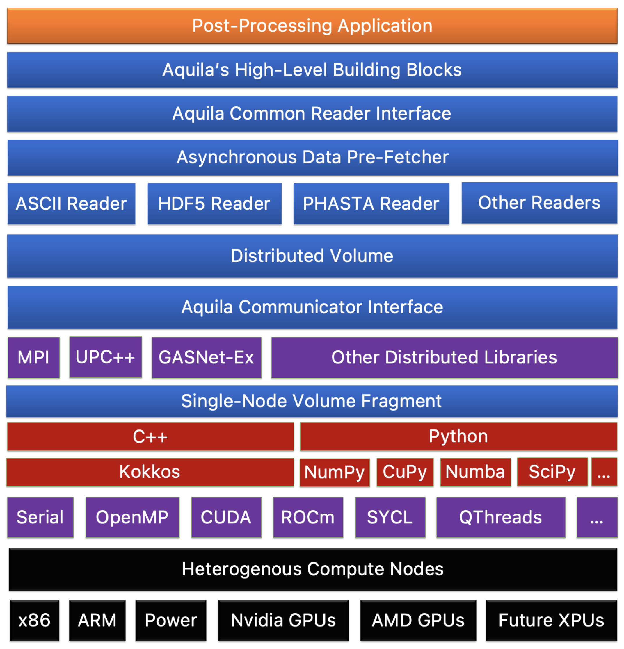
The fourth design principle is related to many file formats and their constant evolution. As with hardware heterogeneity (or, some would affirm, even more critical), the amount of file formats available to application developers is far too large even to keep up. Furthermore, many software packages, libraries, and scientific domains have vastly differing IO backends, making choosing an IO format as necessary as the language in which an application is programmed. The proposed methodology provides a modular interface for IO for distributed memory communication to address this fact. Depending on the need, any given file format can be supported if it implements a Writer or Reader, which is a customization point between Aquila and any other file format. For instance, data stored in a NetCDF file can be read by an application writing to HDF5 or vice versa. This format-resiliency to IO requirements enables flexible interfaces sharing a common, high-performance computational core. These components are presented in a simplified schematic in Figure 1 (taken from [22]; reprinted by permission of the American Institute of Aeronautics and Astronautics, Inc.).

2.2. Implementation Details

The Python implementation supports Python 3.8 and above. Due to the design, it was upgraded to support higher standards and more recent Python versions. The C++ implementation requires C++14 (it was initially developed to support C++17, but was later downgraded due to lack of support in some supercomputers) with extensive use of compile-time operations. Kokkos is extensively used to implement volume stripes and algorithms by allocating arrays through Kokkos and expressing functions using the Kokkos programming model. By ensuring separation of concerns, backend enhancements propagate gains to higher levels of abstractions. For instance, improvements to the low-level operations result in progress across all algorithms that leverage these. For example, modifications to elementwise operations propagate to all algorithms that require elementwise operations without any changes to the source code.

We promote vectorization at these by providing the compiler with power-of-two loop bounds and compile-time-known memory layout. To facilitate disjoint memory spaces in accelerators with discrete memory pools or program addressable multi-tiered memory, we implement a memory state flagging scheme that tags memory as dirty when a mirror allocation is accessed from a different device. Before accessing memory, this flag is checked, cleaning the memory if necessary by transparently copying the memory across devices. The mirror allocation matches the host memory layout (including padding), enabling transferring memory without intermediate buffers. Care is taken to minimize expensive transfers, and these are often limited to data assignment operations at file read/write. These transfers are denoted as indispensable transfers since the implementation of Reader/Writer currently involves an intermediate buffer. (This is not strictly necessary, given column-major layouts are used for GPUs, we favored a row-major read/write buffer. The overhead is minimal as these operations can be performed asynchronously.)

The most communication-intensive operation is the two-point correlation (TPC), which requires “pencil” communication (a pencil is defined for this job as a single “row” of data). It can be inferred from the last statement that it introduces additional parallelism by allowing multiple groups of ranks to work independently on a single timestep of the simulation, avoiding synchronizing many processes. We use parallelism at the distributed, thread, and instruction levels. Any scientific application that expects proper scaling and good performance must use parallelism at the appropriate level by allowing the user to specify the number of stripes. At runtime, the user provides multiple stripes as the number of ranks, which this code uses internally to provide independent sets of ranks for independent progress. When time reduction is required, the groups must be synchronized at the end of the pipeline. Suppose a pipeline contains multiple post-processing algorithm requests. Each “reduce” is issued as an asynchronous “reduce”, allowing better overlap of computation and communication if the underlying distributed runtime supports it. This is a common theme across many aspects of this code implementation, and we try to provide as many opportunities for optimization and concurrency as possible. This allows Aquila to take advantage of many options that domain experts should not know but must exploit to achieve good scalability and optimal performance for a given hardware/software stack.

2.3. File Formats and Supported Operations

This section describes our support for different file formats and how additional formats can be supported with relative ease. Furthermore, we will also discuss some of the supported families of operations and limitations imposed by design decisions in the C++ and Python implementations. We define an opinionated internal format for all arrays and “readers” that convert from native file format data layouts to this internal format. We support writing to VTK and HDF5 as current output formats, with the HDF5 writing backend expressing arrays following the interior layout for efficiency. Consequently, a reader can have any arbitrary implementation if it generates an array that adheres to the internal file format. We currently support reading from VTK (implemented to support OpenFOAM), HDF5, and ASCII file formats. Although a reader can execute arbitrary code, the results are optimal when the reader is kept to a bare minimum and avoids any locking due to the asynchronous nature of the pre-fetcher. This becomes particularly important in the Python implementation, where leveraging function calls that release the Global Interpreter Lock [39] is highly beneficial.

Currently, the C++ and Python implementations have diverged in terms of the supported operations, but it could be said that the Python implementation supports a super-set of the C++ operations. The C++ implementation (denoted as Aquila V1, although the two versions have minor changes) supported basic post-processing routines, including cross-correlations, mean flow calculations, fluctuations, RMS, and two-point correlations. We present two Python implementations (Aquila V2 and Aquila V2.1) with two notable changes between V2 and V2.1. First, the two-point correlation operation was updated from V1 to V2.1. V1 implemented a custom dot product-based TPC, leveraging a custom small vector dot product written using AVX2 intrinsics. We updated this implementation to leverage MKL-batched matrix-matrix operations. This increased the arithmetic intensity, better utilized the available memory bandwidth, and increased the available parallelism. For V2.1, the two-point correlation was re-written to leverage FFTs from FFTW [24,25,26,27,28,29,30] if available with an Eigen fallback [40], and we also implemented an asynchronous operation submission engine (we denote this engine as the Aquila Futures Interface [AFI]). The AFI is implemented using Python futures and a TBB pool. The AFI combines these two results in a decentralized execution pool capable of handling the unbalanced parallelism and the combination of nested task and data parallelism from the asynchronous task pool. Furthermore, this architecture simplifies the inclusion of user-defined calculations that may leverage Aquila’s core computational engine and abstractions as first-class citizens. It is also worth noting that although we present a set of available functionalities, the library includes (either directly or allows for straightforward implementation) a large number of flow parameters including those dependent on gradients, integrals, and other higher-order statistics.

Optimizing 3D Two-Point Correlations, the Heart of Aquila’s Coherent Structure Detection Approach

The naive implementation for a two-point correlation requires $\mathcal{O}(N_t\ast N_x\ast N_y\ast N_z^2)$ floating point operations with $N_z$ calls to a rotate algorithm (shifting elements in the volume along z). One notable improvement can be achieved if at least one coordinate exhibits homogeneity (for instance, wall-bounded flows are often modeled with periodical boundary conditions on at least one dimension, although the algorithm is generally applicable to any volumetric physical quantity with at least one homogeneous dimension) by leveraging the convolution theorem [41,42] which translates the problem from the physical to the Fourier domain. Focusing on the gains along the homogeneous dimension and given the input is a real input, we can exploit the natural symmetry in the Fourier domain (complex conjugate symmetry) and preserve the data size even when considering complex values since only $1/2$ of the frequencies are considered. Further, the FFT’s complexity is proportional to $\mathcal{O}\left({log}_{2}N\right)$. Given only half the frequencies are considered, this yields a complexity of $\mathcal{O}\left({log}_2{N}_z/2\right)$ and a storage requirement of $N_z$ (complex numbers occupy twice the memory footprint of a real scalar). This also reduced the number of complex operations involved since only $N_z/2$ complex multiplications are required. Consequently, the spanwise complexity is reduced from $\mathcal{O}\left(N_z^2\right)$ to $\mathcal{O}\left(\frac{N_z}{2}{log}_2\left(\frac{N_z}{2}\right)\right)$. By preserving the data size and reducing data movement, we have thus increased the arithmetic intensity making the TPC calculation much more efficient in modern computing hardware such as CPUs with wide vectors and GPUs. The overall complexity can be assumed to be $\mathcal{O}\left(N_t\ast N_x\ast N_y\ast \frac{N_z}{2}{log}_2\left(\frac{N_z}{2}\right)\right)$ (although the $1/2$ factors should not appear in big-$\mathcal{O}$ notation, we included these to highlight important savings attained by exploiting symmetry in the Fourier domain).

This scaling behavior is much more favorable and, even after accounting for increased FLOP count in complex arithmetic, could lead to a 20× increase in performance for the largest case considered in the present work. If we did not exploit the symmetry present in the Fourier domain, we would double the intermediate data size and would cap the theoretical speedup to 9× even assuming infinite bandwidth. This highlights the power of algorithm selection, incorporating domain-specific knowledge and proper numerical implementation so as to reduce the computational cost.

The general algorithm for the real-to-complex, FFT-based, two-point correlation can be derived by noting that for any real input, $f\left(x\right)$, the Fourier transform, $\mathcal{F}\left(\chi \right)$, is symmetric (i.e., $\mathcal{F}\left(\chi \right)=\mathcal{F}(-\chi )$). Thus, we can get away with using a real input, avoiding an intermediate buffer to cast the data to a complex data type, and outputting only half of the Fourier transform. The two-point correlation, R, is then expressed as,

$$R\left(x\right)={\mathcal{F}}^{-1}\left[\mathcal{F}\left(\chi \right){\mathcal{F}}^{\ast }\left(\chi \right)\right]$$

where ${\mathcal{F}}^{\ast }\left(\chi \right)$ is the complex conjugate of the Fourier transform and ${\mathcal{F}}^{-1}$ is the inverse Fourier transform. Note, that when taking the Fourier transform we only preserve the positive and zeroth terms since the negative frequencies are assumed to be symmetric with respect to the origin. This enables the complex buffer to be of equal size to the real buffer while reducing the amount of data moved and ensuring a higher arithmetic intensity while operating in the frequency domain. In summary, we have transformed a spatial correlation with an element-wise frequency multiplication. If the problem lacks a homogeneous dimension, a straightforward fallback can be implemented which computes the TPC in the physical domain. The main advantage of the Fourier space against a well-implemented TPC calculation in the physical domain is performance as we have alluded throughout the discussion. If a validated, high-performance FFT library is available for a given system (which often is), the implementation is also much more straightforward and less prone to mistakes since it contains fewer operations and data movements.

3. Performance Analysis

3.1. Computational Environment

Characterizing the portability and the performance portability of any piece of software requires studying it under different loads, environments, and stressing different areas in realistic manners. To this end, we chose 4 platforms ranging from an aging platform to a state-of-the-art platform. The systems chosen have very different characteristics in their compute elements, filesystems, and interconnects. Coupled to different benchmarks, these four systems provide a realistic view on attainable performance for our proposed post-processing approach. It is worth noting that although some of these platforms have GPU resources, we have limited our study to general purpose CPUs to reduce the number of variables and tuning parameters present.

3.1.1. Cray XE6m—Copper

We show the results of a run performed on the Copper Cray XE6m system. The nodes in the XE6m featured dual-socket AMD Interlagos Opteron, each with 16 floating-point modules and 32 integer cores. This micro-architecture oversubscribed floating point units on a 2 to 1 ratio. Although this architecture is old, it provides a suitable test environment for oversubscribed architectures. Still, challenges include oversubscribing computing resources and limited access to storage servers, as Copper has only 1 Lustre Metadata Target Servers (MDTs) and 20 Object Storage Targets (OSTs). Each compute node has 60 GB of accessible RAM with a nominal clock speed of 2.3 GHz per core. Nodes are interconnected via Cray Gemini interconnects, providing a 3D torus topology. The results presented were run on compute nodes running Cray Linux with Cluster Compatibility Mode (CCM) enabled. We test Aquila from a single node, up to 128 nodes (maximum number of nodes per job in Copper, i.e., seven node doublings).

GCC 4.9 was the only available compiler that supported all required C++. Therefore, we chose GCC over the Intel, PGI, or Cray compilers. However, Aquila has been tested successfully on recent releases of the Cray, Intel, Clang, PGI, and GCC C++ compilers. We use Cray MPI (version 7.1) on Copper, built atop MPICH 2. We employ the open-source release for TBB, and we enable two timesteps executing concurrently per rank (interpretable as a pre-fetch distance of 1).

3.1.2. Cray XC40/50—Onyx

We present a small set of results for the Cray XC40 system, Onyx, based on the Intel Broadwell microarchitecture in the Dragonfly topology on Cray Aries. The compute nodes are dual-sockets with 22 cores per socket. The compute node also has simultaneous multithreading enabled (branded as Intel Hyperthreading), and the two hardware threads can switch contexts at the hardware level by duplicating register files and sharing pipeline resources on the front-end and back-end. These nodes have 128 GB of RAM (121 GB accessible). A notable difference between Onyx and Copper is the significant increase in available OST and MDT. Onyx features a 13 PB Lustre filesystem with 78 OSTs and 6 MDTs, a substantial increase over the 20 OSTs and single MDT that Copper offers.

In Onyx, we compile Aquila with the Intel C++ Compiler (version 19.0) and link against the Cray MPI (version 7.7.8) library. We are using the Intel TBB distribution that comes with the Intel compiler. All experiments are executed with CCM enabled. We disable collective MPI-IO communication as we found that independent IO provided Aquila with more independent forward progress opportunities by alleviating synchronization bottlenecks.

3.2. Stampede 2

For the Python V2 implementation, we also present a smaller sample using Stampede 2 [43]. Stampede2 has two partitions with a total of 4200 “Intel Xeon Phi 7250” (KNL) compute nodes and 1736 “Intel Xeon Platinum 8160” (SKX). An in-depth discussion of these architectures is outside the scope of this work; however, ref. [43] provides more information on both CPU architectures. The nodes are interconnected through a 100 Gb/s Intel Omni-Path network with an oversubscription factor of 7:5 for the compute nodes and full non-blocking connectivity for the I/O nodes. It is worth highlighting the different features between the SKX and KNL nodes regarding storage: the integration of the network interface card (NIC) within the CPU die for the KNL nodes, whereas the SKX nodes communicate with the NIC through PCIe. The I/O subsystem for the scratch storage is Lustre-based, with four meta-data servers and a total aggregate bandwidth of 330 GB/s. The KNL nodes have 96 GBs of DDR4 plus 16 GBs of MCDRAM as the last-level cache for the individual nodes. For applications consuming more than 16 GBs of memory, the available bandwidth available from main memory is 115.2 GB/s. The Skylake-based nodes offer 119.21 GB/s per socket, which sums to 238.42 GB/s from the main memory. Thus, for memory-bound applications with access patterns not tuned for the MCDRAM cache of the KNL nodes, the higher-frequency and higher-memory bandwidth of the SKX nodes should provide better performance. The on-die NIC of the KNL nodes should translate to a more consistent scaling performance (note: consistent scaling performance and not performance due to reasons mentioned above).

3.3. HPE Cray EX (Formerly Cray Shasta)—Narwhal

We tested the Python V2 and V2.1 implementations in an HPE Cray EX supercomputer (Narwhal). Public details on Shasta are scarce as of the time of writing; nonetheless, details regarding the node architecture, CPU type, and interconnect are available. Narwhal has a peak compute rating ($R_{max}$) of 12.8 petaflops. Each compute node for Shasta has two AMD EPYC 7H12 liquid-cooled CPUs (128 cores and 256 threads) and 256 GB of DDR4 memory, and there are a total of 2150 regular compute nodes. The maximum allocation size is limited to 128 nodes. The compute nodes are interconnected via an HPE Slingshot 200 Gbit/s network that directly connects the parallel file systems (PFS). There are two Lustre parallel file systems. A more extensive capacity system is based on spinning drivers, and a lower capacity system is based on NVME drives. Both Lustre file systems have two MDTS. The NVME PFS has 20 OSTS and the spinning drive PFS has 80 OSTS, and the IOR benchmark reported a peak bandwidth of 635 GB/s at 256 nodes. As will be discussed later, we measured a peak STREAM-like read (from disk)-write (to memory) bandwidth from the NVME partition of 614.4 GB/s at 250 nodes (96% of the total expected peak filesystem bandwidth), although the result might be biased due to the inclusion of our data pre-fetcher; nonetheless, we did observe a slightly superlinear scaling in the bandwidth from 1 to 100 nodes with a single node (read) bandwidth of 1.06 GB/s.

3.4. Datasets

• The dataset used in Onyx and Copper consists of 627 flow fields of a High Reynolds number, Mach 2.5 DNS over a ZPG flat plate [44]. Direct Numerical Simulation (DNS) is a numerical approach that resolves all turbulence scales (in space and time) in the energy spectrum of flow parameter fluctuations. Figure 2 depicts contours of instantaneous density (top) and density gradient magnitude or type of Schlieren image (bottom) in supersonic boundary layers at high Reynolds numbers. The following major conclusions can be drawn regarding turbulent high-speed flows: (i) supersonic turbulent boundary layers exhibit similar features as incompressible wall-bounded flows with bulges and valleys, and (ii) the inlet flow depicts realistic turbulent characteristics, which confirms the suitability of turbulent inflow information. The uncompressed size of the dataset is approximately 1304 GB using double precision and stored in HDF5. The structured mesh (parallelepiped computational domain) with hexahedral contains roughly 52 M nodes (990 × 250 × 210) along with streamwise, wall-normal, and spanwise directions. We stored pressure, temperature, and velocity components for each node.
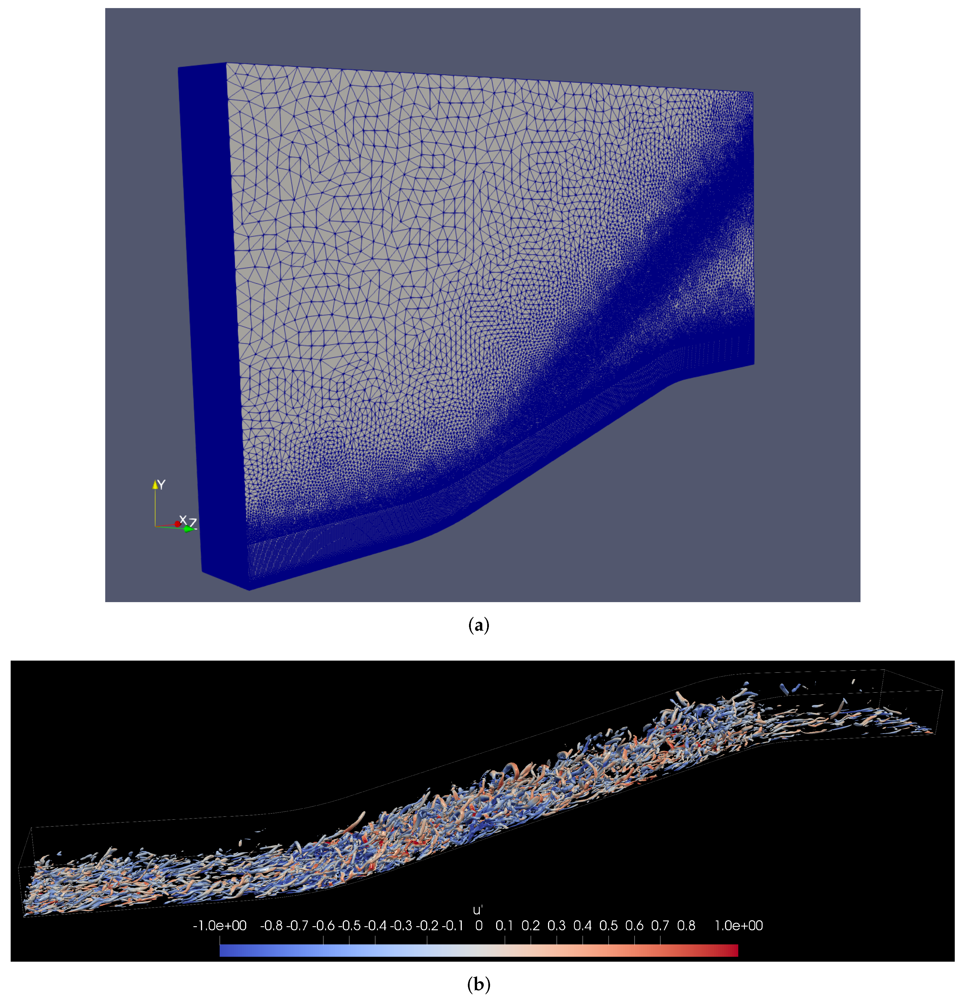
• The dataset employed in Stampede2 consists of 792 flow fields of the supersonic concave-convex DNS [45]. The hybrid unstructured mesh consists of approximately 9.9 M cells and 8.5 M points, as seen in Figure 3a. Note the inclined source region of pyramid elements (five faces) to capture better the compression waves generated by the concave-curved wall. This inclination angle (≈35${}^{\circ }$) was obtained by previously performing a 2D RANS analysis in concave walls [46]. The turbulent inflow conditions were prescribed based on a Zero-Pressure Gradient (ZPG) case, or turbulence precursor [47], Ref. [48] via DNS. The uncompressed size of the dataset is approximately 150 GB using double precision and stored in HDF5. The mesh contains roughly 5 M nodes (565 × 80 × 105 along the streamwise, wall-normal, and spanwise direction, respectively) just in the structured part with hexahedra. We visualize regions where $Q>0$ colored by the instantaneous streamwise velocity fluctuations, $u^{\prime }$, normalized by the freestream velocity in Figure 3b based on the Q-criterion. The rotational nature of the flow is enhanced due to the concave wall’s adverse pressure gradient. Further, more complex structures such as hairpin-like vortices can be seen throughout the ramp. In general, the legs of hairpin vortices show negative values of $u^{\prime }$, whereas the hairpin vortex’s heads exhibit positive values of velocity fluctuations. Again, we stored pressure, temperature, and velocity components for each node. The lower storage footprint for the Stampede2 benchmark is due to the available node hours.
• The datasets employed in Narwhal stress two areas of our proposed library. The first dataset explores strong scaling for a relatively low operation count over a large dataset (∼4160 GB), and the second dataset explores strong scaling for a higher operation count (more intermediate structures and operations) over a smaller dataset (∼380 GB). For the larger dataset, we compute 40 two-point correlations with 21 planes smoothing, which totals 840 intermediate TPCs with only 40 intermediate structures and TPC function calls per flow field, five energy spectra, and 25 cross-correlations on this dataset, which consists of 2001 flow fields of a High Reynolds number ZPG boundary layer. For the smaller dataset, we compute 315 two-point correlations with a nine plane smoothing, which totals 2835 intermediate two-point correlations with 315 intermediate structures and TPC function calls per flow field, five energy spectra, and 25 cross-correlations on this dataset which consists of a larger sample of the Stampede 2 dataset (2001 flow fields). In addition, we introduced a second dataset to explore the effects of the pre-fetcher on a similarly large dataset (∼3380 GB) composed of 20 times more flow fields, with each flow field being roughly ten times smaller (40,000 flow fields). This dataset is also from a Direct Numerical Simulation (DNS), albeit at a lower Reynolds number [44]. With this secondary dataset, we explored the impact of pre-fetching on data that would not stress the compute elements as much as the High Reynolds dataset; thus, we turned the weight towards a more latency-sensitive portion where reading times could bottleneck the efficiency of the compute kernels. We performed 30 TPCs, 26,400 energy spectra, and 25 cross-correlations for this secondary dataset.

3.5. Benchmark

The compulsory out-of-core read requirement for the benchmark for Onyx and Copper is 1254 reads (two reads per timestep). The first pass of the benchmark calculates the mean flow, which requires one complete access to the entire dataset. The second stage of the benchmark calculates the fluctuations, fluctuation RMS, the two-point correlation for $\mathcal{O}\left(10\right)$ wall-normal coordinates, and the cross-correlation between 5 variable pairs.

The benchmark for Stampede 2 used a pre-computed mean flow field. Thus, each flow field is read-only once, resulting in 792 compulsory reads. The benchmark computes 50 total 3D two-point correlations for each variable resulting in 250 whole-domain TPCs. It also calculates 250 energy spectra at each location (not the entire domain), 12 cross-correlations, and three auto-correlations. Contrary to the Onyx benchmark, which is formulated using dot products, the two-point correlations are implemented in matrix multiplications with a Toeplitz matrix.

3.6. Results in Copper

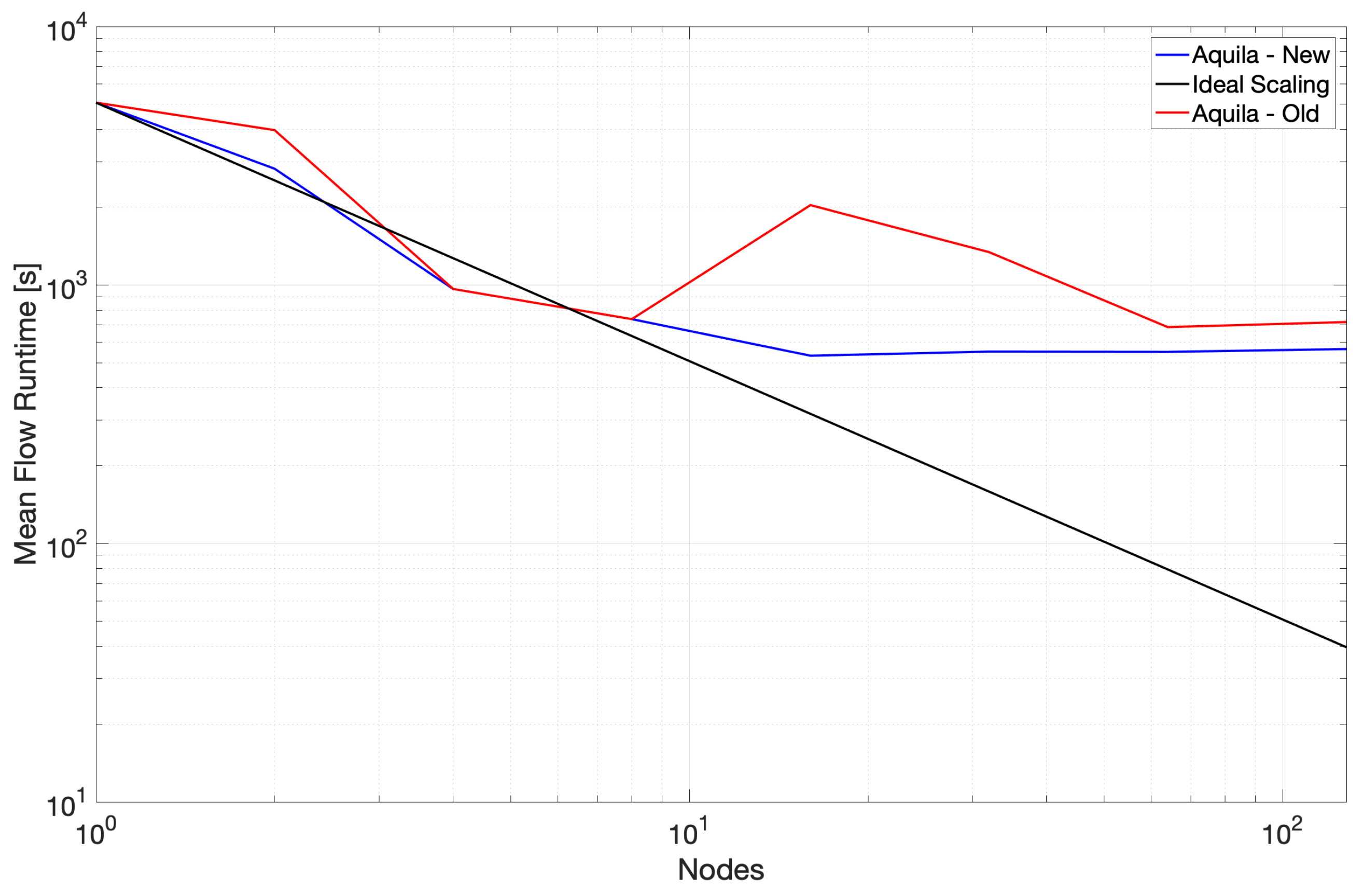
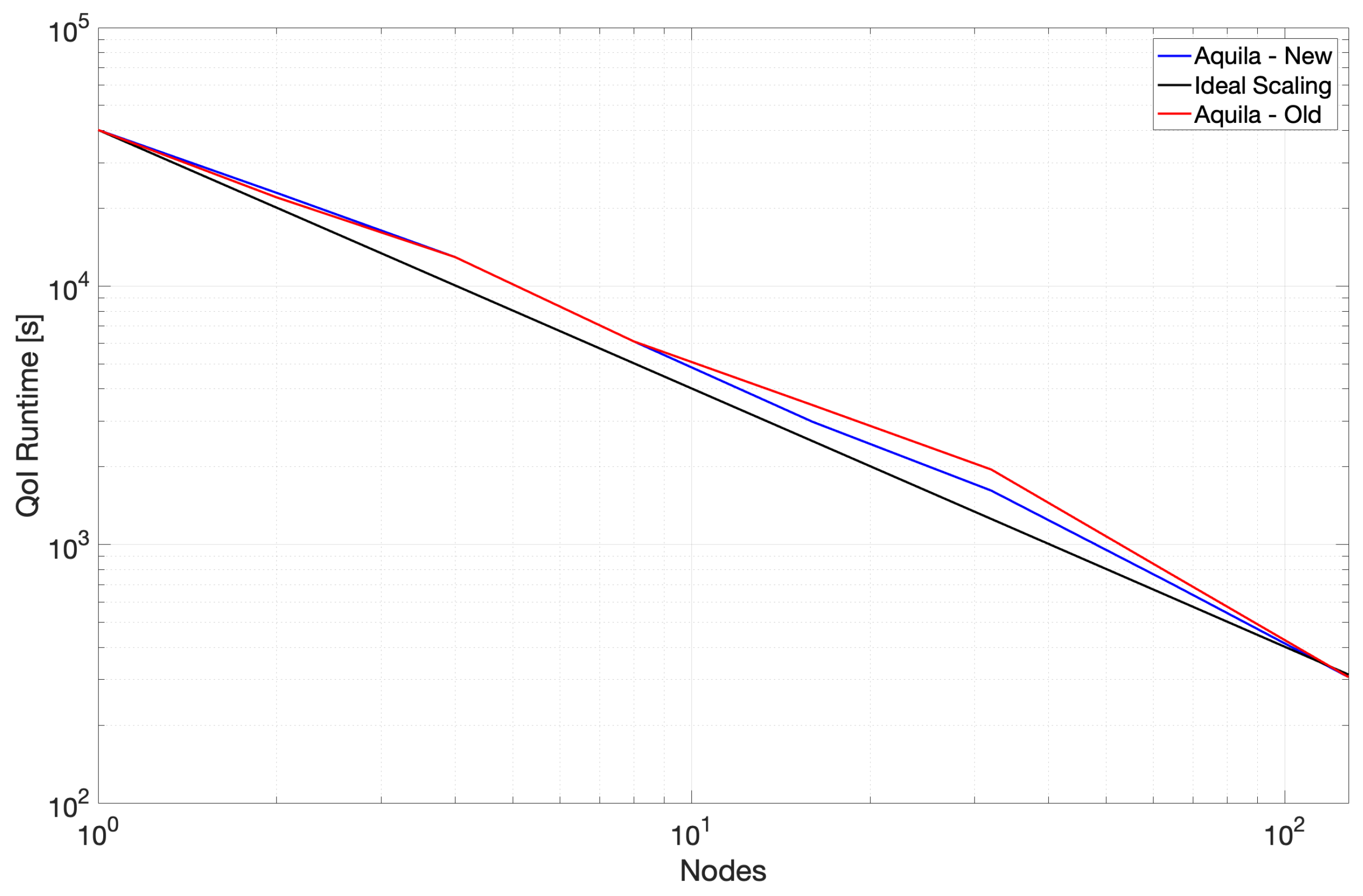
We present strong scaling data for two revisions of the Aquila C++ implementation (denoted Old and New in the figures for clarity). Old scaling data show results where vectorization was sub-optimal in some of the fundamental operations. We were unknowingly paying a high abstraction penalty [49,50] in the tight loops consuming the majority of the runtime (at the time, the 3D TPC). The Intel compiler could not optimize through multiple layers of abstraction, starting on the higher-level distributed volume class down to the Kokkos parallel loop abstractions. Noting that the generated x86 code was mostly scalar and had a few SSE instructions, we rewrote the TPC kernel using AVX2 intrinsics to assess the impact of the lack of vectorization (as mentioned in Section 2.3) and noted a dramatic performance improvement.

The critical lesson is always to verify code generation; this is especially true when higher level abstractions are invoked. The implementation became much more performant, and we did not lose maintainability. Upon verifying this performance gain, we unboxed the underlying data manually (i.e., get a raw pointer to the data on a confined code section), called the kernel directly on the data, and returned the boxed result. The pure Kokkos fallback path was still available when AVX was unavailable, or an unoptimized platform was encountered. We also tuned the build scripts to lower the vectorization threshold and allow more aggressive vectorization in other operations. For the most recent version of Aquila, the previously described minor updates reduced the abstraction penalty to the core implementation of these operations, which resulted in significant gains in overall application runtime (up to 2× improvement in overall application runtime, 2–5× reduction in runtime for mean flow calculation which is limited mainly by the latency of individual operations) and 25% peak for the remainder of the compute core which was already well-optimized and is more throughput-dependent rather than latency-oriented. The observed speedups are within the realm of the expected since scalar to AVX2 could yield a 4–8× depending on the precision being used, whereas SSE to AVX could theoretically deliver a 2× improvement. This serves to underscore the importance of leveraging all available parallelism and also the importance of separating low-level implementation for higher-level interfaces. For measuring low-level runtime statistics such as the application’s cache behavior, we used CrayPAT (version 6.2.2). For calculating runtime execution, we use timers embedded in the application to measure individual components.

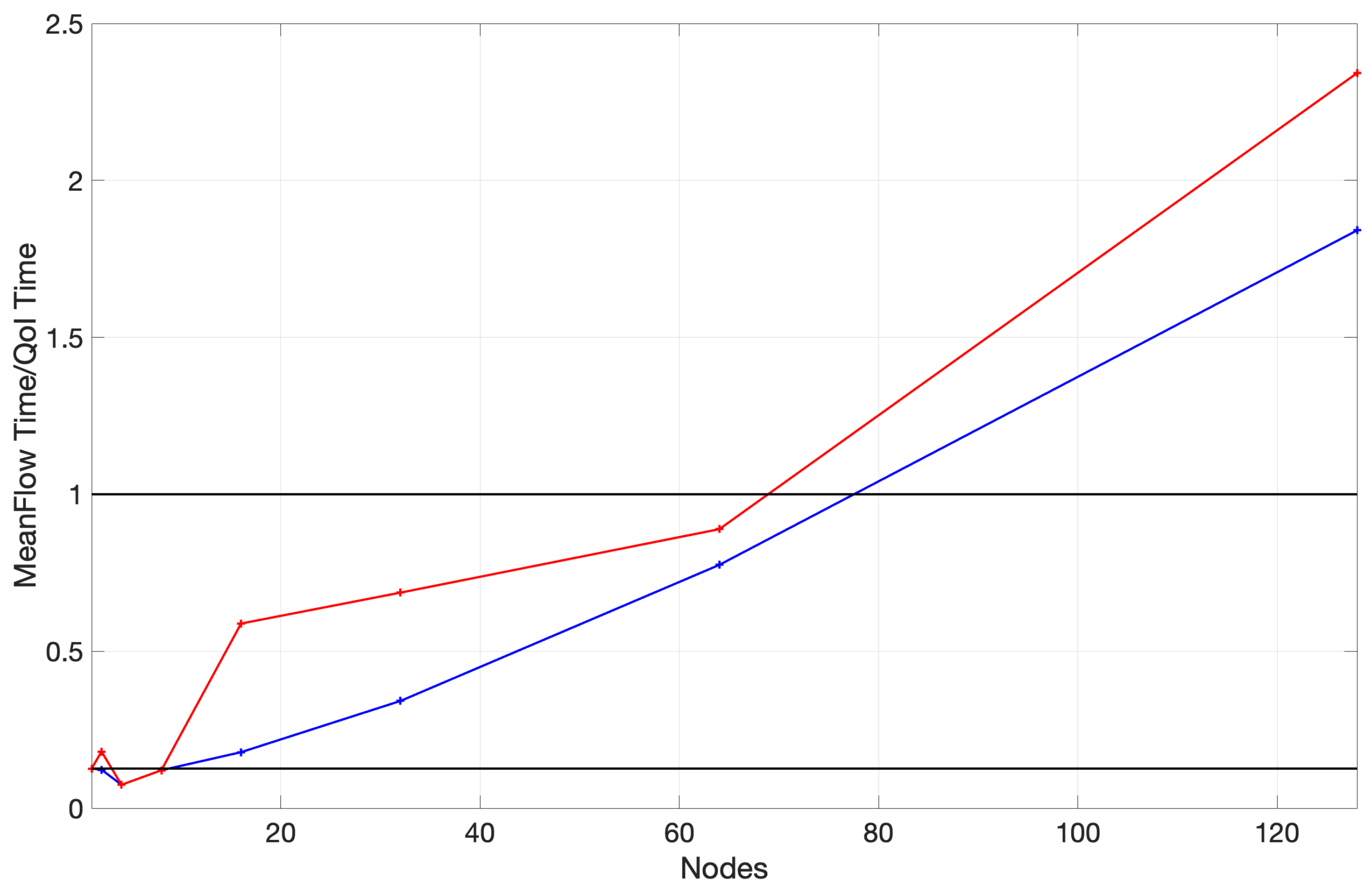
Aquila strives to maintain optimal serial performance. This leads to scaling potential by reducing serial bottlenecks. Part of this effort focuses on algorithms that are suitable for caching. CrayPAT reports about 96% L1D cache hits and 100% L2 cache hits every run. This is due to the cache awareness of the TBB pipeline and the optimized loop layout and memory allocation, which allows optimization of the CPU’s hardware pre-fetcher and speculative execution engine. Calculating the average flow rate becomes a critical path when the number of cores is significant, and it raises some research issues currently under investigation. On the one hand, the run-time ratio between the core and average flow calculations should ideally be constant (and significantly less than 1). A single pass through the data is indispensable for calculations requiring the mean flow, which we refer to as the core compute or quantities of interest. Thus, this first pass through the data is latency-bound as it is often limited by the IO fabric rather than the computational limits of the processor. Even with an efficient pre-fetcher, it is likely that the processor would have to wait for data to become ready since the mean flow essentially requires one multiply-accumulate instruction per mesh node per variable. In theory, this essential operation should scale very well with the number of nodes since more IO links become available. Contrary to this, this ratio grows monotonically, which can be likely attributed to several factors. These factors are reinforced by our results in Onyx to be discussed later in this paper, including:

• The lack of sufficient work to hide the fetching latency. This is often the technique used by massively parallel accelerators such as GPUs to hide the latency of memory accesses with additional independent work that can be concurrently scheduled on shared execution units.
• The flooding of the single Lustre MDT with requests. The Lustre filesystem has separate servers for metadata and the actual data storage layer. Although not inherent to Lustre, the metadata servers are often significantly outnumbered by the storage servers. This is perfectly reasonable since many HPC parallel filesystems expect large parallel workloads. However, this imbalance becomes notable to a user when many MPI ranks attempt to open or query metadata details of a large number of files simultaneously. The current Aquila design splits flow fields as independent work units to expose a large amount of embarrassingly parallel slack. Although this is often not an issue on many HPC systems, Copper had a single metadata server which could have hampered the scaling significantly. We verified this by moving to a system with multiple MDS and noted that this bottleneck was no longer present (see the next sections for more details).
• The amount of network fetches being made to a relatively small amount of OSTs. As previously outlined, the Lustre architecture separates the storage and serving of metadata from the actual data. The Object Storage Server (OSS) is backed by Object Storage Targets (OSTs) that contain the actual data in storage media (usually hard drives). A small number of OSTs with hard drives and large IO traffic can significantly degrade the performance since the spindles inside the drives have to search for the reading location constantly. Hard drives are notoriously bad at random IO, which is the pattern somewhat induced by many concurrent reads and writes to an underprovisioned Lustre filesystem.

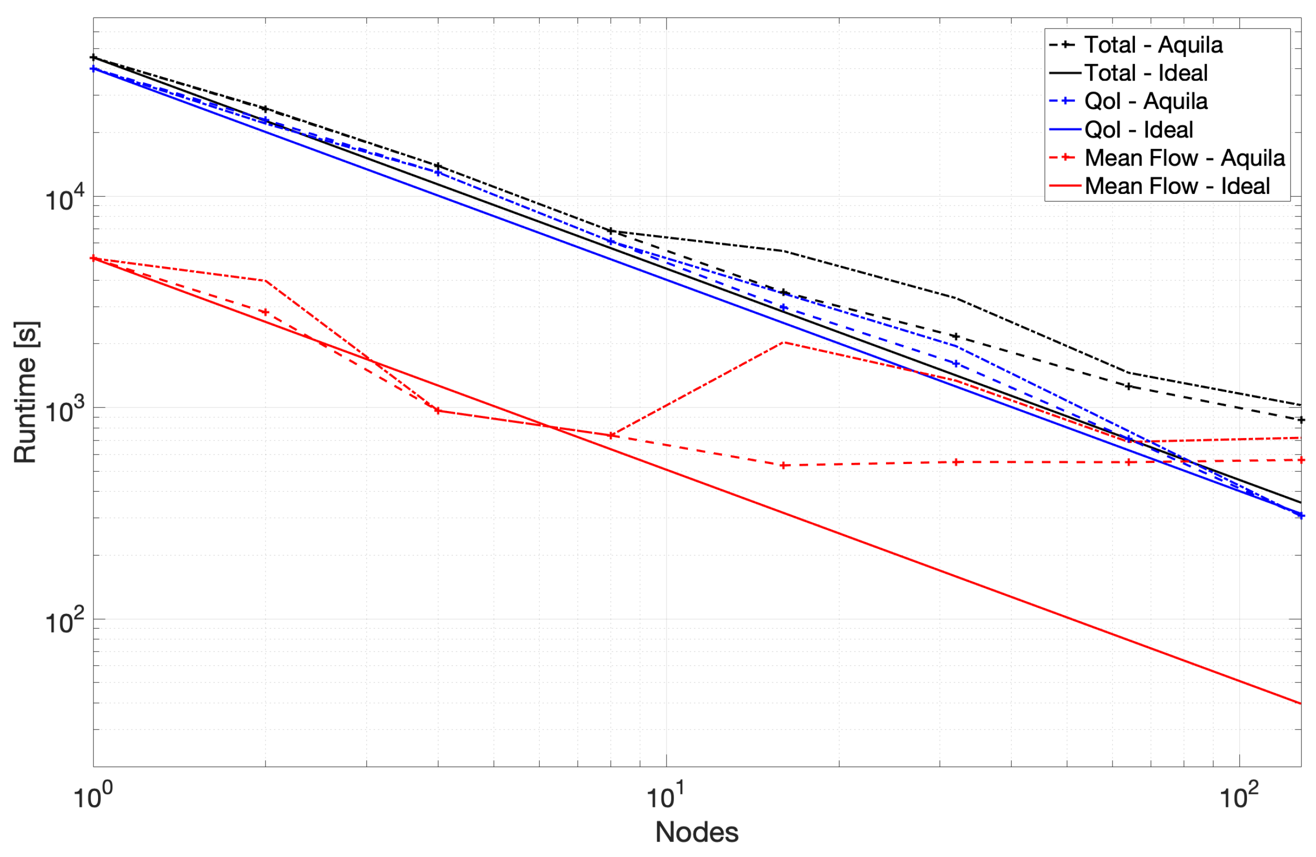
A bird’s eye view of the benchmark’s runtime is presented in Figure 4 to underscore the overhead of calculating the mean flow at higher numbers of nodes. It shows three distinct runtimes, including the mean flow’s calculation, other flow statistics, and an overhead which we define as the simple difference between the sum of the core runtime and the overall runtime. To enrich the visualization of these results, we also present the proportion of the time invested in the mean flow to the time required to generate all other flow statistics in Figure 5.

A notable improvement further reinforces the first of these observations in strong scaling at higher core counts achieved by reducing single-threaded runtime. This, in turn, reduces the latency and increases the overall throughput per unit time of individual flow fields proportionally (see Figure 6). A more balanced storage system is required to verify the remaining two observations. This being said, many parallel file systems exhibit performance degradation under high metadata queries along with competing reads.

The scaling performance for the second portion of the benchmark is considerably better with nearly linear scaling throughout the test and slightly super-linear scaling towards 128 nodes. We combine these results into a single plot to provide some context to the critical nature of the mean flow path at higher node counts and show the results in Figure 7. Removing the mean flow calculation from the benchmark yields a runtime remarkably similar to that presented in Figure 8.

A rudimentary solution for the issue caused by calculating the mean flow at very large core counts could be simplified by pre-calculating the mean at lower node counts and storing the result for use by a later job at higher node counts. Insufficient work could be the culprit of many scaling issues.

The parallel efficiency of the core portion of the compute benchmark is over 80% in all but a single outlier. The reason why the 32-node runs achieve under 80% efficiency is not apparent. Nonetheless, the scaling efficiency recovers at higher node counts. Leaving the anomaly in calculating the mean flow at higher node counts, Aquila exhibits near-perfect strong scaling for its core components. This remains true while operating out-of-core with data stored in hard drives and connected over the network. With the growing size of numerical simulations, it is possible that even single timestep data could not fit within a single node alongside other intermediate memory buffers. To this end, out-of-core data are becoming worth considering when developing scientific applications hoping to be resilient in the future.

3.7. Results in Onyx

We also verified the single-core performance of a more modern CPU architecture, Intel Broadwell, on the Onyx supercomputer, which alleviates some of Copper’s limitations by increasing the number of available OSTs, MDTs and using the Dragonfly topology on the Cray-Aries network. Preliminary data suggest that the current method can take full advantage of modern hardware with a simple recompilation. For example, after Onyx recompiled Aquila for Intel Broadwell, the runtime was reduced by 3.4× (peak), which is likely a trend toward improving hardware in the rapidly evolving computing world. On the most extensive run of Onyx, we also achieved a minimum run time of 2 minutes.

Distributed Performance

Onyx is a more balanced system, which is reflected in the results shown in this section. Up to 1200 nodes (105,600 threads) maintain nearly 100% parallel efficiency. At 2400 nodes (211,200 threads), it drops to around 80% in Figure 9. This is remarkable considering the nature of Aquila’s out-of-core, pipelined asynchronous data pre-fetching. As processing power and network performance grew, we introduced the concept of reference points to take advantage of homogeneity and quasi-homogeneity. Since periodic boundary conditions are specified along the spanwise direction, spanwise uniformity can be safely assumed. Additionally, Aquila allows you to set additional reference stations at compile time. This can be used for local quasi-uniform flow at various points in the flow direction. The previous numerical toolchain took more than two months to process 249 reference stations (excluding span stations). We ran a benchmark on Onyx and used 52,290 two-point correlations for each regular wall station. However, it represents an atypical form of scaling research. We set the number of nodes to 600, increase the number of reference stations, evaluate the impact on runtime, and display the results in Figure 10. More computing work for each loaded file improves resource utilization by improving hiding delays. The proposed approach thrives when the pre-fetcher and network performance enable latency hiding, similarly to GPUs when swapping groups of threads to hide fetching latency.

Figure 11 shows Aquila’s scaling from just ten nodes to 2400 nodes with excellent parallel efficiency (crucial to efficient resource utilization in large-scale computers). Furthermore, small cases run efficiently, even on laptops (although results for these are not presented). This is crucial for efficient use as we can post-process results where it is more appropriate rather than turning everything into a nail once the hammer is available.

3.8. Influence of Memory Allocator

Further, we have also examined the application’s pliability by varying the memory allocator. We tried this by substituting the compiler-default allocator invoked at runtime by the Intel TBB Scalable Allocator, which improved cache behavior. We replaced the allocator using the dynamic library pre-loading approach provided by TBB. We noticed a further reduction in the runtime of roughly 1–2%. The impact, although relatively small, is measurable, and slight decreases add up over time. The effect would likely be more significant at higher SMT modes in the future, where greater contention for the allocator is much more likely.

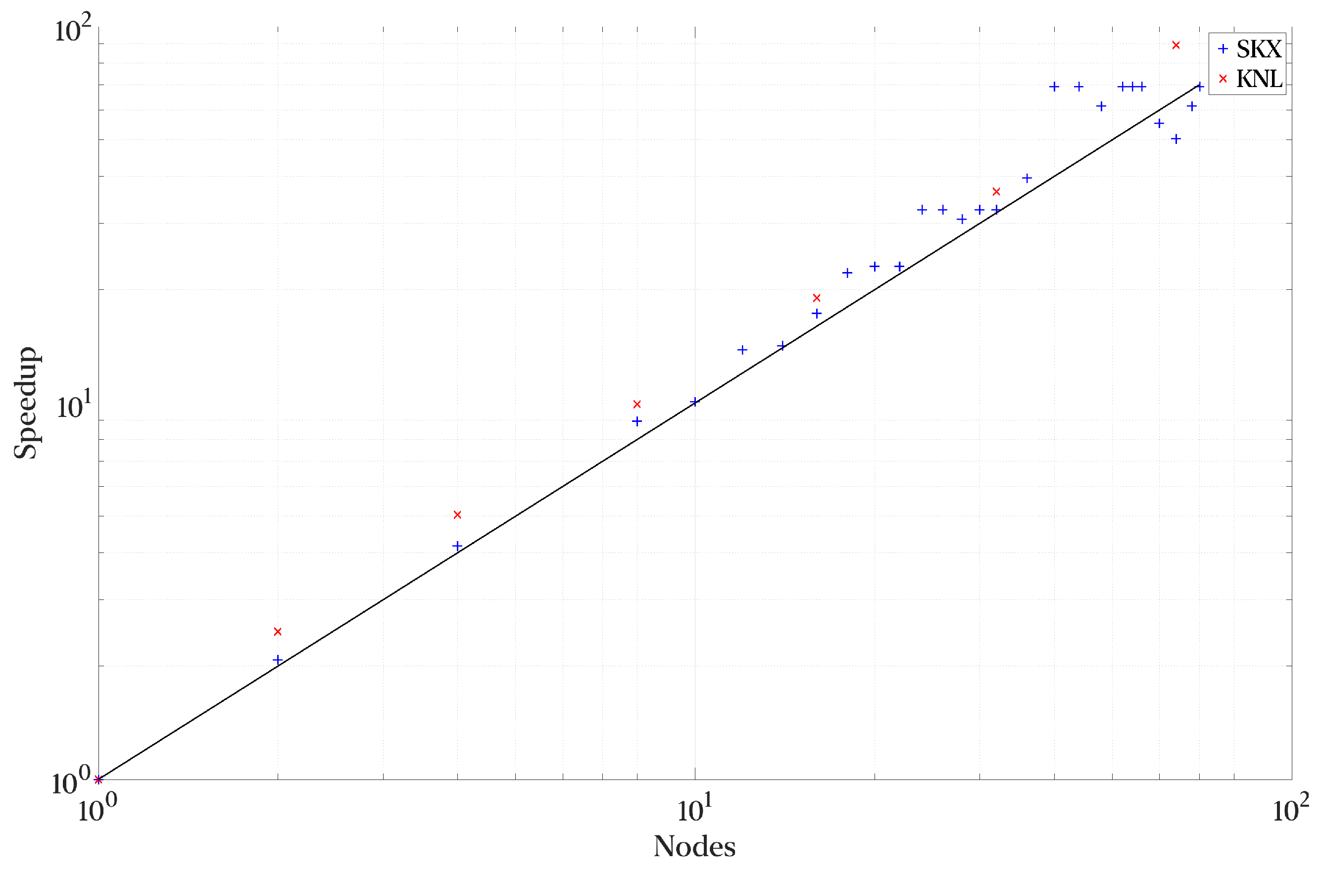
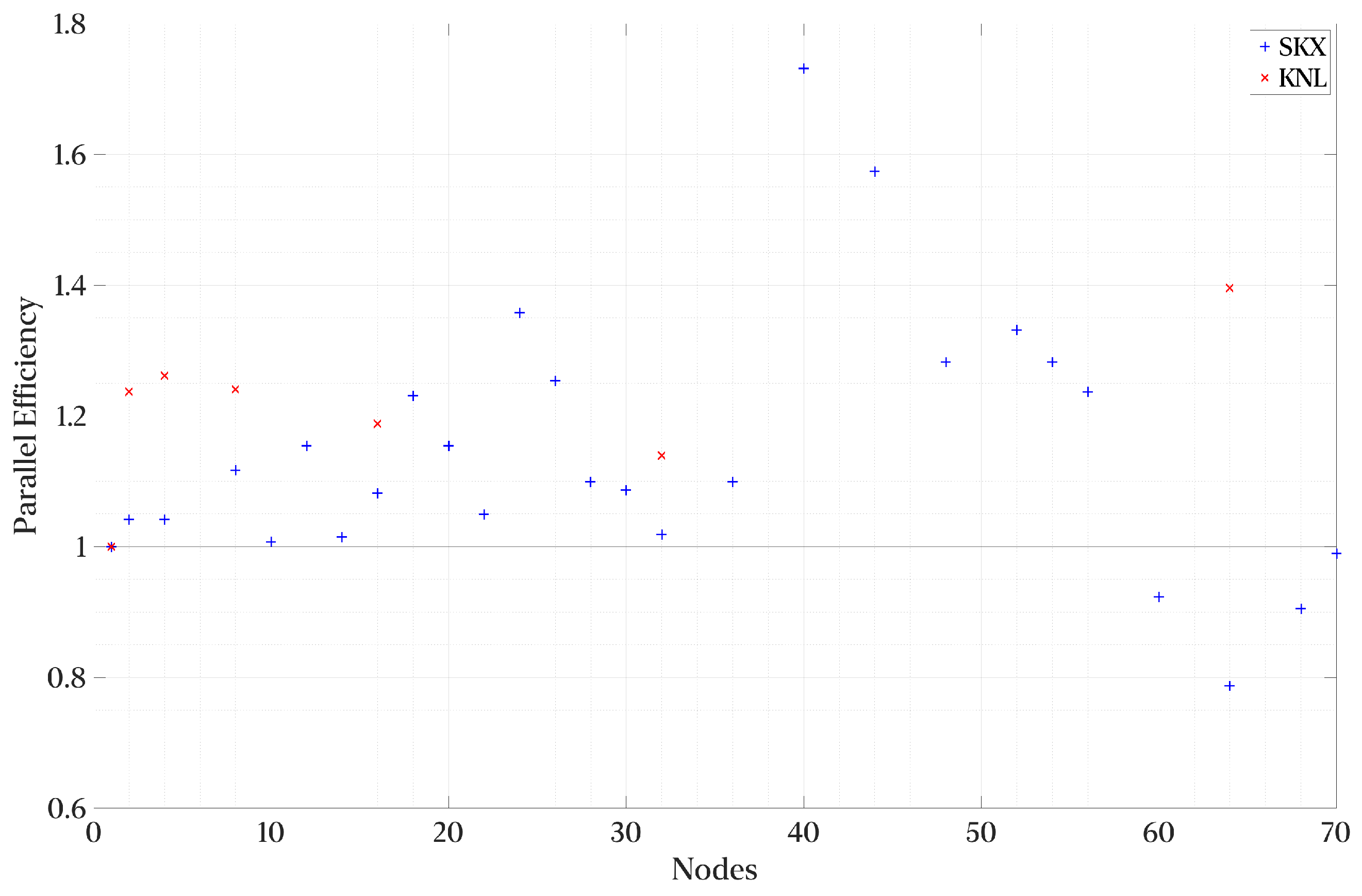
3.9. Results in Stampede 2

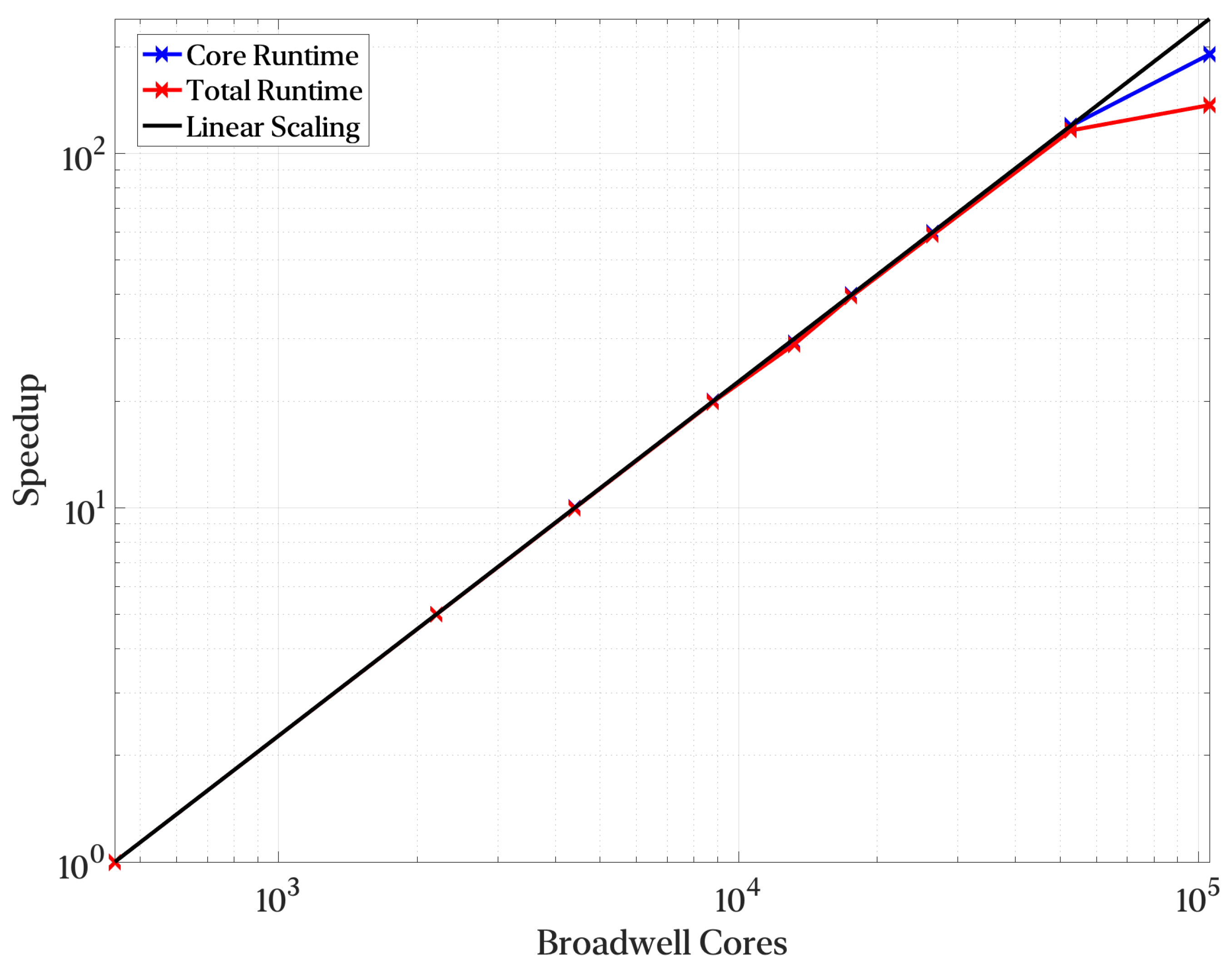
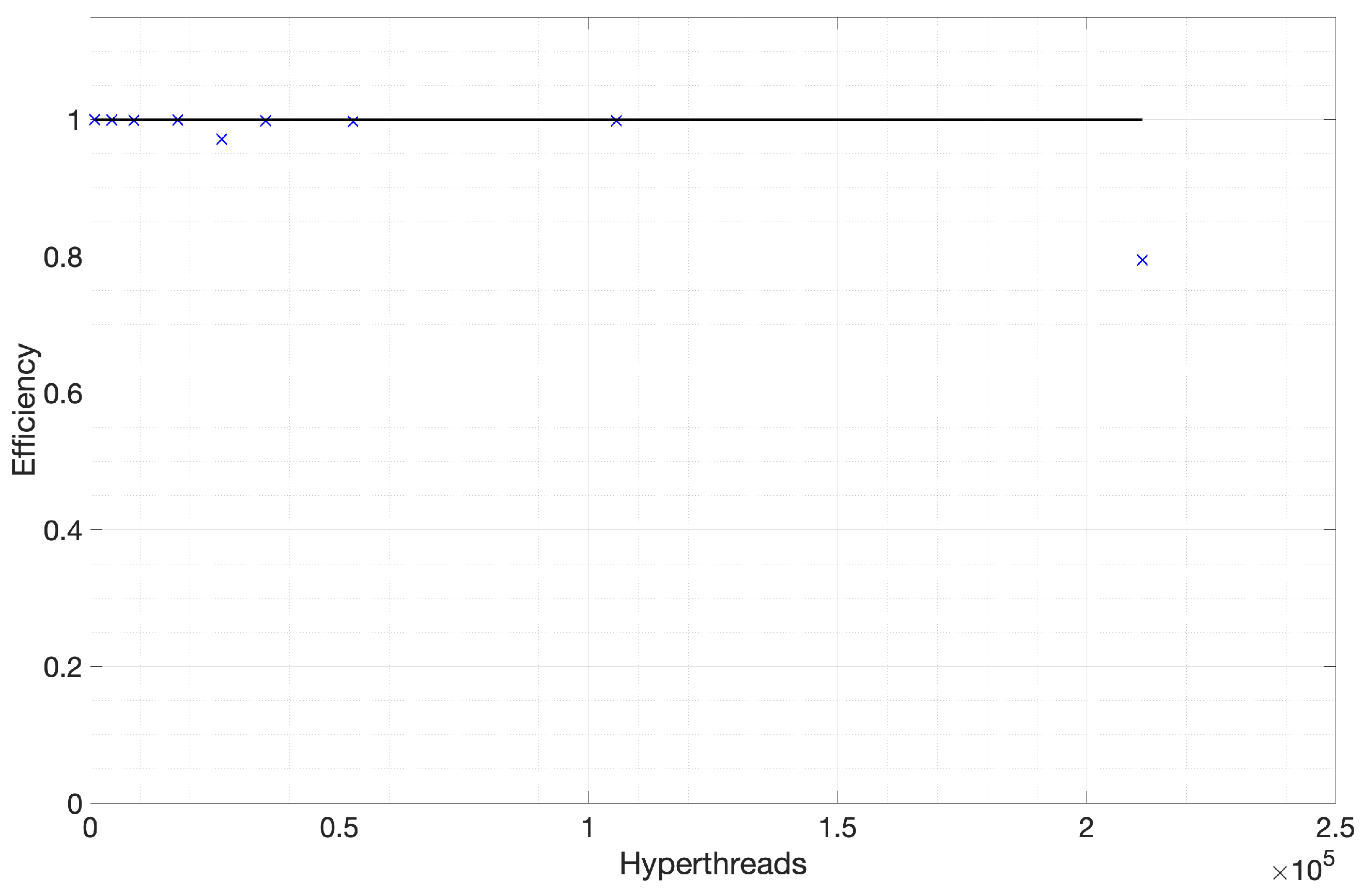
Figure 12 and Figure 13 show the strong scaling performance and parallel efficiency of the Python implementation at the Stampede 2 cluster discussed in Section 3.2. Overall, we observe super-linear scaling and efficiency. A simple explanation for this behavior is the network load by full flow field reads. A typical NIC in a node has 2–4 ports, and 8–11 workers per node compete for these ports. By adding additional nodes, we tap into the greater capabilities of the interconnect and IO connections. On average, the parallel efficiency is around 115%.

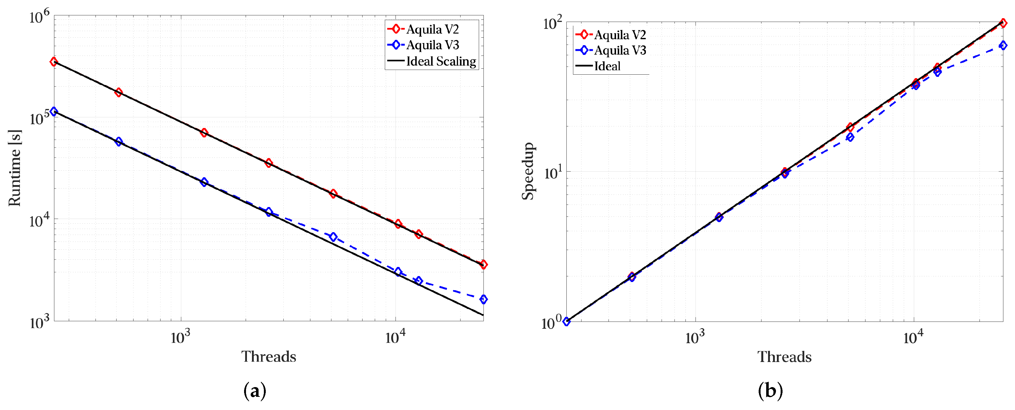
3.10. Results in Narwhal

As was previously mentioned, we employed a larger dataset to assess strong scaling over a reduced number of operations applied to a multi-terabyte dataset. The results for the larger dataset are presented in Figure 14. We see that including an asynchronous engine for operation scheduling results in a 2–3× speedup over a linear scheduling engine where each operation is parallel internally. This is due to better utilization of the 256 threads per node. The smaller dataset was used to stress the total number of “in-flight” operations and intermediate structures. The introduction of a thread pool with a dynamic work partitioning as the one in TBB does yield a worsening of strong scaling at higher node counts of roughly 20%. This has been confirmed over three trials. Recovering this strong scaling is currently the subject of further research.

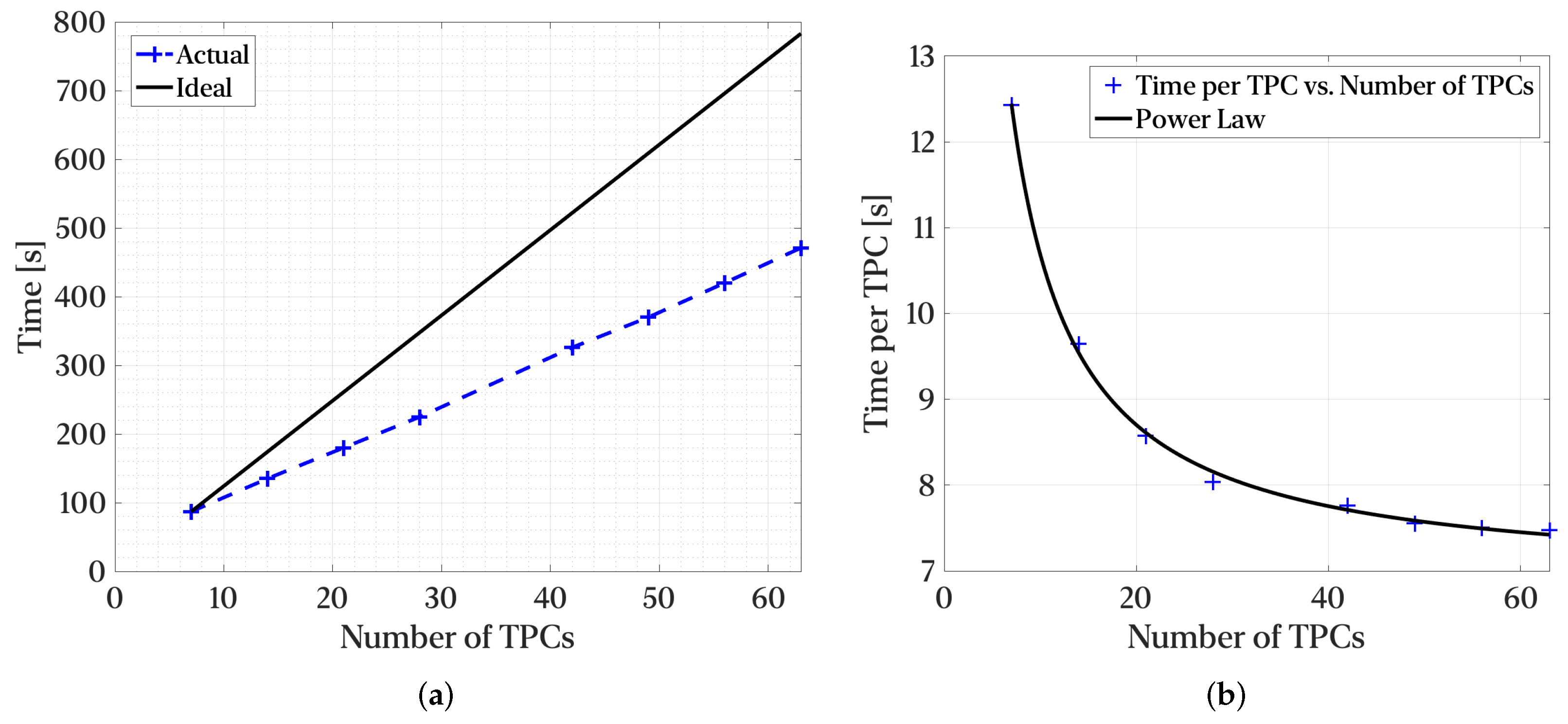
As scientific needs tend to grow over time, with additional statistics typically required to enable richer analysis, the number of calculations grows. To simulate such scenarios, we limited the size of the dataset to stress latency requirements and linearly varied the number of two-point correlations from 7 per variable (5 flow variables) to 63 per variable. The number of intermediate TPCs generated for smoothing grows linearly from 315 to 2835. The results are presented in Figure 15. The total compute time grows sub-linearly, indicating that the computational requirements grow less aggressively as scientific needs grow. The power-law presented in Figure 15b has an offset of 6.5 s and an exponent of −1.07. The V2.1 implementation can also reach 64.4% of peak memory bandwidth on a single node, which is remarkable for an out-of-core application.

3.11. Impact of the Asynchronous Pre-Fetcher

As part of our scaling study in Narwhal (see Section 3.3), we conducted a survey replacing the pre-fetching operations in Aquila with a blocking call to the reading function. This allowed for an “apples to apples” comparison and an impact on program runtime as directly related to non-blocking, pre-fetched reads. We found the effect of the pre-fetcher to be directly related to the size of the data. As previously mentioned, we included a secondary dataset that would be more sensitive to read times in addition to the primary dataset that included larger flow fields. For the higher Reynolds data (i.e., the larger dataset), using non-blocking, pre-fetched reads reduced the program runtime by 21% (the calculation for the mean flow was accelerated by 13% whereas the remainder of the calculations exhibited a 23% reduction in runtime). The lower Reynolds dataset showed a 35% speedup using the asynchronous pre-fetcher (similarly, 23% in the mean flow calculation runtime and 46% in the core portion of the benchmark). Thus, depending on the workflow, dataset size, and the number of calculations required, the asynchronous, pre-fetch mechanism allows for 20–35% total runtime reduction with a reduction in more compute-intensive portions of the benchmark nearing 50%. This gives the “illusion” of an in-memory dataset being operated on by reducing drastically the idle time spent blocking on reads to a network-bound parallel filesystem common to many large-scale clusters and supercomputers. This is in line with the reported degradation of 29% for an optimized out-of-core application running off flash vs. memory reported in Figure 6 of [10]. This being said, Morozov and Peterka [10] reported a performance degradation for an optimized out-of-core application of up to 78%. In summary, the speed-up observed in the present work can be directly explained by simply allowing overlap of computation with an asynchronous data pre-fetcher; multi-terabyte datasets can be handled without paying the total cost of reading fragments of data when needed as this cost is effectively amortized.

3.12. General Remarks on Strong Scaling

In this section, details and comments on the excellent strong scaling obtained for the shown benchmarks are supplied, which is due in part to our decomposition strategy. Temporal decomposition turns most of the problem into an embarrassingly parallel problem since each flow field can move through the pipeline independently, and synchronization occurs only at the final reductions when time averaging occurs. A significant deterioration in strong scaling occurs when favoring spatial decomposition over temporal decomposition. This is a luxury affordable in this work since the simulation is completed and the library has access to all of the temporal data and can schedule work across independent flow fields. We allow each worker to operate independently without any synchronization and introduce collective reduction operations afterward, thus maximizing the amount of parallel slack. To provide context, temporal decomposition provides up to the number of flow fields in temporal workers. After that, only spatial decomposition can be introduced to allow for further scaling. Spatial decomposition is sometimes the only alternative when a flow field or intermediate structures would not fit into the shared memory of a process. To come to the point, a numerical post-processing problem can be transformed into an embarrassingly parallel problem by favoring independent, temporal decomposition with minimal synchronization among workers. This has yielded excellent strong scaling performance in the present work and the studied problem domain.

4. Application Results

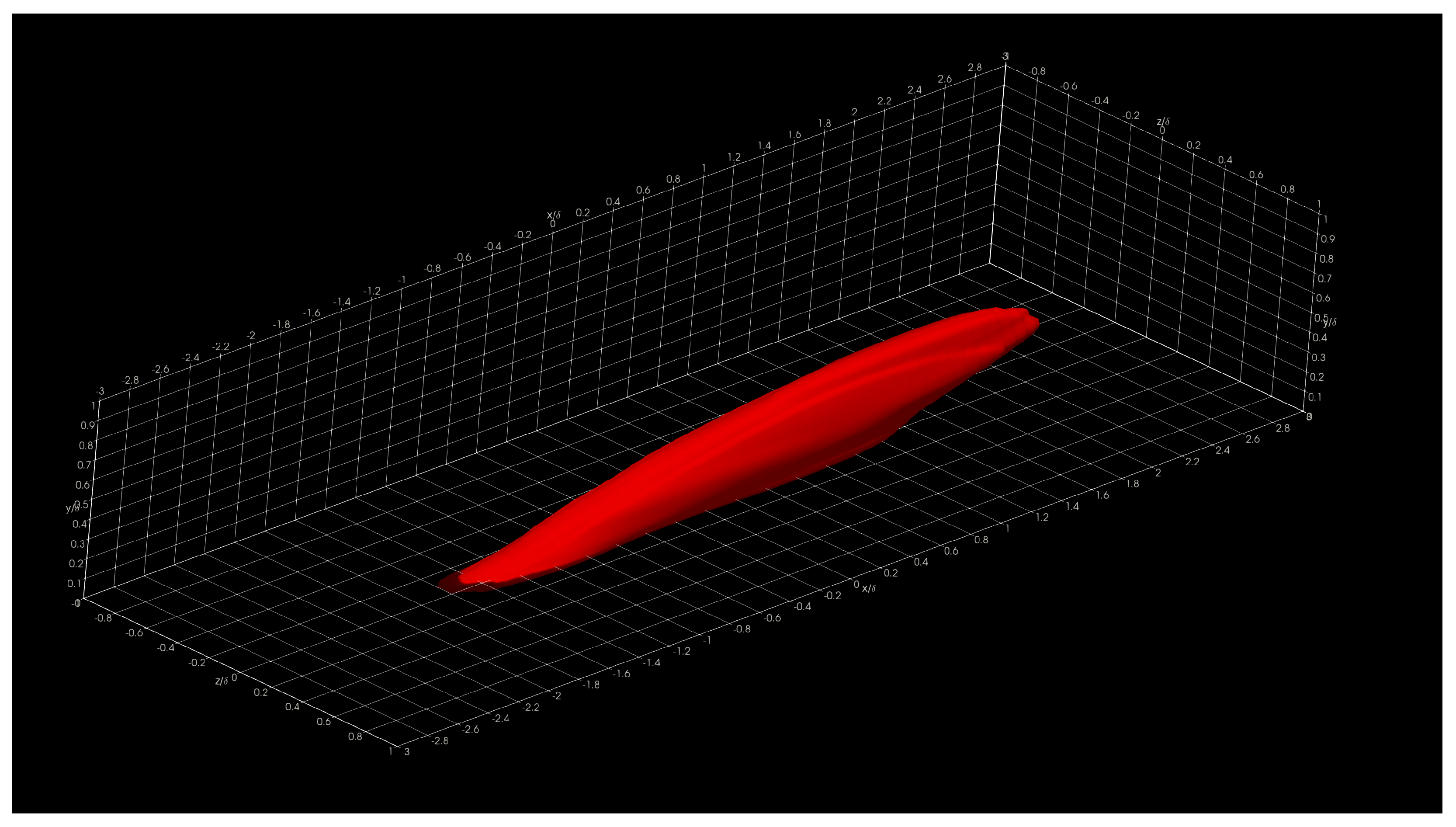
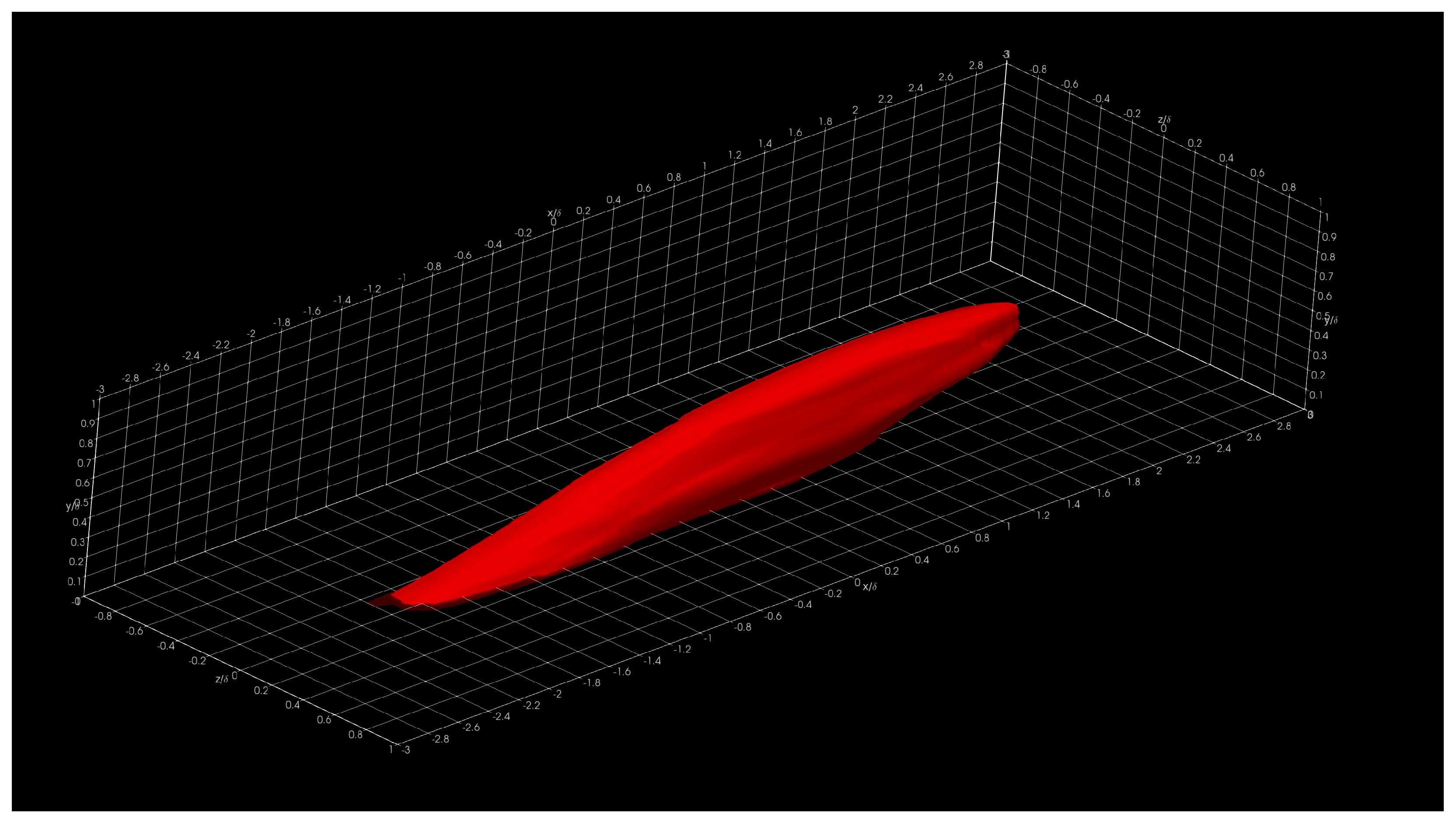
In this section, we show and discuss some results obtained using Aquila in the Onyx benchmark dataset. Specifically, we show three-dimensional two-point correlations (TPC) for the full supersonic High Reynolds number domain for the streamwise velocity fluctuations at $y^{+}$ = 5, 15, 50, and 100 in Figure 16, Figure 17, Figure 18 and Figure 19, respectively. Here, the superscript + indicates inner units in turbulence by dividing the wall normal coordinate, y, into the viscous length scale ${\nu }_w/u_{\tau }$. Here, ${\nu }_w$ is the wall kinematic viscosity and $u_{\tau }$ is the friction velocity defined as $\sqrt{{\tau }_w/\rho }$, where ${\tau }_w$ is the wall shear stress and $\rho$ is the local fluid density. Note that we present iso-surfaces of the two-point correlation function. The wall-normal coordinates $y^{+}$ were strategically selected in order to analyze coherent structures in the linear viscous layer ($y^{+}=$ 5), buffer layer ($y^{+}=$ 15), beginning and middle of the log region ($y^{+}=$ 50 and 100, respectively). The two-point correlation is emphasized and presented due to its computational intensity. On typical analysis, the calculation of the two-point correlation can account for 57–92% of the total runtime depending on the total number of reference locations.

The presented structures highlight the general nature of the Eulerian coherent structures as defined by the two-point correlation. In general, a coherent structure may be defined as that parcel of fluid where flow fluctuations are highly correlated, playing a pivotal role in the transport phenomena (mass, momentum, and energy) inside turbulent boundary layers. By extracting a specific threshold (usually 0.1 to 0.15; 0.15 for this particular showcase) of the normalized TPC function, one can infer that coherent structures exhibit an oblong “tilted” shape with long “tails”. The streamwise lengths of these turbulent structures vary from $2{\delta }^{\prime }s$ in the near-wall region to $3.5{\delta }^{\prime }s$ in the log region, where $\delta$ is the characteristic boundary layer thickness at the reference point or $x/\delta =0$. The influence (i.e., tails) of a downstream coherent structure over the near-wall region can be used to develop experimental turbulence characterization strategies since gathering velocity information near the wall under compressible flow conditions is often difficult at the very least. We have also observed more significant, coherent transport regions farther away from the wall extending towards the wall, illustrating the kinetic energy transfer across scales. Although not shown in the present manuscript, visualizing the two-point correlation also aids in assessing the Reynolds analogy by comparing the streamwise velocity TPC and the temperature TPC. Many other visual metaphors can be gathered by having a visual depiction of coherent transport regions and assessing flow isotropy.

Given the scope of this manuscript, we limit the discussion of the application results of coherent structure visualization via two-point correlation. However, we have presented a brief discussion. Interested readers are referred to [44,45,51,52,53] for further details about coherent turbulent structures discussions and other uses for the proposed post-processing library. The coherent structures present in the outer layer of the boundary layer are notably more prominent than those in regions closer to the wall (inner layer). From the visualization, we can readily observe the qualitative characteristics of the momentum transport. The visualizations include the viscous sub-layer, the buffer region, the log region, and the outer region of the boundary layer.

5. Related Work

The CFD Vision 2030 Study [54] outlined the need for scalable pre-and post-processing methodologies in addition to the actual simulation process as key to streamlining the whole computational pipeline and gathering detailed insights from large-scale simulations. Much effort has been poured into pre-processing by addressing high-performance mesh refinement tools such as AMReX [55]; highly efficient data storage methods such as HDF5 and pNetCDF [56,57]; and other pre-processing aspects. However, post-processing of large-scale simulations is often bounded by application-specific binary file formats, science goals, and other factors that limit creating more generalized, modular tools to gather insight from these numerical simulations.

At a high-level, computational fluid dynamics practitioners are faced with several post-processing alternatives, each with varying levels of complexity, versatility, flexibility, and customization options. Perhaps one of the best-known alternatives is ParaView [58]. ParaView is a fairly complex and comprehensive post-processing utility capable of visualizing large volumes of data in situ. However, ParaView is mostly focused on visualization and applying filters to mainly unstructured data. Given its generality, making domain-specific optimizations is generally impossible at the application level. This being said, Aquila does not aim to be a visualization tool. It aims to reduce the burden of calculating parameters inside a visualization toolkit and allows the visualization software to shine where it ought to. Similar remarks can be made with respect to similarly popular visualization frameworks that include FieldView [59], Tecplot 360 [60], and Ensight [61]. Nonetheless, all of these popular software packages are focused on data visualization and not on enabling simple and scalable calculations of complex quantities across enormous datasets and both CPUs and GPUs.

On the other extreme, more general libraries focused on out-of-core computations lack domain-specific optimizations and structuring that lead to the highly scalable performance demonstrated in this work. For instance, we previously showed that work by Morozov and Peterka [10] as a more general out-of-core computation library enabled expressiveness but had a significant performance loss when operating off the flash as compared to an in-memory baseline. Dask [62,63] is another popular out-of-core data processing library, but implementing certain fine-grained operations using Dask is not straightforward. In addition, Dask’s flexibility and generality make it attractive to many but hinder its full potential for domain-specific tasks. For instance, Khoshlessan et al. evaluated the use of Dask to post-process large-scale Molecular Dynamics simulations [64] and found intra-node strong scaling to be good but degraded as soon as multiple nodes were in use due to spurious occurrences of stragglers common in irregular, complex workloads. More recently, Legate Numpy [65] was introduced as a potential drop-in replacement for the famous [36] library with capabilities to automatically distribute work and data across workers in a cluster, including CPUs and GPUs. Although Legate Numpy seems like a potential candidate to implement much of the functionality seen in Aquila, installing and using it is not as straightforward and intuitive to practitioners used to the traditional MPI workflow since the default distributed memory library for Aquila is MPI.

To the authors’ best knowledge, there is no published work addressing scalable CFD post-processing tailored for unsteady three-dimensional numerical simulations with high spatial/temporal resolution (for instance, in DNS of compressible turbulent boundary layers). The proposed approach exploits domain-specific knowledge to optimize post-processing algorithms and introduce a modular pipeline independent of file formats. Furthermore, the proposed method leverages existing libraries standard to (or easily installable at) most modern HPC deployments, such as MPI, HDF5, C++, and Python.

6. Conclusions

This manuscript presents an overview of an out-of-core, performance-portable, and distributed post-processing library for large-scale computational fluid dynamics. Given sufficient work, we have included strong linear scaling results while operating on data stored in hard drives. We have also discussed the importance of guaranteeing platform-agnostic abstractions enabling applications to target existing heterogeneous computational environments and those to come. We have also shown that insufficient work could significantly degrade performance in out-of-core applications due to increased difficulty in hiding latency. We have also highlighted the benefits of providing additional information to the compiler to facilitate vectorization.

Further, we demonstrated parallel efficiency above 70%, and our most recent implementation achieves 50–60% of peak CPU memory bandwidth and 98% of the achievable filesystem bandwidth while operating out of the core. This strong scaling performance is notable as other attempts at out-of-core compute typically do not scale. We have also demonstrated the magnitude of the potential gains achievable by exploiting natural symmetry in a given domain in compute kernels. Among the main contributions outlined in this work, we have demonstrated that replacing blocking reads with asynchronous data pre-fetching can reduce runtime by up to 35% with some portions of the benchmark experiencing speedups of 46%. In addition, our approach is domain-specific to some extent which can be both a strength and a weakness compared to other out-of-core processing libraries. Further, the relevance of combining task and data parallelism on modern compute infrastructure was highlighted by a 3× performance improvement when enabling this combination in the core compute pipeline.