Genetic-Algorithm-Inspired Difficulty Adjustment for Proof-of-Work Blockchains

Abstract

In blockchains, the principle of proof-of-work (PoW) is used to compute a complex mathematical problem. The computation complexity is governed by the difficulty, adjusted periodically to control the rate at which new blocks are created. The network hash rate determines this, a phenomenon of symmetry, as the difficulty also increases when the hash rate increases. If the hash rate grows or declines exponentially, the block creation interval cannot be maintained. A genetic algorithm (GA) is proposed as an additional mechanism to the existing difficulty adjustment algorithm for optimizing the blockchain parameters. The study was conducted with four scenarios in mind, including a default scenario that simulates a regular blockchain. All the scenarios with the GA were able to achieve a lower standard deviation of the average block time and difficulty compared to the default blockchain network without GA. The scenario of a fixed difficulty adjustment interval with GA was able to reduce the standard deviation of the average block time by 80.1%, from 497.1 to 98.9, and achieved a moderate median block propagation time of 6.81 s and a stale block rate of 6.67%.

1. Introduction

The first prominent application in this field was conceptualized in a paper published by a pseudonymous author, or authors, named Satoshi Nakamoto. The paper is titled “A peer-to-peer electronic cash system” [1] and it proposed a framework for a decentralized electronic currency called Bitcoin. The framework actualized the research that was previously proposed by Haber and Stornetta [2], and was then coupled with a patent on the Merkle tree [3]. It was then implemented and proven to be a workable decentralized electronic currency that is immutable with limited circulation, similar to a sovereign-backed currency but without a centralized authority.

The core of the decentralization is the method for validating each transaction, where anyone can contribute processing resources to assist in validating the transactions in the electronic currency network. As it is decentralized, the process requires consensus between the nodes (miners) that are validating the transactions. The overall process is called proof-of-work (PoW) [4]. To obtain the consensus, the Bitcoin network conducts voting among the miners approximately every 10 min on the state of the Bitcoin network, to consolidate the validated transactions into a block (block time). In order to maintain the period between voting, that is the 10 min interval or the block time, the miners agree among themselves to adjust a variable called the difficulty, which is directly related to the overall computational resources that are available in the Bitcoin network. With more computational resources, the difficulty is set higher, and with less, it is set lower.

Bitcoin has grown in worldwide acceptance, and since its introduction, other electronic currencies (cryptocurrencies) have emerged. As the miners are rewarded for their effort in solving a mathematical puzzle (mining), the miners will tend to provide their computation resources to the most profitable cryptocurrency. This causes “coin-hopping”, where miners switch to the more profitable cryptocurrency [5]. As the miners switch their resources to mine a different cryptocurrency, the cryptocurrency they departed from will still have the same difficulty settings, until the next consensus is conducted. This can cause an issue with attempting to maintain the block time, due to a lack of computation resources for mining with high difficulty settings. Bitcoin’s difficulty adjustment algorithm is therefore susceptible to this drawback [6].

In PoW blockchains, the phenomenon of symmetry is observed, as difficulty also increases when the hash rate increases [7]. The block time can only be maintained by the difficulty adjustment algorithm if the overall computation resources (known as the hash rate) are constant. In the event of an increase in hash rate, the block time decreases and is adjusted through a retargeting mechanism regarding the difficulty, to maintain this equilibrium. However, as the retargeting takes place only after 2016 blocks in Bitcoin, the equilibrium is not maintained for a considerable length of time. Further, the network is not able to retain the block time if the hash rate rises or falls exponentially. In this paper, a genetic algorithm (GA) is introduced into the difficulty adjustment protocol to reduce the effect of the symmetry of the hash rate on the block time due to fluctuating hash rates in the Bitcoin network.

Proof-of-Work (PoW)

Dywork and Noar introduced PoW as a concept to address the issue of junk mail and administering access to shared resources [8], but the term “proof-of-work” was conceived by Jakobsson and Juels [9]. In order to access a shared resource, a feasible function that is reasonably hard must be computed as a requirement, and this serves to fend off malicious utilization of the shared resource.

Bitcoin implements PoW to provide resilience and security. A PoW process known as “mining” creates new Bitcoins, where the user or “miner” attempts to find a solution for a mathematical problem (PoW algorithm) through a particular piece of software. The target (T) is the threshold set for the block hash computed (to be less than) by the miner, for the candidate block to be valid. The difficulty (D) is a metric that indicates how hard it is to find a hash that is smaller than a specific target. As it is difficult to discover a block hash that is smaller than an already tiny value, a lower T will result in a larger D.

The new target, $T_{i+1}$, is calculated by multiplying T by the actual time it took to mine 2016 blocks and dividing it by the expected time, which is 20,160 min, as shown by the following equation [10]:

$$T_{i+1}=T\ast \frac{{\sum }_{i=1}^{2016}{X}_i}{20160\min }$$

(1)

where D is calculated by multiplying the target of the genesis block ($g_T$) with the current target ($c_T$), given by

$$D=\frac{g_T}{c_T}$$

(2)

The block time (B), which is the expected time taken to mine a block in Bitcoin, is approximately 10 min. A retargeting mechanism will automatically and independently ensure that the block time B is as close as possible to the expected 10 min [4]. In this case, T is periodically and dynamically adjusted to meet the expected B of 10 min. Whenever the block time falls below 10 min due to an increasing hash rate, T is lowered (increasing the difficulty) during the adjustment, and vice versa. In addition, a limit is also imposed on the adjustment to prevent drastic changes to D, as shown in Algorithm 1.

However, PoW does not respond or react well when the hash rate experiences sudden changes. This was evident in some blockchain networks where a rapid shift in hash rate was experienced when capable powerful mining hardware for other networks was repurposed specifically for these networks. Since Bitcoin only retargets once every 2016 blocks (approximately 2 weeks), mining is performed at an extremely slow pace until the next retargeting event occurs, when enough blocks are created. The difficulty adjustment algorithm acts as a feedback controller, where the difficulty is the input, and it is manipulated towards the desired block time based on the actual time taken to mine a block (measured output). This reactive approach has a few vital shortcomings [11]:

• The difficulty adjustment may overshoot or undershoot, thus causing the block time to oscillate significantly.
• Cryptocurrencies are susceptible to “coin-hopping” or “pool-hopping” attacks, where miners choose to only mine a specific cryptocurrency when it is profitable, and switch to another when it is not.

As a means of mitigating these issues, a GA is introduced into the difficulty adjustment protocol to regulate the variation of the parameters (i.e., block time, retargeting interval, etc.). We show that it is possible to achieve a more dynamic retargeting mechanism that is able to meet the network objectives.

Algorithm 1 Target adjustment limit

Set targetTimeSpan = expected time taken to mine a block (s) × difficulty readjustment interval Set totalInterval = actual time taken to mine N blocks iftotalInterval < targetTimeSpan then     totalInterval = targetTimeSpan / 4 end if iftotalInterval > targetTimeSpan then     totalInterval = targetTimeSpan × 4 end if

2. Literature Review

Several approaches have been introduced to improve the difficulty adjustment protocol, and in the process reduce the block time fluctuation. Bissias, Thibodeau and Levine proposed a proactive difficulty adjustment algorithm known as Bonded Mining (BM) in response to the relatively reactive nature of typical difficulty adjustment algorithms in PoW [11]. In BM, miners are required to commit to a hash rate which is financially bound to “bonds”, where the committed hash rate in turn adjusts the difficulty of the network. As the miners are bound to their commitments, they are required to follow through with them even when it is no longer profitable to do so. However, the commitments only last until the next block is created, and if the miners choose to “deviate from their commitment”, they suffer a fine that is equal to their divergence. In evaluating BM, block time stability simulations were carried out. The simulations compared the BM difficulty adjustment algorithm to the one used in Bitcoin Cash (BCH). The results showed that for BCH, the resulting block times diverged significantly from the intended time whenever the hash rate fluctuated, with the lowest block time reaching approximately 250 s and the highest reaching around 1500 s, with a recovery period of at least a day for the correction. Oscillation of the resulting block times was also observed, although the hash rate was maintained. With BM, a relatively lower amplitude in the oscillation and divergence of the block time was maintained, and no oscillation was observed when the hash rate was maintained, resulting in a block time that was closer to the intended block time.

Noda, Okumura and Hashimoto examined the behavior of the winning rate in place of the difficulty, and they found that the winning rate was “mathematically more traceable” [12]. Let W represent the winning rate, which is the probability that a block hash found by a miner is smaller than the target. H represents the hash rate, the total number of hash attempts per time unit. Based on observations, the average block time ($B^{\ast }$) can be calculated as $1/(W\times H)$. The winning rate can be adjusted to achieve a $B^{\ast }$ of 10 min. Noda et al. concluded that Bitcoin’s difficulty adjustment mechanism made it difficult to maintain steady block creation compared with Bitcoin Cash (BCH). The Bitcoin difficulty adjustment algorithm performed poorly on average, as the winning rate differed from the predicted outcome, and only 63.7% of the required 12,096 blocks were produced. BCH’s difficulty adjustment algorithm, on the other hand, was able to create new blocks on a regular basis since the winning rate was modified once every block, based on the simple moving average block time of the preceding 144 blocks since August 2017 [13]. A total of 12,049 blocks were constructed, which was 99.6% of the expected 12,096 blocks, despite the winning rate fluctuating significantly. Bitcoin’s difficulty adjustment algorithm produced a greater mean block time and mean standard deviation when comparing block times. When the hash rate varied, Bitcoin’s difficulty adjustment algorithm was unable to modify the winning rate to the correct value.

In the case of soft computing approaches for PoW-based blockchains, Zhang and Ma suggested a difficulty adjustment algorithm with a two-layer neural network [14]. The difficulty in Ethereum was adjusted according to Algorithm 2. In order to forecast the state of the blockchain, different variations of previous actual times taken to mine a block ($T_k$) served as the input features. A two-layer neural network was utilized to perceive distinct patterns based on the obtained variance of $T_k$. For simplicity and easy computation, a simple neural network with a single hidden layer was chosen. Based on the actual data collected from Ethereum for comparison between the proposed algorithm and its initial complexity modification algorithm, improvements in the nominal hash rate were simulated. During the training phase, a Monte Carlo simulation was performed. Each sample started with a hash rate of 1.46 × 10${}^{14}$ hash/s. For typical and atypical changes, the scale of hash rate variations was from $-60\%$ to $+60\%$ of the starting hash rate. The factor affecting the accuracy was the number of blocks mined after the hash rate change, since the accuracy of the neural network steadily improved as time elapsed after the abrupt hash rate change. A sudden hash rate shift was manufactured by injecting an extra 20% hash rate into the mining pool at block height 50,000, which was then removed at block height 100,000. An additional 40% of the hash rate was also inserted into the mining pool at block heights 150,000 and 200,000, then removed at block heights 155,000 and 250,000, respectively. The proposed neural-network-based approach maintained the quick updating and low volatility of the block difficulty in simulations based on real data. The suggested method was better at detecting irregularities and dealing with irregular occurrences such as hash rate surges or drops that only last a short time. However, when the hash rate suddenly increased or decreased, the approach tended to delay changing the difficulty by gradually increasing or reducing the difficulty to the predicted value over a longer period, rather than instantaneously, to guarantee that it was not a malicious assault. This slowed down the difficulty adjustment reaction time in exchange for a smoother and more stable adjustment, resulting in a longer time to achieve the intended difficulty, and stabilized the time needed to mine a block.

Algorithm 2 Ethereum’s difficulty adjustment algorithm

New difficulty = parent block’s difficulty + floor(parent block’s difficulty/1024) ifcurrent block’s timestamp - parent block’s timestamp < 9 then     New difficulty =new difficulty × 1 else     New difficulty = new difficulty $\times -$1 end if

Zheng et al. proposed a linear-prediction-based difficulty adjustment method for Ethereum to address the present difficulty adjustment algorithm’s drawbacks, such as its lack of versatility and sensitivity to hash rate fluctuations [15]. They defined a new term, $P{T}_n=\frac{d_n}{r_n}$, where $d_n$ is the difficulty and $r_n$ is the hash rate at the $n_{th}$ block. Despite having a one-block delay compared to the real $P{T}_n$, the linear predictor was accurate and obtained a low mean squared error (MSE). The fundamental reason for this was that the $P{T}_n$ fluctuated with the hash rate, which was precipitated by miners and constantly changing. As a result, the linear prediction could only take the previous $P{T}_n$ as the primary input and alter it according to the expected trend. The concept of linear prediction was to anticipate present and future values using previously observed values, but only the actual time taken to mine a block could be observed in an actual blockchain. Thus an additional computation step was required to calculate $P{T}_n$. The authors proposed two methods to obtain the $P{T}_n$ value: (i) using the smoothed actual time taken to mine a block or (ii) using the integrated actual time taken to mine a block. The results showed that the linear-prediction-based difficulty adjustment algorithm with integrated actual time taken to mine a block was able to obtain a lower deviation. Nonetheless, while the prediction was capable of generating a value that was close to the actual value, in some cases, such as sudden change in hash rate, the predicted value was considerably higher or lower than the actual value.

In Zhang and Ma’s proposal, the difficulty adjustment algorithm determined whether the actual time taken to mine a block was experiencing no change, normal change or abnormal change. When the neural network detected an abnormal change, the algorithm was implemented to adjust the difficulty [14]. In contrast, Zheng et al. suggested using a linear predictor to adjust the difficulty accordingly [15].

In this investigation, we implemented GA to suppress the fluctuations in the average block time and difficulty, and to enable faster adjustment of the difficulty. This was achieved by adjusting the expected time taken to mine a block and the difficulty adjustment interval. The implementation could react faster as it was no longer needed to wait for the next difficulty adjustment to set the accurate difficulty value. A difficulty adjustment could be scheduled immediately after detecting significant deviations from the default time to mine a block.

3. Methods

3.1. Observation of Blockchain Behaviors with Reparameterization

For the initial investigation, a total of 24 virtual machines (VMs) with equivalent specifications were used to simulate and observe the Bitcoin blockchain network for different parameter settings. The VMs were divided into 3 separate blockchain network groups, consisting of 8 VMs per group. Each VM acted as a full node, running the Bitcoin Core software and a miner at the same time. The parameters for the deployed blockchain networks are shown in

Table 1. Differences between 3 groups of VMs.

	Coin A	Coin B	Coin C
Block interval	10 min (default)	10 min	1 min
Block size	1 MB (default)	1 MB	1 MB
Difficulty adjustment interval (block)	2016 (default)	60	Variable within constraints
Number of history blocks	2016 (default)	60	Same as difficulty adjustment

. The 3 different blockchain network groups, referred to as Coin A, Coin B and Coin C, were as follows:

• Coin A, the first blockchain network group, was representative of an actual Bitcoin network.
• For Coin B, the default values of 10 min and 1 MB were used for the block time and block size, respectively. The difficulty adjustment interval was set to 60 blocks, and thus the difficulty would be readjusted once for every 60 blocks mined. The value of 60 for the difficulty adjustment interval was selected based on the data obtained by Friedenbach [16].
• For Coin C, the block time and block size were set at 1 min and 1 MB, respectively, while the difficulty adjustment interval was set to within a range of 1 to 20,000.

Data for the observation were collected for 150 days for both Coin A and Coin B. For Coin C, due to the nature of the setup, data were collected for 200 days. The three blockchain networks were allowed to run for a considerable lead time, so that the block time and difficulty reached a steady state.

3.1.1. Coin B

As shown in

Table 2. Statistical data for daily average actual time taken to mine a block.

	Coin A	Coin B	Coin C
Min	2.00	3.16	0.63
Max	27.91	14.08	3.43
Mean	10.60	10.48	1.11
Median	10.15	10.33	0.99
Standard Deviation	3.54	1.25	0.44

, we were able to obtain a lower standard deviation, decreased by 63.18%, with Coin B compared to Coin A. Additionally, the maximum value of the daily average block time for Coin B was 14.08, which was relatively close to the expected value of 10, whereas it was 27.91 for Coin A.

On commencement of the experiment, it was observed that the obtained block time deviated from the expected time and it took 17 days or 2 sequences of difficulty adjustment before it reached the expected block time of 10 min, as shown in Figure 1.During the experiment, a sudden decrease in hash rate was simulated by lowering the hash rate of each miner. We decreased the overall hash rate by 50% on Day 71, which was 200 blocks away from the next difficulty adjustment at that time. As observed in Figure 2, there was a steep increase in the block time after the decrease in hash rate up to Day 73, lasting for 3 days for Coin A. This was due to the fact that the difficulty adjustment algorithm was unable to react rapidly by adjusting the difficulty in response to the sudden drop in hash rate. The block time recovered back to around the expected time of 10 min on Day 74 because the difficulty adjustment occurred immediately before the end of Day 73. Following this, we increased the hash rate back to its value before the drop on day 75. From that time, we observed a decrease in block time due to the increase in hash rate. Since the hash rate was increased at the beginning of the 2016-block cycle for difficulty adjustment, it took about 7 days of mining before the difficulty adjustment took place. On Day 82, the block time was back to within the expected range. The Coin A blockchain network showed relatively smooth changes in difficulty due to the fact that the difficulty was only readjusted once every 2016 blocks. In total, the difficulty was readjusted only nine times over the course of the investigation.

On the other hand, Coin B was able to reach the expected block time of 10 min right away, after the two sequences of difficulty adjustments at the beginning. Since the difficulty readjusted once every 60 blocks instead of every 2016 blocks, only about 24 h was needed, as shown in Figure 3. Moreover, although the obtained block time increased to 13.77 min with the same occurrence of a decreased hash rate on Day 71 as in the previous experiment, we observed that Coin B was able to stabilize and obtain a block time of 10.20 min on the next day, as shown in Figure 4. In addition, the increase in hash rate on Day 75 only decreased the obtained block time to 7.59 min for one day, and it returned to around the expected block time on the following day. Figure 5 shows the recorded difficulty of the Coin B network. Throughout the experiment, the difficulty for Coin B readjusted a total of 200 times within 148 days. Furthermore, as shown in

Table 3. Statistical data for difficulty.

	Coin A	Coin B	Coin C
Min	1.00	1.00	0.00
Max	6.62	4.66	17.23
Mean	2.78	2.86	0.24
Median	2.60	2.92	0.23
Standard Deviation	1.07	0.60	0.14

, Coin B was able to obtain a lower standard deviation compared to Coin A, even though it fluctuated a great deal in comparison, as shown in Figure 5. The network was able to react to the changes in hash rate by readjusting the difficulty, due to the shorter difficulty interval.

3.1.2. Coin C

Reparameterization of the blockchain PoW for Coin C was achieved manually by changing the parameters once when at least 10,000 blocks had been mined (varying depending on the difficulty adjustment interval). Unlike the other experimental setups, this blockchain network was set to a block interval of 1 min, with varying difficulty adjustment intervals ranging from 1 block to 20,000 blocks. A block interval of 1 min was deployed instead of the default 10 min to reduce the length of the experiment. Moreover, the initial and minimum difficulty was set to 0.00024414, unlike in previous experiments where it was set to 1 to ensure that the miners were able to mine a block every minute. This was because the miners were unable to mine a block every minute with a minimum difficulty of 1, even when the maximum hash rate was available. The value of 0.00024414 was taken from Dogecoin, as Dogecoin has the same block interval of 1 min. The available hash rate was set to the maximum value throughout the experiment.

Table 4. Statistical data for block time for Coin C.

Difficulty Adjustment Interval	Min	Max	Mean	Median	Standard Deviation
1	1.03	2.72	2.34	2.50	0.47
100	0.98	1.04	1.01	1.01	0.01
200	0.89	1.09	1.00	0.99	0.06
400	0.95	1.09	1.02	1.02	0.04
800	0.88	1.06	0.98	1.00	0.06
1000	0.82	1.13	1.01	1.04	0.10
1500	0.81	1.36	1.03	0.98	0.16
2000	0.91	1.47	1.03	0.96	0.18
4000	0.85	1.52	1.02	1.00	0.15
8000	0.78	1.88	1.08	0.98	0.29
10,000	0.74	2.24	1.02	0.91	0.32
20,000	0.63	3.43	1.12	0.96	0.58

and

Table 5. Statistical data for difficulty for Coin C.

Difficulty Adjustment Interval	Min	Max	Mean	Median	Standard Deviation
1	0.00	17.24	0.73	0.43	2.40
100	0.15	1.17	0.26	0.26	0.08
200	0.13	0.32	0.26	0.27	0.04
400	0.15	0.27	0.23	0.24	0.03
800	0.11	0.27	0.22	0.25	0.05
1000	0.16	0.27	0.21	0.20	0.03
1500	0.19	0.30	0.25	0.28	0.04
2000	0.24	0.30	0.28	0.29	0.02
4000	0.25	0.30	0.28	0.29	0.02
8000	0.23	0.30	0.25	0.24	0.02
10,000	0.21	0.26	0.22	0.23	0.02
20,000	0.17	0.24	0.20	0.20	0.01

record the statistical data for the obtained block time and difficulty for Coin C, with a difficulty adjustment interval of 1 to 20,000. We modified the difficulty adjustment interval and then waited for 10,000 blocks to be mined before setting a new difficulty adjustment interval (Table 4 and Table 5). A difficulty interval of 1 indicates that the difficulty will be adjusted once a block is mined, whereas a difficulty interval of 20,000 indicates that the difficulty will be adjusted after 20,000 blocks are mined. From Figure 6, when the difficulty was readjusted once for every block mined, we observed that the difficulty fluctuated widely, with a standard deviation of 2.40 and a standard deviation of 0.47 for the obtained block time. Moreover, the standard deviation of the obtained block time of 0.47 was the second-highest value. Considering that only the actual time taken to mine a block for the previous block was referred to when adjusting the difficulty, it tended to overshoot or undershoot. Thus, the actual block time deviated from the expected value and was unable to maintain the expected time, as observed in the left-most part of Figure 7.

In our next experiment, the difficulty adjustment interval was set to 100 blocks and the block time and difficulty history were recorded as shown in Figure 8 and Figure 9, respectively. Compared to a difficulty adjustment interval of 1, a decrease in the deviation of the difficulty and the block time was observed. Moreover, the obtained block time deviated minimally from the expected block time, thus maintaining the obtained block time as close to the expected value as possible with the lowest standard deviation. Nonetheless, an even lower standard deviation of 0.04 for the difficulty was obtained with a difficulty adjustment interval of 200 blocks, as recorded in Table 5, despite an increase in the standard deviation of the block time. As observed from Figure 10 and Figure 11, the obtained block time deviated slightly from the expected value, but the deviation of the obtained difficulty decreased as the difficulty only readjusted once every 200 blocks.

For Coin C, we were able to observe that as the difficulty adjustment interval increased, the standard deviation of the block time increased, while the standard deviation of the difficulty decreased. Although the standard deviation of the difficulty was lowest when the difficulty adjustment interval was equal to 20,000, this value gave the highest standard deviation for the block time. This was a consequence of the difficulty not adjusting frequently. If there was a sudden increase or decrease in the hash rate with a difficulty adjustment interval of 20,000, the difficulty was unable to readjust in response. For example, when the total hash rate decreased by 50% while the difficulty remained the same immediately after the difficulty adjustment, the block time increased to 20 min instead of the expected 10 min. With a block time of 20 min, in the worst-case scenario, it would be approximately 278 days before the next difficulty adjustment. Therefore, there must be a balance between the block time and the difficulty.

3.2. Optimization of Parameters with Genetic Algorithm

As the main contribution of this research, GA is proposed as a reparameterization mechanism for the PoW protocol, to remedy the inherent trade-offs in the difficulty adjustment in PoW. Through simulations, the key factors that dramatically influence the performance of the PoW protocol are determined, together with their suitability regarding the GA optimization. The proposed method is not intended to be a replacement for the Bitcoin difficulty adjustment mechanism. In fact, it serves the same purpose, i.e., to govern the pace at which Bitcoins are issued. The GA helps by determining the best settings to use in order to control the length of time it takes to mine a block. The total actual time needed to mine the previous N blocks is used as the deterministic seed in the GA, to maintain consistency across all nodes. Otherwise, nodes may arrive at different parameters and the state consensus would be lost. In this study, the variables considered for optimization are the block interval (s) and the difficulty adjustment interval (number of blocks).

The block interval requires a minimum value of 1 s and a maximum value of 600 s. The difficulty adjustment interval dictates the number of blocks mined before the difficulty readjustment. In Bitcoin, the difficulty readjusts once every 2016 blocks (approximately 14 days). In this study, the difficulty adjustment interval could be set as low as retargeting once every block up to retargeting once every 4032 blocks. Because there are at least two optimization variables to consider, we utilized the non-dominated sorting genetic algorithm II (NSGA-II) [17], which is a multi-objective GA.

A Java-based architecture for multi-objective optimization with metaheuristics, jMetal 6.0, was used as a basis and modified to suit our purpose [18]. A version of NSGA-II known as “parallel NSGA-II” was chosen for our experiment as it benefits from a multi-core processor to perform the feature evaluations of in parallel. At the time, there was only one option for assessing a solution list in parallel, called “synchronous parallelism”. This suggests that this parallel algorithm’s action was similar to that of a sequential algorithm. The computation of the output, however, was impaired because the algorithm alternated between parallel and sequential, and hence it did not scale well. However, it was considered more than adequate for our use case.

The simulations were performed using an adaptation of SimBlock [19], an event-driven blockchain network simulator. During the simulation, the default starting values for the block interval and the difficulty adjustment interval for the experiments were 600 s and 2016 blocks, respectively. The GA was set to run throughout the whole simulation, as it detected whether the latest N blocks were mined too fast or too slow compared to the expected time for mining N blocks. It approximated the state of mining for each set of optimization variables, where each set of optimization variables was applied to mining 10,000 blocks. The set of optimization variables were evaluated based on two objectives:

• Standard deviation of average block time.
• Standard deviation of difficulty.

The goal was to control the variations in the difficulty and average block time, in addition to achieving faster adjustment with the utilization of the GA, and the objective functions were chosen based on these criteria. Studies were performed to investigate the effectiveness of the objective functions. In our simulations with SimBlock, every simulation was furnished with the same set of hash rates, ending when a total of 10,000 blocks were generated. The overall flow of the simulation is described in Algorithm 3. Firstly, the network was constructed based on the number of nodes, the degree distribution and the region. The latency, download and upload bandwidths of the node were determined by the region in which it was located. A check was subsequently conducted for each block mined to decide whether the average actual time taken to mine N blocks was too fast or too slow. The GA was activated if the average actual time taken to mine the N blocks was 25% slower or faster than the planned time. For the GA, the fitness score was generated for selection after simulated mining of 10,000 blocks. Next, crossover and mutation were continued until convergence was achieved and the best solution was obtained. The best solution was then applied to the network, and new blocks were mined with the new parameters thereafter. The GA had to wait until the difficulty was adjusted before it was able to optimize again. This was to ensure that the previously found best solution was given ample time to affect the network.

Algorithm 3 Overall flow of simulation

start Construct network based on the number of node, distribution of degree and region repeat    Generate block    if actual time taken to mine the latest N blocks are too fast or too slow then        GA optimization    end if    if current block height == difficulty adjustment interval then      adjust difficulty    end if until current block height == 10,000 end

Table 6. Hyperparameters of the GA.

Parameter	Value
Population size	200
Max generation	50
Crossover probability	90%
Crossover distribution index	20
Mutation probability	50%
Mutation distribution index	20

shows the hyperparameters for the GA applied in the simulations, while

Table 7. Blockchain parameters for simulation.

Parameter	Value
Number of nodes	9000
Average of hash rate	80,093,787 TH/s
Average block size	1 MB
End block height	10,000
Geographical distribution	Based on the Bitcoin network
Bandwidth and latency	Based on data collected from 6 regions

shows the parameters used for our blockchain simulation. For the hyperparameters of the GA, simulations were performed to obtain the optimal hyperparameters for our studies. On observation, the results from these hyperparameters were comparable to results obtained with higher population sizes and max generation at shorter execution times. Due to the nature of both optimization variables, the differences in some values, such as 3103 blocks and 3105 blocks, were negligible. Although a higher population size and max generation can cover more possible solutions, it significantly increased the time needed to complete the optimization, and the improvement in the obtained objectives was minimal. With these hyperparameters, the average run time of the GA for one iteration in our simulation was 165.74 s or 2.7 min, and the GA was run several times within an iteration of our simulations. Since mining of blocks was ongoing while the GA was optimizing, the faster the GA finished, the better the optimization.

4. Results and Discussion

The parameters shown in Table 7 were collected based on the data from the Bitcoin network from June 2019 to December 2019. However, in this case, the number of nodes refers to the reachable public listening nodes at that time and not the total number of full nodes in the Bitcoin network.

The simulations were performed for four scenarios with a runtime of 20 iterations for each scenario:

• Default;
• Fixed block interval;
• Fixed difficulty adjustment interval;
• Variable block and difficulty adjustment intervals.

Each iteration simulated the mining of 10,000 blocks for all the scenarios, and at intervals of 1500 blocks, the available hash rate was increased. For Scenario 1, the simulation used fixed default values for both optimization variables and ran without GA, i.e., there were no modifications to the optimization variables to represent a Bitcoin blockchain network. Since there were no other experiments using similar methods to the best of our knowledge, comparisons were made with the Bitcoin network. We set one of the optimization variables in Scenarios 2 and 3 to the default values, while allowing the GA to adjust the other optimization variable within the range defined. In addition, in Scenario 4, the GA was able to modify all the optimization variables.

Table 8. Average of Objective 1, Objective 2, median block propagation time ($t_{\mathrm{M}\mathrm{B}\mathrm{P}}$) and stale block rate ($r_s$) for 20 iterations. Objective 1: standard deviation of average block time. Objective 2: standard deviation of difficulty.

Scenarios	Objective 1	Objective 2	${\mathit{t}}_{\mathbf{MBP}}$ (s)	${\mathit{r}}_{\mathit{s}}$ (%)
Without GA (default)	497.10	$2.83\times {10}^{15}$	6.40	1.12
GA (fixed block interval)	376.80	$1.92\times {10}^{15}$	6.44	1.80
GA (fixed difficulty adjustment interval)	98.90	$2.18\times {10}^{14}$	6.81	6.67
GA (variable block and difficulty adjustment intervals)	102.75	$2.86\times {10}^{14}$	7.02	32.04

records the outcomes of the simulations.

As shown in

Table 9. The number of times GA ran within an iteration.

Scenarios	Min	Average	Max
GA (fixed block interval)	3	3.4	7
GA (fixed difficulty adjustment interval)	5	5.3	7
GA (variable block and difficulty adjustment intervals)	6	7.9	12

, in Scenario 2 the GA was activated 3.4 times on average, with a minimum of 3 times and a maximum of 7 times. For Scenario 3, the GA was triggered 5.3 times on average, with a minimum of 5 times and a maximum of 7 times, which was slightly higher in terms of the minimum and average but with the same maximum as in Scenario 2. In contrast, the GA was triggered 7.9 times on average in one iteration for Scenario 4. The minimum number was 6 times and the maximum was 12 times.

4.1. Fixed Block Interval

For this scenario, the block interval was fixed to 10 min, only allowing the GA to optimize the difficulty adjustment interval within a range of 1 to 4032 blocks. The value obtained for Objective 1 in Scenario 2 was 376.80, a 24.2% decrease compared to the value of 497.10 obtained if GA was not applied (Table 8). Additionally, the value obtained for Objective 2 showed a decrease of 32.15%, from $2.83\times {10}^{15}$ to $1.92\times {10}^{15}$. During each simulation, a sudden rise in hash rate was implemented by increasing the hash rate immediately after the first six blocks were mined. For all iterations, the hash rate increased by 655.43%. For all 20 iterations, it was noted that after the GA had run for the first time, the difficulty adjustment interval was still optimized to 4006. The subsequent GA run then refined the difficulty adjustment interval to at least 3300 blocks. Values ranged from 566 to 4030 for the remaining tailored difficulty adjustment intervals, but the difficulty adjustment period was more than 3000 blocks for 90 percent of the time.

On the other hand, $t_{\mathrm{M}\mathrm{B}\mathrm{P}}$ and $r_s$ showed small increases of 0.63% and 60.71%, respectively. When the difficulty adjustment interval was low, an improvement in the stale block rate was seen. However, as the difficulty adjustment interval increased from 800 blocks to 20,000 blocks, the stale block rate only increased by 1.44%. Experiments were conducted to study the effects of different difficulty adjustment intervals on $t_{\mathrm{M}\mathrm{B}\mathrm{P}}$ and $r_s$. Additional simulations were conducted with SimBlock but without GA, and the results are reported in

Table 10. Effect of difficulty adjustment interval on $t_{\mathrm{M}\mathrm{B}\mathrm{P}}$ and $r_s$.

Difficulty Adjustment Interval (Blocks)	${\mathit{t}}_{\mathbf{MBP}}$ (s)	${\mathit{r}}_{\mathit{s}}$ (%)
1	6.62	4.17
10	6.34	0.41
100	5.84	0.47
1000	6.39	0.89
4000	6.44	1.82

. The findings show that the difficulty adjustment interval influenced $r_s$, in one direction or the other. When the difficulty adjustment interval was 1 block, where the difficulty changed after a block was mined, $r_s$ was largest. By increasing the difficulty adjustment interval to just 10 blocks, the obtained value of $r_s$ decreased to 0.41%, an approximately 90.16% decrease. Nevertheless, we noted an increase in $r_s$ as the difficulty adjustment interval increased, although the value of $r_s$ obtained with a difficulty adjustment interval of 4000 blocks was still lower than for the difficulty adjustment interval of 1 block. This was caused by the low difficulty adjustment interval (1 block), as a low difficulty adjustment interval has the tendency to overshoot or undershoot. On the other hand, $t_{\mathrm{M}\mathrm{B}\mathrm{P}}$ was highest with a difficulty adjustment interval of 1 block, whereas with difficulty adjustment intervals from 10 blocks to 4000 blocks, a slight increase in $t_{\mathrm{M}\mathrm{B}\mathrm{P}}$ was observed as the difficulty adjustment interval increased. However, the obtained $t_{\mathrm{M}\mathrm{B}\mathrm{P}}$ value was lowest when the difficulty adjustment interval was 100 blocks.

4.2. Fixed Difficulty Adjustment Interval

The difficulty adjustment interval was fixed at 2016 blocks, and the block interval started at 600 s but was optimized by the GA within a range from 1 to 600 s. As shown in Table 8, even lower values for Objective 1 and Objective 2 were obtained than in the two previous simulations. The decreases were 80.10% and 92.29%, respectively, compared to when GA was not applied. An identical occurrence was observed in this scenario where, for all the 20 iterations, the block interval was optimized to 78 s after the first GA run. Throughout the simulations, the minimum block interval was 4 s while the maximum was 152 s. We observed that the GA seemed to favor a lower block interval, mainly due to the objectives. A lower block interval reduced the mean of the actual time it takes to mine a block, while lowering the standard deviation. In addition, since a lower difficulty was required so that the desired actual time taken to mine a block could be reached, a lower block interval caused the mean and standard deviation of the difficulty to decrease. A block interval of less than 10 s in the actual Bitcoin environment is implausible, since the median block propagation time of Bitcoin was measured at 8.7 s [20].

It takes time for information from a freshly mined block to propagate from the miner to the remaining nodes. A higher block interval can ensure that the newly mined block is able to propagate to a majority of the nodes. Stale blocks are blocks that have been mined but are no longer part of the longest chain. They occur when more than one miner concurrently manages to mine a valid block. There is a temporary fork, where each node in the network sees a separate block tip every time this event occurs. The stale block rate increases when the block interval decreases [21], even more so if the block interval is lower than the median block propagation time. The probability of the nodes generating a stale block rises proportionally with the block interval and the time passed until a node in the network learns of the new block. Based on a new analysis by Neudecker [22], the median block propagation time in the real Bitcoin network has been reduced to less than 1 s for most of the time, with enhancements to the block propagation time after the implementation of a Bitcoin enhancement protocol (BIP) such as BIP 0152 in 2016. This does not mean, however, that the block interval should be set to a very low value such as 1 s. For a block interval of 1 s, the difficulty is very low, and thus it is too easy for a miner to mine a block. Therefore, this increases the likelihood of miners successfully mining a block concurrently, increasing the numbers of stale blocks.

In this scenario, $t_{\mathrm{M}\mathrm{B}\mathrm{P}}$ and $r_s$ were increased by approximately 6.4% and 495%, respectively, compared to when the GA was not used. Nevertheless, we performed some simulations with low block intervals and a fixed difficulty adjustment interval of 2016. It was observed that the lower the block interval, the higher the value of $r_s$, as shown in

Table 11. Effect of block interval on $t_{\mathrm{M}\mathrm{B}\mathrm{P}}$ and $r_s$.

Block Interval (s)	${\mathit{t}}_{\mathbf{MBP}}$ (s)	${\mathit{r}}_{\mathit{s}}$ (%)
1	6.59 × 10${}^{-3}$	1144.65
10	4.05	119.00
100	7.15	11.28
300	6.59	3.88

. Moreover, with a block interval of 1 s, the value of $r_s$ obtained was a huge 1144.65%. This translated to approximately 11.4 stale blocks produced per mined block. Interestingly, the $t_{\mathrm{M}\mathrm{B}\mathrm{P}}$ was also affected by the block interval, increasing with an increasing block interval. The obtained value of $t_{\mathrm{M}\mathrm{B}\mathrm{P}}$ was highest when the block interval was 100 s.

4.3. Variable Block and Difficulty Adjustment Intervals

In Scenario 4, Objectives 1 and 2 achieved a decrease of 79.33% (102.75 vs. 497.1) and 89.89% ($2.86\times {10}^{14}$ vs. $2.83\times {10}^{15}$), respectively. For the block interval and difficulty adjustment interval, the range of applied values was 1 s to 190 s and 5 blocks to 4027 blocks, respectively. In contrast, the $t_{\mathrm{M}\mathrm{B}\mathrm{P}}$ value increased slightly by 9.6%, from 6.40 s to 7.02 s. However, $r_s$ increased significantly from 1.12% to 32.04%, which was an increase of 2760.71%.

The huge increase in $r_s$ for Scenario 4 was due to the fact that the variable block interval could be as low as 1 s. The increase in $t_{\mathrm{M}\mathrm{B}\mathrm{P}}$ was believed to be due to the fact that some available bandwidths were utilized to propagate stale blocks, thus causing a slight increase in the block propagation time. However, Objectives 1 and 2 for Scenario 4 increased by 3.89% and 31.19%, respectively, compared to Scenario 3. This was mainly due to the recorded minimum value of 1 s for the block interval being even lower than the block interval of 4 s for Scenario 3, where the GA was only able to optimize in terms of the block interval, thus contributing to the higher value of $r_s$.

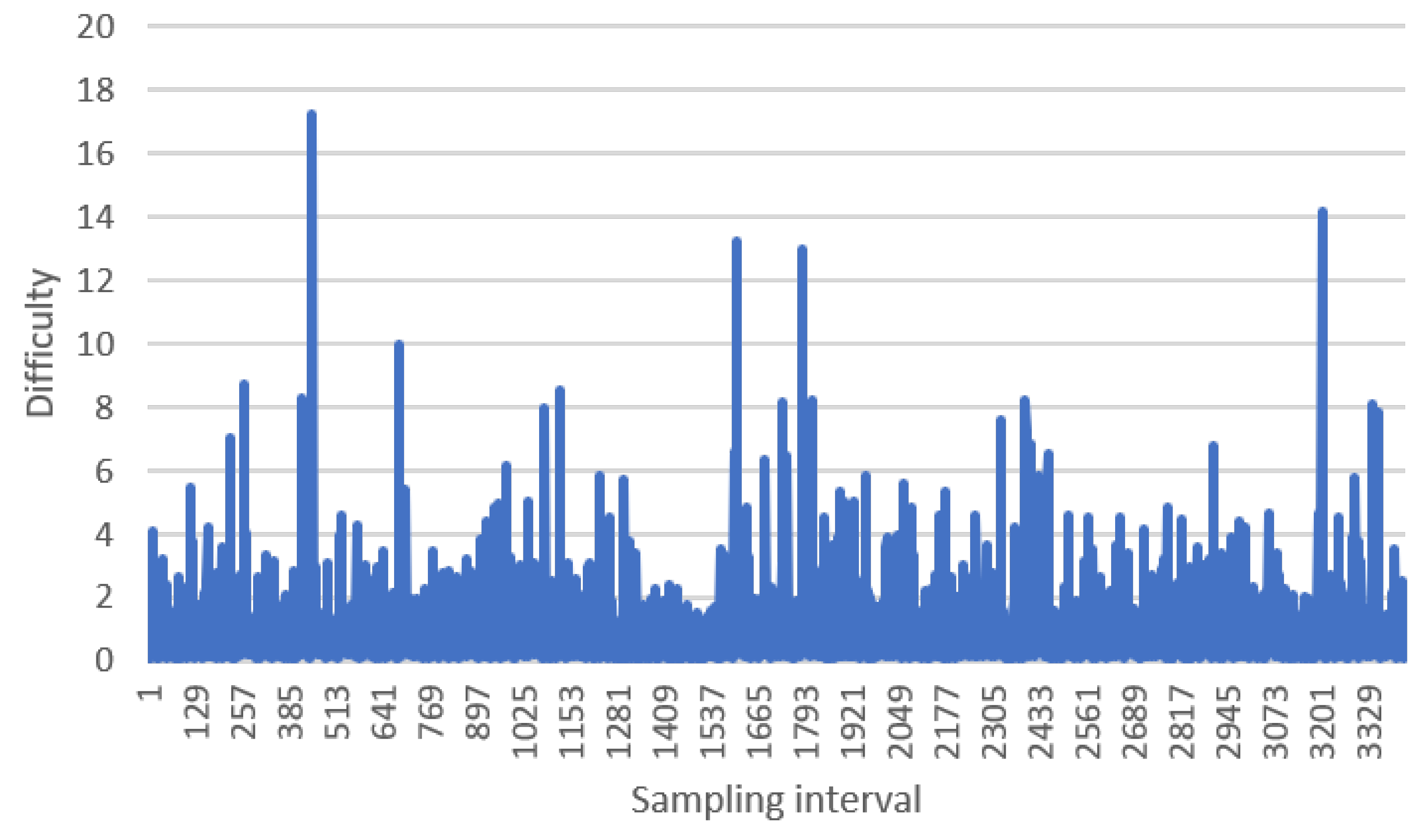
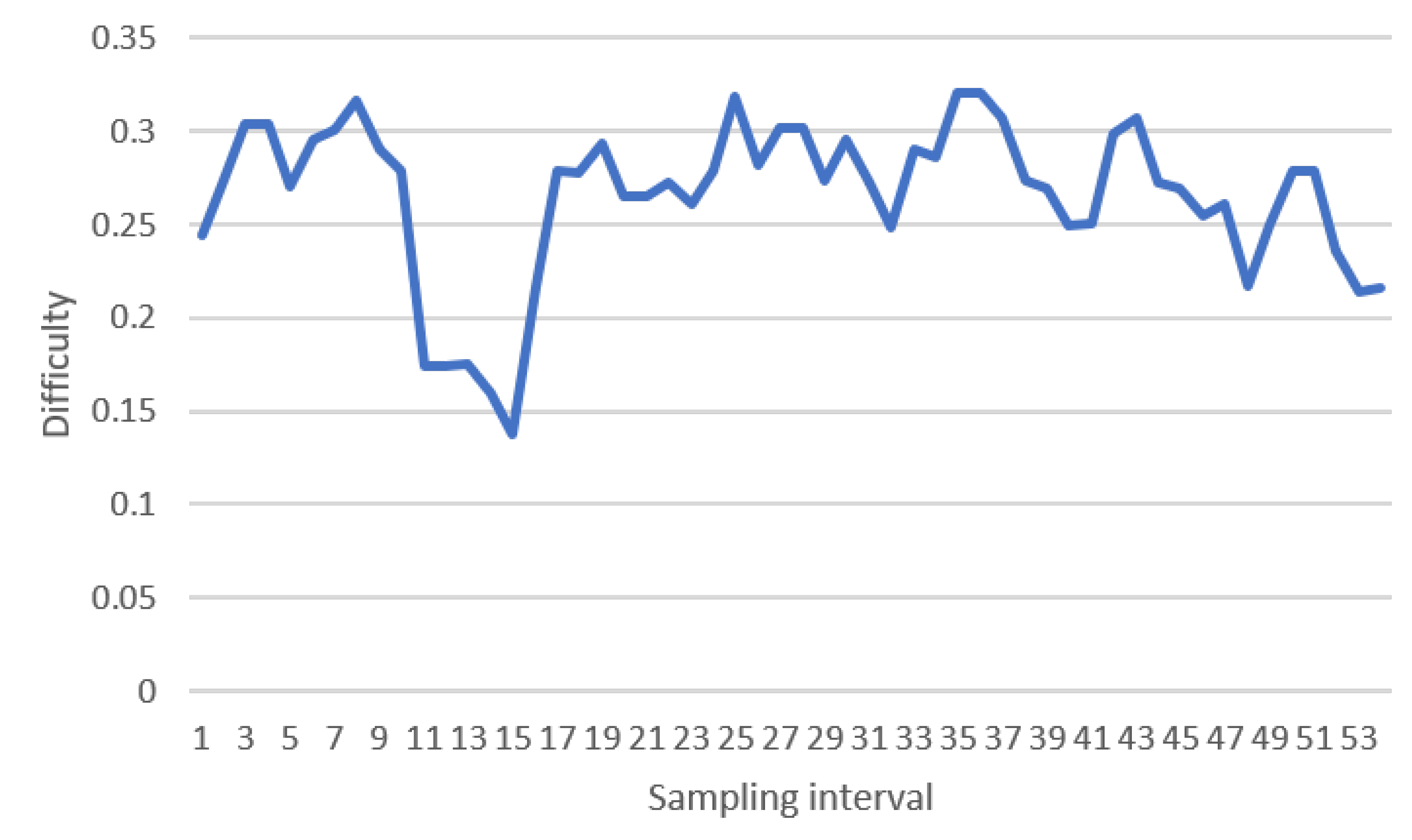
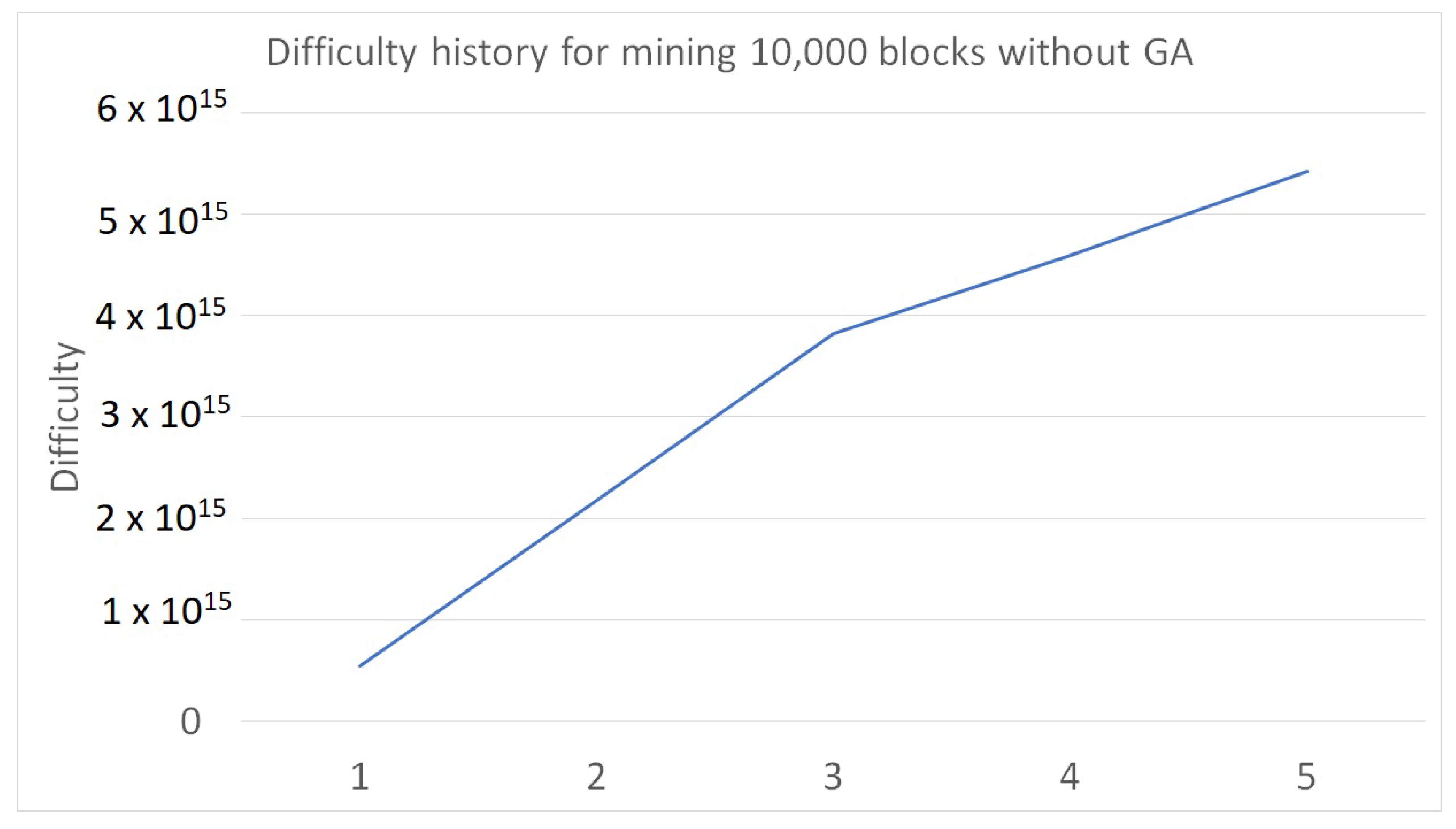
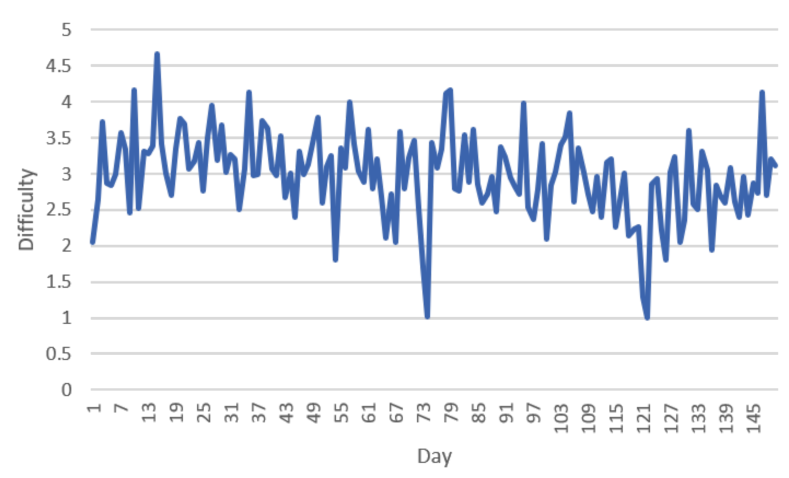
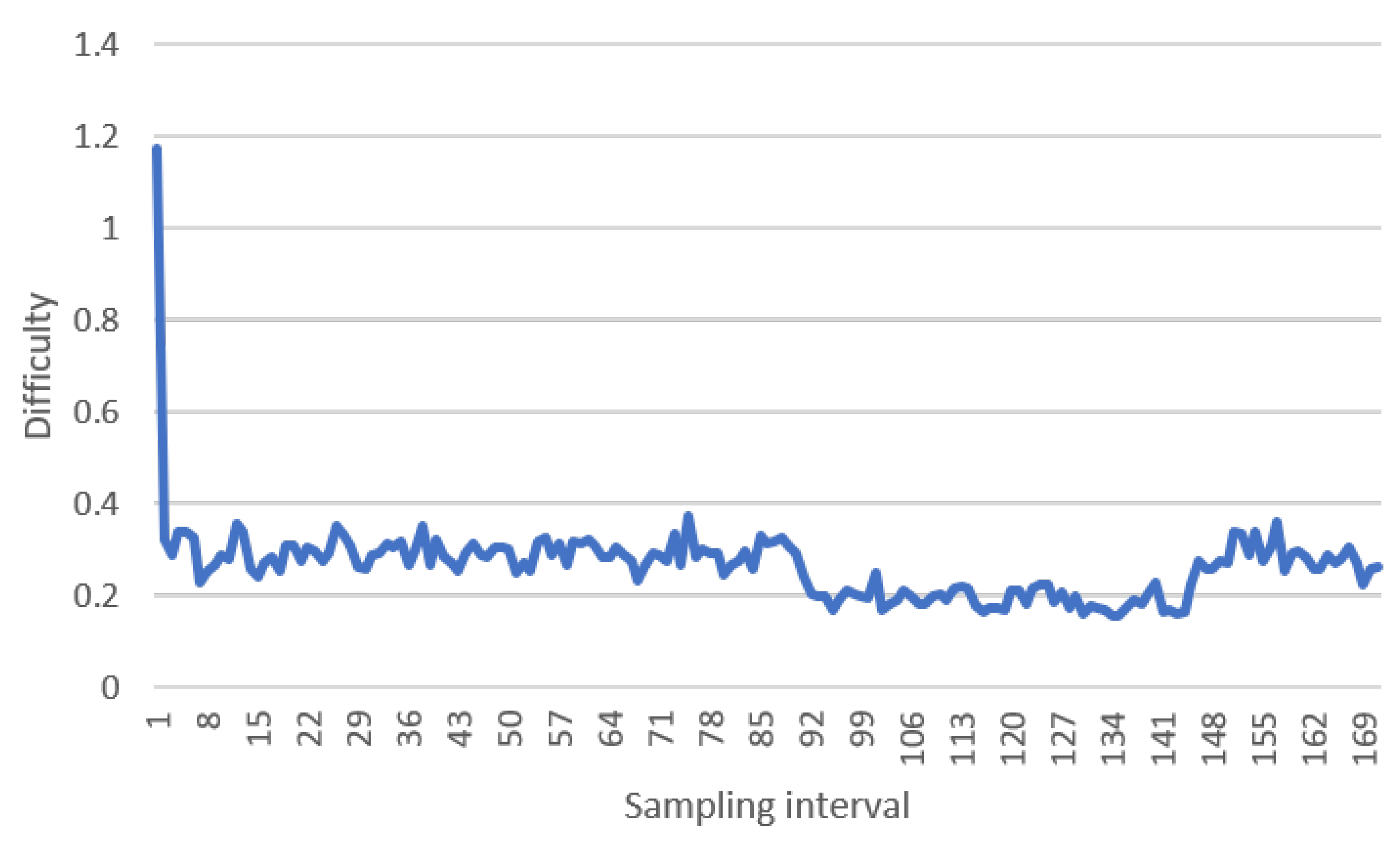
Figure 12 and Figure 13 show the recorded difficulty history for Default and Scenario 4. From Figure 12, without GA, the difficulty was unable to reach the expected value before the mining ended, even after five difficulty adjustments. With GA (Figure 13), the blockchain was quicker to reach the intended difficulty, reaching it just after the third difficulty adjustment, and it was comparatively stable.

4.4. Application Considerations

The average elapsed GA time (population size = 200 and maximum generation = 50) was 165.74 s or 2.7 min during our simulations, with parallel processing enabled, using 10 threads out of a total of 16 threads. A rise in central processing unit (CPU) usage was observed during this period, with a maximum of around 90% with an Intel Xeon E5-2650 v2 processor (2.6 GHz, 8 cores and 16 threads). If the GA was applied on an actual Bitcoin blockchain network, the machines running the nodes may suffer some loss of processing power, and this varies between different hardware specifications. One response is to detect an anomaly or abnormality in the block time. When the average actual block time is greater or smaller than a predetermined threshold, the GA runs in place of the default parameters. Furthermore, to ensure consistency across all the nodes, the total actual time taken to mine the previous N blocks is used as the determinant seed in the GA, otherwise, the nodes may arrive at different parameters and state consensus would be lost.

Although lower standard deviations for average block time and difficulty were obtained, increases in $t_{\mathrm{M}\mathrm{B}\mathrm{P}}$ and $r_s$ were found. Although a stale block is not directly harmful and does not cause major problems on the network, there are a few ways in which it can impact the network slightly, such as causing poor propagation of the network [23]. In addition, double spending is one of the potential problems caused by stale blocks. On 27 January 2020, a USD 3 double-spend from a stale block occurred, which was the first stale block found since 16 October 2019. Because of the low value involved, it was very unlikely to be a targeted attack. In addition, the distributed aspect of a blockchain ensures that the success of an attack depends on managing 51% of the network’s mining hash rate, making these types of attacks nearly impossible. The growing $r_s$ also impacts $t_{\mathrm{M}\mathrm{B}\mathrm{P}}$, as a certain bandwidth is lost when propagating stale blocks, thereby increasing the $t_{\mathrm{M}\mathrm{B}\mathrm{P}}$ whenever $r_s$ is high.

Moreover, the GA was observed to be tending towards a block interval that was as low as possible. This was caused by a low block interval resulting in a low standard deviation of the average block time, which was one of the objective functions. A low block interval such as 1 s gives rise to a high $r_s$, as time is needed to propagate the block. As seen in one study, the longer the network propagation time, the more frequently miners were mining on top of old blocks, hence increasing the stale block rate [24]. It is worth looking at defining a new range for the optimization variables. Block intervals of 1 s or 2 s are not suggested, and therefore these numbers might be removed from the range for better results. In order to increase the GA’s performance, new optimization variables and goal functions may be considered. For example, additional objective functions such as the block propagation time and stale block rate allow the GA to produce better optimization by not focusing solely on low block intervals and difficulty adjustment intervals (to obtain low average block times and difficulties), as they should also decrease the median block propagation time and stale block rate at the same time. However, this could also have an adverse effect, as these objective functions may interfere with the original intention of optimizing the block and difficulty adjustment intervals. On the other hand, decoupling the sliding window from the difficulty adjustment interval for the optimization variables should assist in improving the performance for low difficulty adjustment intervals. Alternatively, the timing of when to activate the GA for optimization and alternative strategies to prevent the GA from continuously optimizing could be examined. This will be the subject of future investigation.

5. Conclusions

A GA was proposed as an optimization approach for the difficulty adjustment intervals of a PoW blockchain. The aim of integrating the GA was to ensure that, by tuning the block and difficulty intervals, the blockchain could respond quickly to any sudden occurrence such as a large decrease or increase in hash rate. Using an evolutionary approach, the GA was expected to evolve to identify suitable intervals for changing the difficulty rates, in order to minimize the standard deviation of the average block time, defined as the time to generate one block. The GA optimized two variables (block interval and difficulty adjustment interval) based on the two objective functions (the standard deviations of average block time and difficulty). The optimal combination of variables was chosen and the new block mined was based on the new parameters.

The suggested difficulty adjustment technique aimed to be reliable enough to reduce the standard deviation of difficulty variations, resulting in minimal volatility. The purpose was to produce equal and consistent difficulty outputs from each chain in the network, while keeping the computation simple. However, issues such as when to activate the GA for optimization and how to prevent the GA from continuously optimizing could also be investigated.