Abstract
Using both analytical and numerical techniques, we discuss wave solutions within the framework of an extended nonlinear Schrödinger equation with constant coefficients equipped with spatiotemporal dispersion, self-steepening effects, and a Raman scattering term. We present the exact traveling wave solution of the system in terms of Jacobi elliptic functions and mention some symmetry results as they relate to the resulting ordinary differential equation. A constructed bright soliton solution serves as the base to compare a numerical solution of the system using spectral Fourier methods with a precise statistical low-rank approximation using a data-driven approach aided by the Koopman operator theory. We found that the spatiotemporal feature added to the model serves as a regularizing tool that enables a precise reconstruction of the original solution.
1. Introduction
The propagation of waves in different media has been the research subject of many scientists in different branches of the natural sciences, engineering, and beyond. Several systems have been proposed to describe the behavior of such waves, and many of them have been based on the pivotal, and 1933 Nobel Prize winning, work of Erwin Schrödinger during 1925–1926 [1]. His landmark study of wave matters later proved to be fundamental for different areas of physics and engineering, and, as a result, various extensions of the original Schrödinger equation have been proposed to study different phenomena (see, for example, [2,3,4,5,6,7]). Analytic results involving extensions of the Schrödinger equation are abundant, with many of them exploring soliton-related solutions. For example, Gomorov and Malomed studied in [4] soliton dynamics considering a nonlinear Schrödinger-type equation (NLSE) from a system describing the interaction between high and low frequency waves. In [5], the same authors explored dynamics of solitons in a different extension of the NLSE to study surface waves. Similarly, Bandelow and Ahkmediev obtained rogue waves solutions [3] of an integrable extension of the NLSE. More recently, Ali et al. considered in [2] another extension of the NLSE exploring solitons and resulting chaotic behaviors. Motivated by recent advances in Koopman theory for partial differential equations and by recent results on wave propagation within hyperbolic metamaterials, we consider a dimensionless model, which is similar to Equation (2) in reference [2], given by the following extended nonlinear Schrödinger equation (eNLSE):
with The first term in the system (1) describes the time evolution of the complex wave function , the parameters a and b describe the second- and third-order dispersion, c captures the spatiotemporal dispersion features, d deals with the cubic nonlinearity (also known as the Kerr law), the parameter e introduces the self-steepening effect, and the last term f describes the Raman scattering effect. It is worth mentioning that symmetries for Schrödinger-type equations have been studied by different researchers [8,9,10,11,12,13,14] highlighting their importance for constructing explicit traveling wave and soliton solutions. Some of the approaches taken on this work are adopted from results available in the literature regarding symmetries of PDEs.
The system (1) is a natural extension of the model derived in [15] by adding spatiotemporal features of a pulse evolving within hyperbolic metamaterials. Thus, we explore wave solutions of the system (1) motivated by recent results in hyperbolic metamaterials. Both numerical and analytical solutions of the systems are presented and compared with the aid of matrix factorization techniques and the theory of data reduction from statistics.
The use of statistical theory to explore the dynamics of nonlinear behavior in deterministic systems, including Schrödinger’s wave equation, has been an essential tool in looking at the same problem but from a completely different point of view. Results during the last few decades have allowed researchers from many institutions to understand and interpret, to a great extent, the mechanisms of nonlinear features embedded within nonlinear systems. Such systems are usually highly dimensional, and few of them can be described analytically. Thus, in many cases, researchers must rely on accessible big data sets, and such a dependency creates many challenges to advancement in the sciences.
Fortunately, different solution methods have been developed to approximate, with high precision, the dynamics governing such complex systems. Transforming a highly multidimensional nonlinear system to a quasilinear reduced one containing the key features of the original one is an example of such an approach and one of our goals for the numerical results section. Different techniques have been proposed to reduce the dimension of model data. Most utilized among these techniques are singular value decomposition (SVD), principal component analysis (PCA), proper orthogonal decomposition (POD), dynamic mode decomposition (DMD), and their corresponding extensions. The idea to decompose and reduce a system into its most relevant structure may have its roots in a pair of papers [16] by B.O. Koopman and [17] by Koopman and J.V. Neumann; in these papers, the authors depicted the possibility of the relation between dynamical properties of a physical system (focusing on classical mechanical systems) with the structure of the corresponding spectrum. During the subsequent decades, many contributions led to the Koopman operator theory, which is basically an operator theoretic approach to analyze dynamical systems. Connected to the underlying nonlinear dynamics through Koopman operator theory is the DMD approach [18,19,20,21,22,23,24].
Although the above reduction methodologies have been focused purely on data, some work has been done also to study the dynamics of nonlinear systems described by equations aiming to handle them in the near future without analytic calculations [24,25,26,27,28,29,30]. The nonlinear Schrödinger equation [25,28,31,32] has been a source for these types of studies for many reasons, one of them been the feasibility of applying it in different areas of research, for example, in quantum computing.
In this work, we construct both a traveling wave solution and a bright soliton solution and compare the latter with its low-rank statistical approximation generated through the Koopman operator approach, which relies on SVD and DMD and generally can be thought of as a data-driven technique to obtain a linear reduced order model for high-dimensional complex systems. The rest of the manuscript is distributed as follows. In Section 2, we construct an analytic expression first for the traveling wave solution and then for a bright soliton solution. In Section 3, we present and compare the numerical approximations resulting from spectral Fourier methods and the Koopman operator based on the soliton solution. Then, we conclude our work with key final remarks.
2. Analytical Results
For the analytical considerations, we first present a traveling wave solution and then a bright soliton solution. The latter will be the starting point for our numerical results.
2.1. Traveling Waves
In this section, we aim to construct the exact traveling wave solution for the eNLSE (1). Assume the system under consideration supports traveling wave solutions of the form
where is the propagation speed of a wave, is the wave number, and is the wave frequency. The parameter is just a phase constant. The substitution of (2) into (1) leads to
for the real part, and
for the imaginary portion. Integrating the last Equation (4) yields
after dividing by b and neglecting the constant of integration. Notice the indisputable resemblance of (5) with the unforced Duffing oscillator. Its symmetries and isotypic components in the space corresponding to the actions of its symmetric group were discussed in [33]. Indeed, one can check also that the system (5) is equivariant (see also [33] for more details).
Since must satisfy both (3) and (5), by equating the corresponding coefficients, one gets the main parameters that describe the waveform, e.g., the wave speed, which is given by
the wave number as
and the frequency takes the form
where Equation (5) is a Painleve type-II equation, and, as stated earlier, its likeness with the unforced–undamped Duffing oscillator nonlinear system is evident; thus, a solution in terms of elliptic functions shall fall out. Following the work of Beléndez et al. in [34], the corresponding solution in terms of Jacobi elliptic functions is given by
where
and
in view of the key parameters (6)–(8) and along with onset conditions and The exact periodic traveling wave solution for the system describing wave propagation in hyperbolic nonlinear materials is given by
where the speed, wave number, and frequency are given by (6), (7), and (8), respectively.
A conventional approach can be applied to the eNLSE system in order to establish traveling waves in terms of hyperbolic functions as well. To construct a traveling wave solution to the system (1) in terms of hyperbolic functions, we first retrieve its corresponding speed from the imaginary part (4), which is given by
whenever the constraints
are satisfied. Notice that (13) differs from the speed of the elliptic solution (6) where the parameter b was preserved. Now, in view of such constraints, Equation (3) reduces into
By multiplying (15) by and integrating once with zero initial conditions, we have
which can be rewritten as
Using integration by parts and a suitable substitution leads to
whose solution can be written in terms of hyperbolic secant if
or in terms of hyperbolic sine if the direction of the last inequality is reversed.
2.2. Bright Soliton
Since we are interested in a soliton solution where as , we assume that the eNLSE (1) supports a solution of the form
where represents the general amplitude, and, in the phase factor, , and describe the frequency of the soliton, the wave number, and a phase constant, respectively. Thus, inserting the solution form (20) into the system (1) and decomposing into real and imaginary parts lead to the speed as in the case for the hyperbolic traveling wave (13),
from the imaginary part provided (14) and the identity
from the real portion. For the case of bright soliton, the still unknown can be written as
where A and B represent the amplitude constant and inverse width correspondingly. The real parameter j will be determined by exploring the balance between nonlinearity and dispersion. One can check that (23) reduces the identity (22) to
where the interplay between nonlinearity and dispersion leads to . The resulting value of j reduces (24) to the following two identities:
and
where the speed was retrieved in (21) as long as
and
are satisfied. Consequently, the bright soliton solution of the system (1) has the form
where the amplitude (25) and the frequency (26) were described in terms of the soliton width, and the speed was described in (21). This solution will exist as long as the conditions given in (14), (27), and (28) are satisfied. The profile of the bright soliton (29) will be essential for the numerical solutions of the system, which we present in the next section.
3. Numerical Approximations
In this section, we discuss the numerical solution of the eNLSE (1) using two different approaches. First, we construct a numerical solution (the data) using standard spectral Fourier methods. Then, we apply the dynamic mode decomposition algorithm and Koopman operator approaches to build a statistical low-rank approximation of the wave dynamics embedded in the system with the least possible data.
3.1. Spectral Fourier Methods
While many numerical methods to solve partial differential equations exist, most prominent during the last decades are finite difference methods, finite element methods, gradient discretization methods, and spectral methods. The first three methods are based on local representation of functions while the last makes use of global representation and, thus, usually yields higher order accuracy. The spectral approximation methods to solve PDEs are both efficient and highly accurate and, in our case, based on the Fourier transform to accommodate the highly periodic behavior of the wave dynamics embedded within the examined system. We denote the Fourier transform (FT) of by:
For simplicity, we use instead of One can notice that the transform leads to a result in terms of the wave number k from the original state space x, and such a result is a vector of Fourier coefficients. A straightforward calculation of the FT of the eNLSE (1) yields
for each k. Thus, the FT provides a representation of the time series dynamics in the Fourier space, allowing us to solve the transformation with known iterative schemes or available built-in functions in the computing environment of preference.
A finite but sufficiently representative space domain, e.g., is selected so that, at the boundaries, the function is well approximated by zero. This resembles the fact that as The time domain is while the frequency domain will be properly constructed. The initial condition to be considered is in view of the bright soliton amplitude (23). In Figure 1, the time evolution of the solution profile using spectral methods is provided for to depict a better view, in terms of its intensity, and in terms of its corresponding contour. As expected, the wave approximation reveals the periodic behavior typical of many Schrödinger-type equations. We will consider this solution as our original data and will compare with its statistical low-rank counterpart approximation on the next subsections.
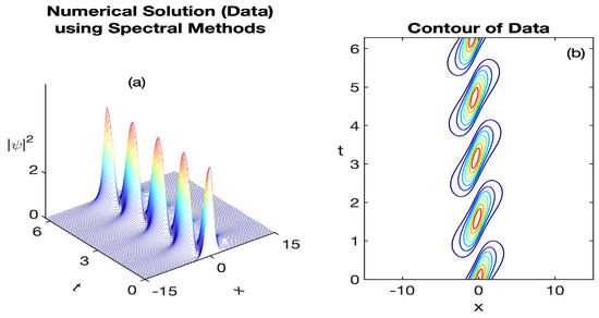
Figure 1.
Representation of the numerical approximation using spectral Fourier methods depicting oscillatory wave propagation: (a) the time evolution of the oscillatory wave profile (the constructed data) and (b) the corresponding contour plot.This simulation considers the parameter values a = 2.09754, b = −0.0121, c = 16.8998, d = 0.0789, e = 3.7437, f = 0.0398, and time frame .
3.2. Dynamic Mode Decomposition
Arising from the fluid dynamics community, the Dynamic Mode Decomposition (DMD) is a purely data-driven technique aimed to extract spatio-temporal, coherent structures, or patterns that dominate the observed measurement data, from the system under consideration. The key ingredient of the DMD recipe is the Singular Value Decomposition (SVD), a numerically stable matrix factorization technique used to obtain an optimal low-rank approximation of highly dimensional systems and to calculate pseudo-inverses of non-square arrays that allows for determining the least squares and minimum solutions of a linear matrix system of the form . Thus, for every complex-valued matrix , its exact SVD approximation is where both and are unitary matrices, while is a matrix containing the singular values of such that those values are ordered from the largest to the smallest [35,36]. Here, represents the conjugate transpose of matrix V, and denotes the More–Penrose pseudoinverse of matrix The aim of this process is to retrieve the eigen-decomposition of matrix , which contains the dominant coherent patterns of the system under study, without having to compute A. In several situations, the smallest singular value is zero (e.g., when X is not full row-rank); thus, the rank of the matrix may serve as a point of reference to truncate the SVD while still preserving the key features of the dominant patterns. For a truncation value the truncated SVD to approximate X is now where the value of r is selected according to the situation at hand. The amount of toleration in the selection of r is usually tied to the specifics of the given nonlinear system. Therefore, the role of the SVD in the DMD scheme will be to facilitate a lower rank approximation of the original system while keeping its dominant patterns.
Having established the idea behind the SVD method, we proceed to discuss the DMD scheme following the reasoning of Kutz et al. [35], which first requires a data set of the form:
where usually it is expected the number of rows to be considerably larger than the number of columns. In this work, we arrange the columns into the desired matrix X as presented above in (31). Once we have constructed our data matrix, the DMD algorithm can be implemented as follows:
- Create two matrices from data set given in (31):
- Compute the full rank SVD of
- Based on the selected rank , construct the reduced matrices , , and
- Construct the dynamic operator
- Compute eigenvalues and eigenvectors of
- Construct the modes (eigenvectors) of the original matrix
- Construct time series approximation of the original dynamical system:where are the eigenvalues of L and are the initial conditions.
The DMD scheme will be an essential tool to construct the Koopman approximation of the wave dynamics embedded in the eNLSE (1) in the following subsection.
3.3. Koopman Approximation
Another approach for analyzing nonlinear systems is based on the Koopman operator which relies on the DMD algorithm for its corresponding computations. This approach has recently been adopted by several research groups by including Kernel observables [37,38,39,40,41,42,43,44,45]. The initial success of the DMD in fluid mechanics has led to a large number of similar algorithms being proposed for the computation of the Koopman spectral properties, which seek to approximate with a best fit linear model [27,29]. Arbabi and Mezić proved that applying DMD to data arranged in a Hankel-type matrix produces the true Koopman eigenfunctions and eigenvalues [27]. Kutz showed that an observable based on the nonlinearity present in the NLSE gives an approximation whose error is orders of magnitude smaller than the standard DMD. Indeed, for certain systems, the right choice of observable function can linearize the nonlinear manifold on which the system evolves. Typically, analytical expressions for such systems are unavailable, and, as a result, a data-driven approach could be advantageous.
The Koopman operator aims to linearize the manifold in which the nonlinear state dynamics are embedded by projecting into a lower dimensional, weakly nonlinear subspace. Consider a continuous-time dynamical system where x is the state on a smooth n-dimensional manifold M and f is a nonlinear vector-valued function of the same dimension as x. The Koopman operator acts on the space of all scalar observable functions such that
The typical approach to analyzing nonlinear systems is to linearize the dynamics (which we may not know) in the neighborhood of the critical points, however, the Koopman operator attempts to linearize the state space M itself, providing a global linear representation of the dynamics that is valid far from fixed points and periodic orbits [29]. The operator acts on a complete linear vector space, so admits an eigen-expansion which completely characterizes the dynamics of the system [26]. The eigenpairs of are used to construct the Koopman modes, which are of particular interest since projection of the observable functions allow the system dynamics to be advanced essentially by scalar multiplication. In the case of the system (1), the chosen observables are strictly based on the cubic nonlinear term.
The accuracy of the Koopman reconstruction relies mostly on the selection of the observable function. The Figure 2 depicts the reconstructed dynamics of the eNLSE using Koopman theory after considering for the observable function only the cubic nonlinear part In our work, the spatio-temporal term play a key role in obtaining the desired approximation. By comparing (a) in Figure 1 and Figure 2, one can appreciate the precise approximation of the Koopman results with the wave dynamics of the eNLSE. The spectra in Figure 2c is approximately purely imaginary, as desired, highlighting the higher precision of the reconstruction. Truncating at , and using the observable base on the cubic nonlinearity lead to a good approximation of the dynamics of the eNLSE.
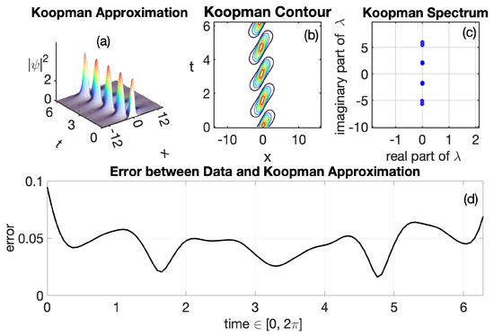
Figure 2.
Numerical results using Koopman Decomposition. (a) Koopman wave approximation profile reconstructing the data provided on Figure 1a. (b) Contour of the corresponding Koopman profile depicting the same dynamics as in Figure 1b. (c) Spectrum of the Koopman operator for a rank of . The nearly pure imaginary spectrum reflects the high quality of the reconstruction. (d) Error measured in the least-square sense between the resulting profile from Spectral Methods and the profile yielded by Koopman Theory of the given system. The parameter values considered are with The case when yields nearly the same results as well as when with .
4. Conclusions
The understanding of wave propagation in Schrödinger-type systems is still important due to the possible wide range of applications, from communication systems to the emerging field of quantum computing. The study of the dynamics embedded in a nonlinear system using the methods discussed on this work has been of great interest during the last years due to its possible positive impact in the understanding of the hidden dynamics in data sets. The idea of using only a portion of the data to construct a precise generalization is definitely, in terms of numerical calculations, a cost-effective process. Dimension reduction techniques to approximate the desired outputs in the most possible precise way are desired essential elements in data science. In this work, we explored analytical and numerical wave solutions of a highly nonlinear extension of the original Schrödinger equation motivated by recent results in the field of material sciences. We found that the spatio-temporal dispersion term served as a key regularization tool on the numerical algorithm for the Koopman reconstruction of the profile created with Spectral Methods on Figure 1. The almost purely imaginary resulting Koopman spectrum corroborates the precision of the reconstruction. The dynamic decomposition algorithm is a landmark in the study of the hidden dynamics embedded in data, and recent progress indicates it works. However, much work is still needed to determine a process to construct the exact observables for each case in the Koopman approach. We hope that the results presented in this work will contribute to the advancement of understanding the dynamics within systems described by data. The ability of the spatio-temporal dispersion in balancing the dynamics of highly nonlinear Schrödinger-type equations is essential to reach the desired accuracy approximation of embedded dynamics [46]. Further work on this subject is still necessary to develop a framework to decide a precise observable function to better understand the influence the spatio-temporal term and to identify possible corresponding advantages.
Author Contributions
Conceptualization, methodology, formal analysis, and investigation, R.K., A.P. and J.M.V.-G.; writing original draft preparation, review and editing, R.K., A.P. and J.M.V.-G.; supervision and project administration, J.M.V.-G. All authors have read and agreed to the published version of the manuscript.
Funding
NSF-DMS Award Number # 1757717.
Institutional Review Board Statement
Not applicable.
Informed Consent Statement
Not applicable.
Data Availability Statement
Not applicable.
Acknowledgments
The authors acknowledge the effort, guidance, comments, advise and patience from all faculty members involved in the REU@LU 2021. This study was supported by the National Sciences Foundation (NSF Award # 1757717).
Conflicts of Interest
The authors declare no conflict of interest.
References
- Schrödinger, E. Quantisierung als Eigenwertproblem (Erste Mitteilung). Ann. Phys. 1926, 79, 361–376. [Google Scholar] [CrossRef]
- Ali, F.; Jhangeer, A.; Muddasser, M.; Almusawa, H. Solitonic, quasi-periodic, super nonlinear and chaotic behaviors of a dispersive extended nonlinear Schrödinger equation in an optical fiber. Results Phys. 2021, 31, 104921. [Google Scholar] [CrossRef]
- Bandelow, U.; Akhmediev, N. Persistence of rogue waves in extended nonlinear Schrödinger equations: Integrable Sasa-Satsuma case. Phys. Lett. 2012, 376, 1558–1561. [Google Scholar] [CrossRef]
- Gromov, E.M.; Malomed, B.A. Damped solitons in an extended nonlinear Schrödinger equation with a spatial stimulated Raman scattering and decreasing dispersion. Opt. Commun. 2014, 320, 88–93. [Google Scholar] [CrossRef][Green Version]
- Gromov, E.M.; Malomed, B.A. Solitons in a forced nonlinear Schrödinger equation with the pseudo-Raman effect. Phys. Rev. E 2015, 92, 062926. [Google Scholar] [CrossRef]
- Vega-Guzmán, J.M.; Biswas, A.; Mahmood, M.F.; Zhou, Q.; Moshokoa, S.P.; Belic, M. Optical solitons with polarization mode dispersion for Lakshmanan-Porsezian-Daniel model by the method of undetermined coefficients. Optik 2018, 171, 114–119. [Google Scholar] [CrossRef]
- Zhang, Z.; Liu, Z.; Miao, X.; Chen, Y. Qualitative analysis and traveling wave solutions for the perturbed nonlinear Schrödinger’s equation with Kerr law nonlinearity. Phys. Lett. A 2011, 375, 1275–1280. [Google Scholar] [CrossRef]
- Gagnon, L.; Winternitz, P. Lie symmetries of a generalized nonlinear Schrödinger equation: I. The symmetry group and its subgroups. J. Phys. Math. Gen. 1988, 21, 1493. [Google Scholar] [CrossRef]
- Panoiu, N.C.; Mihalache, D.; Mazilu, D.; Crasovan, L.C.; Mel’nikov, I.V.; Lederer, F. Soliton dynamics of symmetry-endowed two-soliton solutions of the nonlinear Schrödinger equation. Chaos 2000, 10, 625–640. [Google Scholar] [CrossRef]
- Popovych, R.O.; Kunzinger, M.; Eshraghi, H. Admissible transformations and normalized classes of nonlinear Schrödinger equations. Acta Appl. Math. 2010, 109, 315–359. [Google Scholar] [CrossRef]
- Peng, L. Symmetries and reductions of integrable nonlocal partial differential equations. Symmetry 2019, 11, 884. [Google Scholar] [CrossRef]
- Biswas, A.; Vega-Guzman, J.; Bansal, A.; Kara, A.H.; Alzahrani, A.K.; Zhou, Q.; Belic, M.R. Optical dromions, domain walls and conservation laws with Kundu-Mukherjee-Naskar equation via traveling waves and Lie symmetry. Results Phys. 2020, 16, 102850. [Google Scholar] [CrossRef]
- Huang, Y.; Jing, H.; Li, M.; Ye, Z.; Yao, Y. On Solutions of an Extended Nonlocal Nonlinear Schrödinger Equation in Plasmas. Mathematics 2020, 8, 1099. [Google Scholar] [CrossRef]
- Myrzakul, A.; Nugmanova, G.; Serikbayev, N.; Myrzakulov, R. Surfaces and Curves Induced by Nonlinear Schrödinger-Type Equations and Their Spin Systems. Symmetry 2021, 13, 1827. [Google Scholar] [CrossRef]
- Boardman, A.D.; Alberucci, A.; Assanto, G.; Grimalsky, V.V.; Kibler, B.; McNiff, J.; Nefedov, I.S.; Rapoport, Y.G.; Valagiannopoulos, C.A. Waves in hyperbolic and double negative metamaterials including rogues and solitons. Nanotechnology 2017, 28, 444001. [Google Scholar] [CrossRef] [PubMed][Green Version]
- Koopman, B.O. Hamiltonian systems and transformation in Hilbert space. Proc. Natl. Acad. Sci. USA 1931, 17, 315–318. [Google Scholar] [CrossRef] [PubMed]
- Koopman, B.O.; Neumann, J.v. Dynamical systems of continuous spectra. Proc. Natl. Acad. Sci. USA 1932, 18, 255–263. [Google Scholar] [CrossRef] [PubMed]
- Mezić, I.; Banaszuk, A. Comparison of systems with complex behavior. Phys. D Nonlinear Phenom. 2004, 197, 101–133. [Google Scholar] [CrossRef]
- Mezić, I. Spectral properties of dynamical systems, model reduction and decompositions. Nonlinear Dyn. 2005, 41, 309–325. [Google Scholar] [CrossRef]
- Rowley, S.W.; Mezić, I.; Bagheri, S.; Schlatter, P.; Henningson, D.S. Spectral analysis of nonlinear flows. J. Fluid Mech. 2009, 641, 115–127. [Google Scholar] [CrossRef]
- Schmid, P.J.; Li, L.; Pust, O. Applications of the dynamic mode decomposition. Theor. Comput. Fluid Dyn. 2011, 25, 249–259. [Google Scholar] [CrossRef]
- Noack, B.R.; Afanasiev, K.; Morzynski, M.; Tadmor, G.; Thiele, F. A hierarchy of low-dimensional models for the transient and post-transient cylinder wake. J. Fluid Mech. 2003, 497, 335–363. [Google Scholar] [CrossRef]
- Tu, J.H.; Rowley, C.W.; Luchtenburg, D.M.; Bruntin, S.L.; Kutz, J.N. On dynamic mode decomposition: Theory and applications. J. Comput. Dyn. 2014, 1, 391–421. [Google Scholar] [CrossRef]
- Alla, A.; Kutz, J.N. Nonlinear model order reduction via dynamic mode decomposition. Siam J. Sci. Comput. 2017, 39, B778–B796. [Google Scholar] [CrossRef]
- Crabb, M.; Akmediev, N. Doubly periodic solutions of the class-I infinitely extended nonlinear Schrödinger equation. Phys. Rev. E 2019, 99, 052217. [Google Scholar] [CrossRef]
- Kutz, J.N.; Proctor, J.L.; Brunton, S.L. Koopman theory for partial differential equations. arXiv 2016, arXiv:1607.07076. [Google Scholar]
- Arbabi, H.; Mezic, I. Ergodic Theory, Dynamic Mode Decomposition and Computation of Spectral Properties of the Koopman Operator. arXiv 2017, arXiv:1611.06664v6. [Google Scholar] [CrossRef]
- Kutz, J.N.; Proctor, J.L.; Brunton, S.L. Applied Koopman Theory for Partial Differential Equations and Data-Driven Modeling of Spatio-Temporal Systems. Complexity 2018, 2018, 16. [Google Scholar]
- Brunton, S.L.; Brunton, B.W.; Proctor, J.L.; Kaiser, E.; Kutz, J.N. Chaos as an intermittently forced linear system. Nat. Commun. 2017, 8, 1–9. [Google Scholar] [CrossRef]
- Nakao, H.; Mezić, I. Spectral analysis of the Koopman operator for partial differential equations. Chao Interdiscip. J. Nonlinear Sci. 2020, 30, 113131. [Google Scholar] [CrossRef]
- Ekici, M.; Mirzazadeh, M.; Sonmezoglu, A.; Ullah, M.Z.; Asma, M.; Zhou, Q.; Moshokoa, S.P.; Biswas, A.; Belic, M. Optical solitons with Schrödinger–Hirota equation by extended trial equation method. Optik 2017, 135, 451–461. [Google Scholar] [CrossRef]
- Islam, W.; Younis, M.; Rizvi, S.T.R. Optical Solitons with time fractional nonlinear Schrödinger equation and competing weakly nonlocal nonlinearity. Optik 2017, 130, 562–567. [Google Scholar] [CrossRef]
- Salova, A.; Emenheiser, J.; Rupe, A.; Crutchfield, J.P.; D’Souza, R.M. Koopman operator and its approximations for systems with symmetries. Chaos Interdiscip. J. Nonlinear Sci. 2019, 29, 093128. [Google Scholar] [CrossRef]
- Beléndez, A.; Beléndez, T.; Matínez, F.J.; Pascual, C.; Alvarez, M.L.; Arribas, E. Exact solution for the unforced Duffing oscillator with cubic and quintic nonlinearities. Nonlinear Dyn. 2016, 86, 1687–1700. [Google Scholar] [CrossRef]
- Kutz, J.N.; Brunton, S.L.; Brunton, B.W.; Proctor, J.L. Dynamic Mode Decomposition: Data-Driven Modeling of Complex Systems; Society for Industrial and Applied Mathematics (SIAM): Philadelphia, PA, USA, 2018. [Google Scholar]
- Gao, Z.; Lin, Y.; Sun, X.; Zeng, X. A reduced order method for nonlinear parameterized partial differential equations using dynamic mode decomposition coupled with k-nearest-neighbors regression. J. Comput. Phys. 2021, 452, 110907. [Google Scholar] [CrossRef]
- Kawahara, Y. Dynamic mode decomposition with reproducing kernels for Koopman spectral analysis. Adv. Neural Inf. Process. Syst. 2016, 29, 911–919. [Google Scholar]
- Tang, H.Z. Koopman Reduced Order Control for Three Body Problem. Mod. Mech. Eng. 2019, 9, 20–29. [Google Scholar] [CrossRef]
- Kevrekidis, I.; Rowley, C.W.; Williams, M. A kernel-based method for data-driven Koopman spectral analysis. J. Comput. Dyn. 2016, 2, 247–265. [Google Scholar]
- Kaiser, E.; Kutz, J.N.; Brunton, S.L. Data-driven discovery of Koopman eigenfunctions for control. Mach. Learn. Sci. Technol. 2021, 2, 035023. [Google Scholar] [CrossRef]
- Mendible, A.; Koch, J.; Lange, H.; Brunton, S.L.; Kutz, J.N. Data-driven modeling of rotating detonation waves. Phys. Rev. Fluids 2021, 6, 050507. [Google Scholar] [CrossRef]
- Klus, S.; Nüske, F.; Peitz, S.; Niemann, J.H.; Clementi, C.; Schütte, C. Data-driven approximation of the Koopman generator: Model reduction, system identification, and control. Physica D Nonlinear Phenom. 2020, 406, 132416. [Google Scholar] [CrossRef]
- Klus, S.; Nske, F.; Hamzi, B. Kernel-based approximation of the Koopman generator and Schrödinger operator. Entropy 2020, 22, 722. [Google Scholar] [CrossRef] [PubMed]
- Balabane, M.; Méndez, M.A.; Najem, S. Koopman operator for Burgers’s equation. Phys. Rev. Fluids 2021, 6, 064401. [Google Scholar] [CrossRef]
- Mesbahi, A.; Bu, J.; Mesbahi, M. Nonlinear observability via Koopman analysis: Characterizing the role of symmetry. Automatica 2021, 124, 109353. [Google Scholar] [CrossRef]
- Phillips, A. Extending Nonlinear Schrödinger Equation to Include Spatiotemporal Dispersion. Master’s Thesis, Lamar University, Beaumont, TX, USA, May 2020. [Google Scholar]
Publisher’s Note: MDPI stays neutral with regard to jurisdictional claims in published maps and institutional affiliations. |
© 2022 by the authors. Licensee MDPI, Basel, Switzerland. This article is an open access article distributed under the terms and conditions of the Creative Commons Attribution (CC BY) license (https://creativecommons.org/licenses/by/4.0/).