Coupled Fractional Traveling Wave Solutions of the Extended Boussinesq–Whitham–Broer–Kaup-Type Equations with Variable Coefficients and Fractional Order

Abstract

In this paper, we propose the extended Boussinesq–Whitham–Broer–Kaup (BWBK)-type equations with variable coefficients and fractional order. We consider the fractional BWBK equations, the fractional Whitham–Broer–Kaup (WBK) equations and the fractional Boussinesq equations with variable coefficients by setting proper smooth functions that are derived from the proposed equation. We obtain uniformly coupled fractional traveling wave solutions of the considered equations by employing the improved system method, and subsequently their asymmetric behaviors are visualized graphically. The result shows that the improved system method is effective and powerful to find explicit traveling wave solutions of the fractional nonlinear evolution equations.

1. Introduction

Nonlinear partial differential equations (NPDEs) play an important role to describe nonlinear physical phenomena that can be described by the solutions of NPDEs rising in physics, biology, chemistry, mechanics and mathematical engineering. Moreover, the fractional NPDEs may model physical phenomena better than the general NPDEs. Recently, many powerful techniques have been proposed to obtain explicit wave solutions of nonlinear evolution equations as follows: Khan and Akbar used an enhanced $(G^{\prime }/G)$-expansion method to find explicit solutions of the Variant Boussinesq equations [1,2,3,4,5] by the variational principle; Tian and Qiu a used direct method to obtain explicit solutions of WBK equations, which describe the propagation of shallow water waves, with different dispersion relations [6]; Z. Zhang et al. obtained exact solutions and symmetry reductions for calculating symmetry and exact solutions [7]; Mohyud-Din et al. discussed traveling wave solutions of WBK equations by a homotopy perturbation method [8]; a hyperbolic function method was applied to find solitary wave solution for WBK equations [9]; the Adomian Decomposition Method was used to find exact and numerical solutions of WBK equations [10], and so on. As a result, explicit wave solutions of the fractional nonlinear evolution equations have great significance to reveal internal mechanisms of physical phenomena as fractional orders. Moreover, the closed-form solutions of the fractional nonlinear evolution equations could assist numerical researchers to evaluate the correctness of their results by comparison and help them in stability analysis.

X. F. Yang et al. suggested the variant BWBK-type equations as follows;

$$\begin{array}{c}\hfill \left\{\begin{array}{c}{v}_t+{\left(vf\left(u\right)\right)}_x+{\left(g\left(u_x\right)\right)}_{xx}+{\left(h\left(u\right)\right)}_x-\beta v_{xx}=0,\hfill \\ u_t+{\left(r\left(v\right)\right)}_x+{\left(\int f\left(u\right)du\right)}_x+\beta u_{xx}=0,\hfill \end{array}\right.\end{array}$$

(1)

where $f,g,h,r$ are smooth functions, and $\beta$ is a constant [11].

The present paper is based on Equation (1), and we propose the extended BWBK-type equations with variable coefficients and fractional order as follows:

$$\begin{array}{c}\hfill \left\{\begin{array}{c}\frac{{\partial }^{\alpha }V}{\partial t^{\alpha }}+\frac{{\partial }^{\alpha }}{\partial x^{\alpha }}\left[Vf\left(U\right)\right]+a\left(t\right)\frac{{\partial }^{2\alpha }}{\partial x^{2\alpha }}\left[g\left(\frac{{\partial }^{\alpha }U}{\partial x^{\alpha }}\right)\right]-b\left(t\right)\frac{{\partial }^{2\alpha }V}{\partial x^{2\alpha }}=0,\hfill \\ \frac{{\partial }^{\alpha }U}{\partial t^{\alpha }}+\frac{{\partial }^{\alpha }}{\partial x^{\alpha }}\left[r\left(V\right)+\int f\left(U\right)dU\right]+\frac{{\partial }^{2\alpha }}{\partial x^{2\alpha }}\left[b\left(t\right)(U-h\left(U\right))+c\left(t\right)\frac{{\partial }^{\alpha }U}{\partial t^{\alpha }}\right]=0,\hfill \end{array}\right.\end{array}$$

(2)

where $f\left(U\right),g\left({\partial }^{\alpha }U/\partial x^{\alpha }\right) \mathrm{and} r\left(V\right)$ are smooth functions, and $a\left(t\right),b\left(t\right) \mathrm{and} c\left(t\right)$ are integrable functions on t.

The remainder of this paper is organized as follows: in Section 2, we define the conformable fractional derivative and describe the improved system for obtaining explicit traveling wave solutions of NPDEs in detail. In Section 3, we present the coupled fractional traveling wave solutions of the fractional BWBK equations, the fractional WBK equations and the fractional Boussinesq equations with variable coefficients by using a mathematical computation method and show several dynamical behaviors of the coupled fractional traveling wave solutions that contain exponential-type wave solutions based on suitable values of physical parameters. Some conclusions are given in the end.

2. Prelimiraries

In this section, we introduce the conformable fractional derivative to convert the fractional NPDEs into the nonlinear ordinary differential equations (ODEs) [12,13]. We also introduce the steps of finding the fractional traveling wave solutions of the fractional NPDEs by the improved system method.

2.1. The Basic Definition

Now we define the conformable fractional derivative as follows [14,15]:

Definition 1.

Given a function $f:(0,+\infty )\to \mathbb{R}$, then the conformable fractional derivative of a function f is defined by

$$\begin{array}{c}\hfill {}_t{D}^{\alpha }f\left(t\right)=\underset{ϵ\to 0}{lim}\frac{f(t+ϵt^{1-\alpha })-f\left(t\right)}{ϵ},\end{array}$$

where $t>0$ and $\alpha \in (0,1]$.

The conformable fractional derivatives for some familiar functions give important rules as follows:

$$\begin{array}{c}\hfill {}_t{D}^{\alpha }{t}^r=r{t}^{r-\alpha },r\in \mathbb{R},\\ \hfill {}_t{D}^{\alpha }\left(f\left(t\right)g\left(t\right)\right)=f\left(t\right){}_t{D}^{\alpha }g\left(t\right)+g\left(t\right){}_t{D}^{\alpha }f\left(t\right),\\ \hfill {}_t{D}^{\alpha }\left((f\circ g)\left(t\right)\right)=t^{1-\alpha }{g}^{\prime }\left(t\right)f^{\prime }\left(g\left(t\right)\right),\\ \hfill {}_t{D}^{\alpha }\left(\frac{f\left(t\right)}{g\left(t\right)}\right)=\frac{g\left(t\right){}_t{D}^{\alpha }f\left(t\right)-f\left(t\right){}_t{D}^{\alpha }g\left(t\right)}{g^2\left(t\right)}.\end{array}$$

2.2. The Improved System Method with Parameter Functions

We provide a short description of the improved system method with parameter functions for constructing the explicit solutions of the fractional NPDEs. Consider the fractional NPDEs with respect to independent variables $t,x$ by

$$\begin{array}{c}\hfill {\mathcal{P}}^{}(U,D_t^{\alpha }U,D_x^{\alpha }U,D_t^{2\alpha }U,D_x^{2\alpha }U,\cdots )=0,\end{array}$$

(3)

where $D_t^{\alpha }U,D_x^{\alpha }U,D_t^{2\alpha }U,D_x^{2\alpha }U,\dots$, are the fractional partial derivatives of $U=U(t,x)$ as defined above. Furthermore, $\mathcal{P}$ represents a polynomial in U and its various fractional partial derivatives, which the linear derivative terms and the nonlinear terms are involved. Let us consider the following steps to obtain the fractional traveling wave solutions of Equation (3).

Step 1.

Substituting the unknown functions are $U(x,t)=\mathsf{u}\left(\zeta \right)$ by using the fractional traveling wave variable as

$$\begin{array}{c}\hfill \zeta =k\frac{x^{\alpha }}{\alpha }-{\int }_0^T\omega \left(\tau \right)d\tau ,T=\frac{t^{\alpha }}{\alpha },\end{array}$$

(4)

where k is an arbitrary constant and $\alpha \in (0,1]$, we have the nonlinear ODEs for $\mathsf{u}=\mathsf{u}\left(\zeta \right)$ as follows:

$$\begin{array}{c}\hfill \mathcal{Q}(\mathsf{u},{\mathsf{u}}^{\prime },{\mathsf{u}}^{″},{\mathsf{u}}^{‴},\dots )=0,\end{array}$$

(5)

where ${\mathsf{u}}^{\prime }=d\mathsf{u}/d\zeta ,{\mathsf{u}}^{″}=d^2\mathsf{u}/d{\zeta }^2,{\mathsf{u}}^{‴}=d^3\mathsf{u}/d{\zeta }^3,$ and so on.

Step 2.

Consider the improved system with time-dependent parameters as follows [16,17,18,19,20]:

$$\begin{array}{c}\hfill \left\{\begin{array}{c}{\psi }^{\prime }\left(\zeta \right)=p\left(t\right)\psi \left(\zeta \right),\hfill \\ {\varphi }^{\prime }\left(\zeta \right)=p\left(t\right)\psi \left(\zeta \right)+q\left(t\right)\varphi \left(\zeta \right),\hfill \end{array}\right.\end{array}$$

(6)

where $p\left(t\right)$, $q\left(t\right)$ are integrable parameters depending on t. Equation (6) permits the ans$\ddot{\mathrm{a}}$tz [21]

$$\begin{array}{c}\hfill \left[\frac{\psi \left(\zeta \right)}{\varphi \left(\zeta \right)}\right]=\frac{p\left(t\right)-q\left(t\right)}{p\left(t\right)-q\left(t\right)exp\{-(p\left(t\right)-q\left(t\right)\left)\zeta \right\}},\end{array}$$

(7)

where $p\left(t\right)$, $q\left(t\right)$ are nonzero integrable functions with $p\left(t\right)\ne q\left(t\right)$. On the other hand, when $p\left(t\right)=q\left(t\right)$, we have the ans$\ddot{\mathrm{a}}$tz

$$\begin{array}{c}\hfill \left[\frac{\psi \left(\zeta \right)}{\varphi \left(\zeta \right)}\right]=\frac{1}{1+\zeta }.\end{array}$$

(8)

By using the homogeneous balancing principle [22,23], we have the M-order pole solution $\mathsf{u}$ of Equation (5), explicitly, that the explicit solutions of Equation (5) can be expressed by a polynomial in $\left[\psi \left(\zeta \right)/\varphi \left(\zeta \right)\right]$ as follows:

$$\begin{array}{c}\hfill \mathsf{u}\left(\zeta \right)=\sum _{i=0}^M{A}_i\left(t\right){\left[\frac{\psi \left(\zeta \right)}{\varphi \left(\zeta \right)}\right]}^i,\end{array}$$

(9)

where $\left[\psi \left(\zeta \right)/\varphi \left(\zeta \right)\right]$ is the ans$\ddot{\mathrm{a}}$tz and $A_M\left(t\right),\cdots ,A_0\left(t\right)$ can be determined later with $A_M\left(t\right)\ne 0$.

Step 3.

By substituting (9) into Equation (5), collecting all terms with the same order of $\left[\psi \left(\zeta \right)/\varphi \left(\zeta \right)\right]$ together, the left-hand sides of Equation (5) are converted into another polynomial in terms of $\left[\psi \left(\zeta \right)/\varphi \left(\zeta \right)\right]$. Equating each coefficient of these polynomials to zero, we produce a set of algebraic equations for the coefficients $A_M\left(t\right),A_{M-1}\left(t\right),\cdots ,A_0\left(t\right)$ and the speed function $\omega \left(t\right)$.

Step 4.

All coefficients $A_M\left(t\right),\cdots ,A_0\left(t\right)$ and $\omega \left(t\right)$ can be obtained by solving the algebraic equations in Step 3, and then, by substituting $A_M\left(t\right),\cdots ,A_0\left(t\right)$ and $\omega \left(t\right)$ into (9) with transforming the traveling wave variable (4), we can obtain new fractional traveling wave solutions of Equation (3).

3. The Fractional Traveling Wave Solutions of the Fractional NPDEs through Equation (2)

In this section, we construct the coupled fractional traveling wave solutions for the following types equations derived from the extended BWBK-type Equation (2); the fractional BWBK equations, the fractional WBK equations and the fractional Boussinesq equations with variable coefficients, by using mathematical computation method.

3.1. The Fractional BWBK Equations with Variable Coefficients

By setting $f\left(U\right)=U,g\left(U_x^{\alpha }\right)=U_x^{\alpha },r\left(V\right)=V,a\left(t\right)=a\left(t\right),b\left(t\right)=b\left(t\right),c\left(t\right)=c\left(t\right)$ in Equation (2), the fractional BWBK-type equations with variable coefficients are degenerated as in the form

$$\begin{array}{c}\hfill \left\{\begin{array}{c}\frac{{\partial }^{\alpha }V}{\partial t^{\alpha }}+\frac{{\partial }^{\alpha }}{\partial x^{\alpha }}\left(VU\right)+a\left(t\right)\frac{{\partial }^{3\alpha }U}{\partial x^{3\alpha }}-b\left(t\right)\frac{{\partial }^{3\alpha }V}{\partial x^{2\alpha }}=0,\hfill \\ \frac{{\partial }^{\alpha }U}{\partial t^{\alpha }}+\frac{{\partial }^{\alpha }V}{\partial x^{\alpha }}+U\frac{{\partial }^{\alpha }U}{\partial x^{\alpha }}+b\left(t\right)\frac{{\partial }^{2\alpha }U}{\partial x^{2\alpha }}+c\left(t\right)\frac{{\partial }^{2\alpha }}{\partial x^{2\alpha }}\frac{{\partial }^{\alpha }U}{\partial t^{\alpha }}=0.\hfill \end{array}\right.\end{array}$$

(10)

Suppose that $U(x,t)=\mathsf{u}\left(\zeta \right)$, $V(x,t)=\mathsf{v}\left(\zeta \right)$ are the fractional traveling wave solutions of Equation (10) where we applied the transformation given in Equation (4). Then Equation (10) can be written by

$$\begin{array}{c}\hfill \left\{\begin{array}{c}-\omega \left(T\right){\mathsf{v}}^{\prime }+k{\mathsf{v}}^{\prime }\mathsf{u}+k\mathsf{v}{\mathsf{u}}^{\prime }+k^{3}a\left(t\right){\mathsf{u}}^{‴}-k^{2}b\left(t\right){\mathsf{v}}^{″}=0,\hfill \\ -\omega \left(T\right){\mathsf{u}}^{\prime }+k{\mathsf{v}}^{\prime }+k\mathsf{u}{\mathsf{u}}^{\prime }{k}^2+b\left(t\right){\mathsf{u}}^{″}-k^2\omega \left(T\right)c\left(t\right){\mathsf{u}}^{‴}=0,\hfill \end{array}\right.\end{array}$$

(11)

where ${\mathsf{u}}^{\prime }=d\mathsf{u}/d\zeta ,{\mathsf{u}}^{‴}=d^3\mathsf{u}/d{\zeta }^3,$${\mathsf{v}}^{\prime }=d\mathsf{v}/d\zeta .$

Integrating Equations (11) with respect to $\zeta$ once, we have

$$\begin{array}{c}\hfill \left\{\begin{array}{c}-\omega \left(T\right)\mathsf{v}+k\mathsf{v}\mathsf{u}+k^{3}a\left(t\right){\mathsf{u}}^{″}-k^{2}b\left(t\right){\mathsf{v}}^{\prime }=0,\hfill \\ -\omega \left(T\right)\mathsf{u}+k\mathsf{v}+\frac{1}{2}k{\mathsf{u}}^2+k^{2}b\left(t\right){\mathsf{u}}^{\prime }-k^2\omega \left(T\right)c\left(t\right){\mathsf{u}}^{″}=0,\hfill \end{array}\right.\end{array}$$

(12)

3.1.1. The Integrability of Equation (10) via the Painlevé Test

Let us apply the Painlevé test to verify the integrability of Equation (12). From the second equation of Equations (12), we have

$$\begin{array}{c}\hfill \mathsf{v}=\frac{\omega \left(T\right)}{k}\mathsf{u}-\frac{1}{2}{\mathsf{u}}^2-kb\left(t\right){\mathsf{u}}^{\prime }+k\omega \left(T\right)c\left(t\right){\mathsf{u}}^{″}.\end{array}$$

(13)

Substituting (13) into the first equation of Equation (12), we reduce Equation (12) to a single equation as follows:

$$\begin{array}{cc}\hfill -{\omega }^2\left(T\right)\mathsf{u}+\frac{3}{2}k\omega \left(T\right){\mathsf{u}}^2-\frac{1}{2}{k}^2{\mathsf{u}}^3-\left(k^2{\omega }^2\left(T\right)c\left(t\right)-k^{4}a\left(t\right)-k^4{b}^2\left(t\right)\right){\mathsf{u}}^{″}& \\ \hfill +k^3\omega \left(T\right)c\left(t\right)\mathsf{u}{\mathsf{u}}^{″}-k^4\omega \left(T\right)b\left(t\right)c\left(t\right){\mathsf{u}}^{‴}& =0\end{array}$$

(14)

and then we test the inegrability of this nonlinear differential Equation (14) by the Painlevé test [24,25]. Firstly, we find the pole order of the solution expansion of Equation (14) by taking the leading members of Equation (14) as follows:

$$\begin{array}{c}\hfill -\frac{1}{2}{k}^2{\mathsf{u}}^3-\left(k^2{\omega }^2\left(T\right)c\left(t\right)-k^{4}a\left(t\right)-k^4{b}^2\left(t\right)\right){\mathsf{u}}^{″}=0.\end{array}$$

(15)

Substituting $\mathsf{u}=d_{-r}\left(t\right)/z^r$ into Equation (15) [24,25], we have

$$\begin{array}{c}\hfill r=1,d_{-1}\left(t\right)=\pm 2\sqrt{k^2\left(a\left(t\right)+b^2\left(t\right)\right)-{\omega }^2\left(T\right)c\left(t\right)},T=\frac{t^{\alpha }}{\alpha },\end{array}$$

(16)

where $k^2\left(a\left(t\right)+b^2\left(t\right)\right)-{\omega }^2\left(T\right)c\left(t\right)>0$. So, we obtain the first member of the solution expansion in the Laurent series in the form

$$\begin{array}{c}\hfill \mathsf{u}\left(\zeta \right)\simeq \pm \frac{2\sqrt{k^2\left(a\left(t\right)+b^2\left(t\right)\right)-{\omega }^2\left(T\right)c\left(t\right)}}{\zeta }+\cdots .\end{array}$$

(17)

At the next step of investigation we should find the Fuchs indices by substituting

$$\begin{array}{c}\hfill \mathsf{u}\left(\zeta \right)\simeq \pm \frac{2\sqrt{k^2\left(a\left(t\right)+b^2\left(t\right)\right)-{\omega }^2\left(T\right)c\left(t\right)}}{\zeta }+d_r\left(t\right){\zeta }^{r-1}\end{array}$$

(18)

into Equation (15) again and equate the expressions at the first order of $d_r\left(t\right)$. We obtain the Fuchs indices for a solution of Equation (14) as follows:

$$\begin{array}{c}\hfill r_1=-1,r_2=4.\end{array}$$

(19)

Therefore, Equation (14) passes the Painlevé test because we have the integer values for the Fuchs indices.

We can continue the Painlevé test for Equation (14) because there is a positive Fuchs index $r_2=4$, and we can expect that coefficient $d_4\left(t\right)$ in the Laurent series can be an arbitrary function. Thus, we can check the conjecture about integrability by substituting the Laurent series for the general solution in the form of

$$\begin{array}{c}\hfill \mathsf{u}\left(\zeta \right)\simeq \pm \frac{2\sqrt{k^2\left(a\left(t\right)+b^2\left(t\right)\right)-{\omega }^2\left(T\right)c\left(t\right)}}{\zeta }+d_1\left(t\right)+d_2\left(t\right)\zeta +d_3\left(t\right){\zeta }^2+d_4\left(t\right){\zeta }^3,\end{array}$$

(20)

where $d_4\left(t\right)$ is an arbitrary function corresponding to $r_2=4$. We substitute the Laurent series (20) into Equation (14) and equating coefficients at different powers of $\zeta$ to zero, we get the following relations on coefficients and parameter functions of Equation (20):

$$\begin{array}{c}\hfill d_1\left(t\right)=0,\end{array}$$

(21)

$$\begin{array}{c}\hfill d_2\left(t\right)=\mp \frac{2\sqrt{k^2\left(a\left(t\right)+b^2\left(t\right)\right)-{\omega }^2\left(T\right)c\left(t\right)}}{k^{2}c\left(t\right)},\end{array}$$

(22)

$$\begin{array}{c}\hfill d_3\left(t\right)=\frac{9k^2\left(a\left(t\right)+b^2\left(t\right)\right)-11c\left(t\right){\omega }^2\left(T\right)}{8k^3{c}^2\left(t\right)\omega \left(T\right)},\end{array}$$

(23)

$$\begin{array}{c}\hfill -24b\left(t\right)c\left(t\right)k^4\omega \left(T\right)\sqrt{k^2\left(a\left(t\right)+b^2\left(t\right)\right)-{\omega }^2\left(T\right)c\left(t\right)}\hspace{1em}\hspace{1em}\\ \hfill +16c\left(t\right)k^3\omega \left(T\right)\left(k^2\left(a\left(t\right)+b^2\left(t\right)\right)-{\omega }^2\left(T\right)c\left(t\right)\right)=0,\end{array}$$

(24)

where $\omega \left(T\right),a\left(t\right),b\left(t\right),c\left(t\right)$ are arbitrary functions, while k is an arbitrary constant, and $T=t^{\alpha }/\alpha$. Now, we have the compatibility condition at the Fuchs index $r_2=4$ such as

$$\begin{array}{c}\hfill -24b\left(t\right)c\left(t\right)k^4\omega \left(T\right)\sqrt{k^2\left(a\left(t\right)+b^2\left(t\right)\right)-{\omega }^2\left(T\right)c\left(t\right)}\hspace{1em}\hspace{1em}\\ \hfill +16c\left(t\right)k^3\omega \left(T\right)\left(k^2\left(a\left(t\right)+b^2\left(t\right)\right)-{\omega }^2\left(T\right)c\left(t\right)\right) = 0,\end{array}$$

(25)

Therefore, we know that Equation (14) passes the Painlevé test when the constraint (25) holds. Finally, the solution expansion $\mathsf{u}\left(\zeta \right)$ can be written in the form of

$$\begin{array}{c}\hfill \mathsf{u}\left(\zeta \right)\simeq \pm \frac{2\sqrt{k^2\left(a\left(t\right)+b^2\left(t\right)\right)-{\omega }^2\left(T\right)c\left(t\right)}}{\zeta }\pm \frac{2\sqrt{k^2\left(a\left(t\right)+b^2\left(t\right)\right)-{\omega }^2\left(T\right)c\left(t\right)}}{k^{2}c\left(t\right)}\zeta \\ \hfill +\frac{9k^2\left(a\left(t\right)+b^2\left(t\right)\right)-11{\omega }^2\left(T\right)c\left(t\right)}{8k^3{c}^2\left(t\right)\omega \left(T\right)}{\zeta }^2+d_4\left(t\right){\zeta }^3,\end{array}$$

(26)

where $\zeta =k{x}^{\alpha }/\alpha +{\int }_0^T\omega \left(T\right)d\tau ,T=t^{\alpha }/\alpha$, and $\omega \left(T\right),a\left(t\right),c\left(t\right)$ and $d_4\left(t\right)$ are arbitrary functions, and k is arbitrary constant.

In addition, by the compatibility condition (25), Equation (26) is rewritten in the form of

$$\begin{array}{c}\hfill \mathsf{u}\left(\zeta \right)\simeq \pm \frac{3\sqrt{k^2{b}^2\left(t\right)}}{\zeta }\pm \frac{9\sqrt{k^2{b}^2\left(t\right)}}{4k^{2}c\left(t\right)}\zeta \\ \hfill \mp \frac{k^2\left(a\left(t\right)-91b^2\left(t\right)\right)}{16k^3{c}^2\left(t\right)\sqrt{\frac{k^2}{c\left(t\right)}\left(a\left(t\right)-\frac{5}{4}{b}^2\left(t\right)\right)}}{\zeta }^2+d_4\left(t\right){\zeta }^3,\end{array}$$

(27)

where $\zeta =k\frac{x^{\alpha }}{\alpha }\pm {\int }_0^T\sqrt{\frac{k^2}{c\left(\tau \right)}\left(a\left(\tau \right)-\frac{5}{4}{b}^2\left(\tau \right)\right)}d\tau ,\tau ={\left[\alpha s\right]}^{1/\alpha }T=\frac{t^{\alpha }}{\alpha }$, and $a\left(t\right),b\left(t\right),c\left(t\right)$ are arbitrary functions, while k is an arbitrary constant.

3.1.2. The Coupled Fractional Traveling Wave Solutions of Equation (10)

Next, we find the coupled fractional traveling wave solutions of Equation (10) through Equation (14). By the homogeneous balancing principle, we take the highest-order nonlinear term ${\mathsf{u}}^3$ and the highest-order linear term ${\mathsf{u}}^{″}$ in Equation (14) for balancing, and we obtain the balanced order $M=1$, which satisfies $3M=M+2$. Then, Equation (14) has the first-order pole solution $\mathsf{u}\left(\zeta \right)$

$$\begin{array}{c}\hfill \mathsf{u}\left(\zeta \right)=A_0\left(t\right)+A_1\left(t\right)\left[\frac{\psi \left(\zeta \right)}{\varphi \left(\zeta \right)}\right],\end{array}$$

(28)

and the solution $\mathsf{v}\left(\zeta \right)$ is simplified in the second equation of Equation (12) as follows:

$$\begin{array}{c}\hfill \mathsf{v}\left(\zeta \right)=\frac{\omega \left(T\right)}{k}\mathsf{u}\left(\zeta \right)-\frac{1}{2}{\mathsf{u}}^2\left(\zeta \right)-kb\left(t\right){\mathsf{u}}^{\prime }\left(\zeta \right)+k\omega \left(T\right)c\left(t\right){\mathsf{u}}^{″}\left(\zeta \right),\end{array}$$

(29)

where

$$\left[\frac{\psi \left(\zeta \right)}{\varphi \left(\zeta \right)}\right]=\frac{p\left(t\right)-q\left(t\right)}{p\left(t\right)-q\left(t\right)exp\{-(p\left(t\right)-q\left(t\right)\left)\zeta \right\}}.$$

and $\zeta =\zeta (x,t)=k{x}^{\alpha }/\alpha -{\int }_0^T\omega \left(\tau \right)d\tau ,\tau ={\left[\alpha s\right]}^{1/\alpha },T=t^{\alpha }/\alpha$.

Substituting Expression (28) in Equation (14) and using improved System (6), we can obtain the algebraic equations by equating each coefficient of this polynomial in $\left[\psi \left(\zeta \right)/\varphi \left(\zeta \right)\right]$ to zero and solving the algebraic system by the help of Maple 2016, and we can find six nontrivial sets of coefficients for the traveling wave solution $\mathsf{u}$ as follows:

$$\begin{array}{c}\hfill \left\{\begin{array}{c}b\left(t\right)=\pm 2\sqrt{\frac{-a\left(t\right)}{9k^{2}c\left(t\right)p^2\left(t\right)-5}},q\left(t\right)=\frac{1}{2}p\left(t\right),\omega \left(t\right)=\pm \frac{3k^{2}a\left(s\right)p\left(s\right)}{\left(9k^{2}c\left(s\right)p^2\left(s\right)-5\right)\sqrt{\frac{-a\left(s\right)}{9k^{2}c\left(s\right)p^2\left(s\right)-5}}},s={\left[t\alpha \right]}^{1/\alpha },\hfill \\ A_0\left(t\right)=\pm \frac{3ka\left(t\right)p\left(t\right)}{\left(9k^{2}c\left(t\right)p^2\left(t\right)-5\right)\sqrt{\frac{-a\left(t\right)}{9k^{2}c\left(t\right)p^2\left(t\right)-5}}},A_1\left(t\right)=\pm 6kp\left(t\right)\sqrt{\frac{-a\left(t\right)}{9k^{2}c\left(t\right)p^2\left(t\right)-5}},\hfill \end{array}\right.\end{array}$$

(30)

$$\begin{array}{c}\hfill \left\{\begin{array}{c}b\left(t\right)=\pm 2\sqrt{\frac{a\left(t\right)}{9k^{2}c\left(t\right)p^2\left(t\right)+5}},q\left(t\right)=\frac{1}{2}p\left(t\right),\omega \left(t\right)=\pm \frac{3k^{2}a\left(s\right)p\left(s\right)}{\left(9k^{2}c\left(s\right)p^2\left(s\right)+5\right)\sqrt{\frac{a\left(s\right)}{9k^{2}c\left(s\right)p^2\left(s\right)+5}}},s={\left[t\alpha \right]}^{1/\alpha },\hfill \\ A_0\left(t\right)=\pm \frac{3ka\left(t\right)p\left(t\right)}{\left(9k^{2}c\left(t\right)p^2\left(t\right)+5\right)\sqrt{\frac{a\left(t\right)}{9k^{2}c\left(t\right)p^2\left(t\right)+5}}},A_1\left(t\right)=\pm 6kp\left(t\right)\sqrt{\frac{a\left(t\right)}{9k^{2}c\left(t\right)p^2\left(t\right)+5}},\hfill \end{array}\right.\end{array}$$

(31)

$$\begin{array}{c}\hfill \left\{\begin{array}{c}b\left(t\right)=\pm 2\sqrt{\frac{-a\left(t\right)}{36k^{2}c\left(t\right)p^2\left(t\right)-5}},q\left(t\right)=2p\left(t\right),\omega \left(t\right)=\pm \frac{6k^{2}a\left(s\right)p\left(s\right)}{\left(36k^{2}c\left(s\right)p^2\left(s\right)-5\right)\sqrt{\frac{-a\left(s\right)}{36k^{2}c\left(s\right)p^2\left(s\right)-5}}},s={\left[t\alpha \right]}^{1/\alpha },\hfill \\ A_0\left(t\right)=0,A_1\left(t\right)=\pm 6kp\left(t\right)\sqrt{\frac{-a\left(t\right)}{36k^{2}c\left(t\right)p^2\left(t\right)-5}},\hfill \end{array}\right.\end{array}$$

(32)

$$\begin{array}{c}\hfill \left\{\begin{array}{c}b\left(t\right)=\pm 2\sqrt{\frac{a\left(t\right)}{36k^{2}c\left(t\right)p^2\left(t\right)+5}},q\left(t\right)=2p\left(t\right),\omega \left(t\right)=\pm \frac{6k^{2}a\left(s\right)p\left(s\right)}{\left(36k^{2}c\left(s\right)p^2\left(s\right)+5\right)\sqrt{\frac{a\left(s\right)}{36k^{2}c\left(s\right)p^2\left(s\right)+5}}},s={\left[t\alpha \right]}^{1/\alpha },\hfill \\ A_0\left(t\right)=\pm \frac{12ka\left(t\right)p\left(t\right)}{\left(36k^{2}c\left(t\right)p^2\left(t\right)+5\right)\sqrt{\frac{a\left(t\right)}{36k^{2}c\left(t\right)p^2\left(t\right)+5}}},A_1\left(t\right)=\pm 6kp\left(t\right)\sqrt{\frac{a\left(t\right)}{36k^{2}c\left(t\right)p^2\left(t\right)+5}},\hfill \end{array}\right.\end{array}$$

(33)

$$\begin{array}{c}\hfill \left\{\begin{array}{c}b\left(t\right)=\pm \frac{2}{5}\sqrt{5a\left(t\right)},q\left(t\right)=-p\left(t\right),\omega \left(t\right)=\pm \frac{6}{5}{k}^{2}p\left(s\right)\sqrt{5a\left(s\right)},s={\left[t\alpha \right]}^{1/\alpha },\hfill \\ A_0\left(t\right)=0,A_1\left(t\right)=\pm \frac{6}{5}kp\left(t\right)\sqrt{5a\left(t\right)},\hfill \end{array}\right.\end{array}$$

(34)

$$\begin{array}{c}\hfill \left\{\begin{array}{c}b\left(t\right)=\pm \frac{2}{5}\sqrt{5a\left(t\right)},q\left(t\right)=-p\left(t\right),\omega \left(t\right)=\pm \frac{6}{5}{k}^{2}p\left(s\right)\sqrt{5a\left(s\right)},s={\left[t\alpha \right]}^{1/\alpha },\hfill \\ A_0\left(t\right)=\pm \frac{12}{5}kp\left(t\right)\sqrt{5a\left(t\right)},A_1\left(t\right)=\pm \frac{6}{5}kp\left(t\right)\sqrt{5a\left(t\right)},\hfill \end{array}\right.\end{array}$$

(35)

We can construct six coupled fractional traveling wave solutions by nontirivial coefficient sets (30)–(34) as follows. With the relations of $b\left(t\right)=\pm 2\sqrt{\frac{-a\left(t\right)}{9k^{2}c\left(t\right)p^2\left(t\right)-5}}$ and $q\left(t\right)=\frac{1}{2}p\left(t\right)$, based on a coefficient set (30), the first coupled fractional traveling wave solutions of Equation (10) are expressed by

$$\begin{array}{c}\hfill \left\{\begin{array}{c}{U}_1(x,t)=\pm \frac{3ka\left(t\right)p\left(t\right)}{\left(9k^{2}c\left(t\right)p^2\left(t\right)-5\right)\sqrt{\frac{-a\left(t\right)}{9k^{2}c\left(t\right)p^2\left(t\right)-5}}}\pm \frac{6kp\left(t\right)\sqrt{\frac{-a\left(t\right)}{9k^{2}c\left(t\right)p^2\left(t\right)-5}}}{2-exp\{-\frac{1}{2}p\left(t\right){\zeta }_1(x,t)\}},\hfill \\ V_1(x,t)=-\frac{9k^{2}a\left(t\right)p^2\left(t\right)}{2\left(5-9k^{2}c\left(t\right)p^2\left(t\right)\right){\left(2exp\left\{\frac{1}{2}p\left(t\right){\zeta }_1(x,t)\right\}-1\right)}^2}\pm \frac{3k^{2}b\left(t\right)p^2\left(t\right)\sqrt{\frac{-a\left(t\right)}{9k^{2}c\left(t\right)p^2\left(t\right)-5}}exp\{-\frac{1}{2}p\left(t\right){\zeta }_1(x,t)\}}{{\left(2-exp\{-\frac{1}{2}p\left(t\right){\zeta }_1(x,t)\}\right)}^2}\hfill \\ \pm \frac{3p\left(t\right)\sqrt{\frac{-a\left(t\right)}{9k^{2}c\left(t\right)p^2\left(t\right)-5}}{v}_{11}\left(t\right)\omega \left(t\right)}{2{\left(-1+2exp\left\{\frac{1}{2}p\left(t\right){\zeta }_1(x,t)\right\}\right)}^3},\hfill \\ v_{11}\left(t\right)=2+(k^{2}c\left(t\right)p^2\left(t\right)-8)exp\left\{\frac{1}{2}p\left(t\right){\zeta }_1(x,t)\right\}+2(k^{2}c\left(t\right)p^2\left(t\right)+4)exp\left\{p\left(t\right){\zeta }_1(x,t)\right\},\hfill \\ \omega \left(t\right)=\pm \frac{3k^{2}a\left(s\right)p\left(s\right)}{\left(9k^{2}c\left(s\right)p^2\left(s\right)-5\right)\sqrt{\frac{-a\left(s\right)}{9k^{2}c\left(s\right)p^2\left(s\right)-5}}},s={\left[\alpha t\right]}^{1/\alpha },\hfill \end{array}\right.\end{array}$$

(36)

where ${\zeta }_1(x,t)=\frac{k{x}^{\alpha }}{\alpha }\mp {\int }_0^T\frac{3k^{2}a\left(s\right)p\left(s\right)}{\left(9k^{2}c\left(s\right)p^2\left(s\right)-5\right)\sqrt{\frac{-a\left(s\right)}{9k^{2}c\left(s\right)p^2\left(s\right)-5}}}d\tau$, $s={\left[\alpha \tau \right]}^{1/\alpha },$ and $T=\frac{t^{\alpha }}{\alpha }$.

With the relations of $b\left(t\right)=\pm 2\sqrt{\frac{a\left(t\right)}{9k^{2}c\left(t\right)p^2\left(t\right)+5}}$ and $q\left(t\right)=\frac{1}{2}p\left(t\right)$, based on a coefficient set (31), the second coupled fractional traveling wave solutions of Equation (10) are written as

$$\begin{array}{c}\hfill \left\{\begin{array}{c}{U}_2(x,t)=\pm \frac{3ka\left(t\right)p\left(t\right)}{\left(9k^{2}c\left(t\right)p^2\left(t\right)+5\right)\sqrt{\frac{a\left(t\right)}{9k^{2}c\left(t\right)p^2\left(t\right)+5}}}\pm \frac{6kp\left(t\right)\sqrt{\frac{a\left(t\right)}{9k^{2}c\left(t\right)p^2\left(t\right)+5}}}{2-exp\{-\frac{1}{2}p\left(t\right){\zeta }_2(x,t)\}},\hfill \\ V_2(x,t)=-\frac{9k^{2}a\left(t\right)p^2\left(t\right){\left(4exp\left\{\frac{1}{2}p\left(t\right){\zeta }_2(x,t)\right\}-1\right)}^2}{2\left(5+9k^{2}c\left(t\right)p^2\left(t\right)\right){\left(2exp\left\{\frac{1}{2}p\left(t\right){\zeta }_2(x,t)\right\}-1\right)}^2}\pm \frac{3k^{2}b\left(t\right)p^2\left(t\right)\sqrt{\frac{a\left(t\right)}{9k^{2}c\left(t\right)p^2\left(t\right)+5}}exp\{-\frac{1}{2}p\left(t\right){\zeta }_2(x,t)\}}{{\left(2-exp\{-\frac{1}{2}p\left(t\right){\zeta }_2(x,t)\}\right)}^2}\hfill \\ \pm \frac{3p\left(t\right)\sqrt{\frac{a\left(t\right)}{9k^{2}c\left(t\right)p^2\left(t\right)+5}}{v}_{21}\left(t\right)\omega \left(t\right)}{2{\left(-1+2exp\left\{\frac{1}{2}p\left(t\right){\zeta }_2(x,t)\right\}\right)}^3},\hfill \\ v_{21}\left(t\right)=-2+(k^{2}c\left(t\right)p^2\left(t\right)+16)exp\left\{\frac{1}{2}p\left(t\right){\zeta }_2(x,t)\right\}\hfill \\ +2(k^{2}c\left(t\right)p^2\left(t\right)-20)exp\left\{p\left(t\right){\zeta }_2(x,t)\right\}+32exp\left\{\frac{3}{2}p\left(t\right){\zeta }_2(x,t)\right\},\hfill \\ \omega \left(t\right)=\pm \frac{3k^{2}a\left(s\right)p\left(s\right)}{\left(9k^{2}c\left(s\right)p^2\left(s\right)+5\right)\sqrt{\frac{a\left(s\right)}{9k^{2}c\left(s\right)p^2\left(s\right)+5}}},s={\left[\alpha t\right]}^{1/\alpha },\hfill \end{array}\right.\end{array}$$

(37)

where ${\zeta }_2(x,t)=\frac{k{x}^{\alpha }}{\alpha }\mp {\int }_0^T\frac{3k^{2}a\left(s\right)p\left(s\right)}{\left(9k^{2}c\left(s\right)p^2\left(s\right)+5\right)\sqrt{\frac{a\left(s\right)}{9k^{2}c\left(s\right)p^2\left(s\right)+5}}}d\tau$, $s={\left[\alpha \tau \right]}^{1/\alpha },$ and $T=\frac{t^{\alpha }}{\alpha }$.

With the relations of $b\left(t\right)=\pm 2\sqrt{\frac{-a\left(t\right)}{36k^{2}c\left(t\right)p^2\left(t\right)-5}}$ and $q\left(t\right)=2p\left(t\right)$, based on a coefficient set (32), the third coupled fractional traveling wave solutions of Equation (10) are written as

$$\begin{array}{c}\hfill \left\{\begin{array}{c}{U}_3(x,t)=\mp \frac{6kp\left(t\right)\sqrt{\frac{-a\left(t\right)}{36k^{2}c\left(t\right)p^2\left(t\right)-5}}}{1-2exp\left\{p\left(t\right){\zeta }_3(x,t)\right\}},\hfill \\ V_3(x,t)=-\frac{18k^{2}a\left(t\right)p^2\left(t\right)}{\left(5-36k^{2}c\left(t\right)p^2\left(t\right)\right){\left(1-2exp\left\{p\left(t\right){\zeta }_3(x,t)\right\}\right)}^2}\pm \frac{12k^{2}b\left(t\right)p^2\left(t\right)\sqrt{\frac{-a\left(t\right)}{36k^{2}c\left(t\right)p^2\left(t\right)-5}}exp\left\{p\left(t\right){\zeta }_3(x,t)\right\}}{{\left(1-2exp\left\{p\left(t\right){\zeta }_3(x,t)\right\}\right)}^2}\hfill \\ \pm \frac{6p\left(t\right)\sqrt{\frac{-a\left(t\right)}{36k^{2}c\left(t\right)p^2\left(t\right)-5}}{v}_{31}\left(t\right)\omega \left(t\right)}{2{\left(-1+2exp\left\{p\left(t\right){\zeta }_3(x,t)\right\}\right)}^3},\hfill \\ v_{31}\left(t\right)=1+2(k^{2}c\left(t\right)p^2\left(t\right)-2)exp\left\{p\left(t\right){\zeta }_3(x,t)\right\}+4(k^{2}c\left(t\right)p^2\left(t\right)+1)exp\left\{2p\left(t\right){\zeta }_3(x,t)\right\}\hfill \\ \omega \left(t\right)=\pm \frac{6k^{2}a\left(s\right)p\left(s\right)}{\left(36k^{2}c\left(s\right)p^2\left(s\right)-5\right)\sqrt{\frac{-a\left(s\right)}{36k^{2}c\left(s\right)p^2\left(s\right)-5}}},s={\left[\alpha t\right]}^{1/\alpha },\hfill \end{array}\right.\end{array}$$

(38)

where ${\zeta }_3(x,t)=\frac{k{x}^{\alpha }}{\alpha }\mp {\int }_0^T\frac{6k^{2}a\left(s\right)p\left(s\right)}{\left(36k^{2}c\left(s\right)p^2\left(s\right)-5\right)\sqrt{\frac{-a\left(s\right)}{36k^{2}c\left(s\right)p^2\left(s\right)-5}}}d\tau$, $s={\left[\alpha \tau \right]}^{1/\alpha },$ and $T=\frac{t^{\alpha }}{\alpha }$.

With the relations of $b\left(t\right)=\pm 2\sqrt{\frac{a\left(t\right)}{36k^{2}c\left(t\right)p^2\left(t\right)+5}}$ and $q\left(t\right)=2p\left(t\right)$, based on a coefficient set (33), the fourth coupled fractional traveling wave solutions of Equation (10) are written as

$$\begin{array}{c}\hfill \left\{\begin{array}{c}{U}_4(x,t)=\pm \frac{12ka\left(t\right)p\left(t\right)}{(36k^{2}c\left(t\right)p^2\left(t\right)+5)\sqrt{\frac{a\left(t\right)}{36k^{2}c\left(t\right)p^2\left(t\right)+5}}}\mp \frac{6kp\left(t\right)\sqrt{\frac{a\left(t\right)}{36k^{2}c\left(t\right)p^2\left(t\right)+5}}}{1-2exp\left\{p\left(t\right){\zeta }_3(x,t)\right\}},\hfill \\ V_4(x,t)=-\frac{18k^{2}a\left(t\right)p^2\left(t\right){\left(4exp\left\{p\left(t\right){\zeta }_4(x,t)\right\}-1\right)}^2}{\left(5+36k^{2}c\left(t\right)p^2\left(t\right)\right){\left(2exp\left\{p\left(t\right){\zeta }_4(x,t)\right\}-1\right)}^2}\pm \frac{12k^{2}b\left(t\right)p^2\left(t\right)\sqrt{\frac{a\left(t\right)}{36k^{2}c\left(t\right)p^2\left(t\right)+5}}exp\left\{p\left(t\right){\zeta }_4(x,t)\right\}}{{\left(1-2exp\left\{p\left(t\right){\zeta }_4(x,t)\right\}\right)}^2}\hfill \\ \pm \frac{6p\left(t\right)\sqrt{\frac{a\left(t\right)}{36k^{2}c\left(t\right)p^2\left(t\right)+5}}{v}_{41}\left(t\right)\omega \left(t\right)}{2{\left(-1+2exp\left\{p\left(t\right){\zeta }_3(x,t)\right\}\right)}^3},\hfill \\ v_{41}\left(t\right)=-1+2(k^{2}c\left(t\right)p^2\left(t\right)+4)exp\left\{p\left(t\right){\zeta }_4(x,t)\right\}\hfill \\ +4(k^{2}c\left(t\right)p^2\left(t\right)-5)exp\left\{2p\left(t\right){\zeta }_4(x,t)\right\}+16exp\left\{3p\left(t\right){\zeta }_4(x,t)\right\},\hfill \\ \omega \left(t\right)=\pm \frac{6k^{2}a\left(s\right)p\left(s\right)}{\left(36k^{2}c\left(s\right)p^2\left(s\right)+5\right)\sqrt{\frac{a\left(s\right)}{36k^{2}c\left(s\right)p^2\left(s\right)+5}}},s={\left[\alpha t\right]}^{1/\alpha },\hfill \end{array}\right.\end{array}$$

(39)

where ${\zeta }_4(x,t)=\frac{k{x}^{\alpha }}{\alpha }\mp {\int }_0^T\frac{6k^{2}a\left(s\right)p\left(s\right)}{\left(36k^{2}c\left(s\right)p^2\left(s\right)+5\right)\sqrt{\frac{a\left(s\right)}{36k^{2}c\left(s\right)p^2\left(s\right)+5}}}d\tau$, $s={\left[\alpha \tau \right]}^{1/\alpha },$ and $T=\frac{t^{\alpha }}{\alpha }$.

With the relations of $b\left(t\right)=\pm \frac{2}{5}\sqrt{5a\left(t\right)}$ and $q\left(t\right)=-p\left(t\right)$, based on a coefficient set (34), the fifth coupled fractional traveling wave solutions of Equation (10) are given by

$$\begin{array}{c}\hfill \left\{\begin{array}{c}{U}_5(x,t)=\pm \frac{12k^{2}p\left(t\right)\sqrt{5a\left(t\right)}}{5\left(1+exp\{-2p\left(t\right){\zeta }_5(x,t)\}\right)},\hfill \\ V_5(x,t)=-\frac{72k^{2}a\left(t\right)p^2\left(t\right)}{5{\left(1+exp\{-2p\left(t\right){\zeta }_5(x,t)\}\right)}^2}\mp \frac{24k^{2}b\left(t\right)p^2\left(t\right)\sqrt{5a\left(t\right)}exp\{-2p\left(t\right){\zeta }_5(x,t)\}}{5{\left(1+exp\{-2p\left(t\right){\zeta }_5(x,t)\}\right)}^2}\hfill \\ \pm \frac{12p\left(t\right)\sqrt{5a\left(t\right)}exp\left\{2p\left(t\right){\zeta }_5(x,t)\right\}{v}_{51}\left(t\right)\omega \left(t\right)}{5{\left(1+exp\left\{2p\left(t\right){\zeta }_5(x,t)\right\}\right)}^3},\hfill \\ v_{51}\left(t\right)=1+4k^{2}c\left(t\right)p^2\left(t\right)+(2-4k^{2}c\left(t\right)p^2\left(t\right))exp\left\{2p\left(t\right){\zeta }_5(x,t)\right\}+exp\left\{4p\left(t\right){\zeta }_5(x,t)\right\},\hfill \\ \omega \left(t\right)=\pm \frac{6}{5}{k}^{2}p\left(s\right)\sqrt{5a\left(s\right)},s={\left[\alpha t\right]}^{1/\alpha },\hfill \end{array}\right.\end{array}$$

(40)

where ${\zeta }_5(x,t)=\frac{k{x}^{\alpha }}{\alpha }\mp {\int }_0^T\frac{6}{5}{k}^{2}p\left(s\right)\sqrt{5a\left(s\right)}d\tau$, $s={\left[\alpha \tau \right]}^{1/\alpha },$ and $T=\frac{t^{\alpha }}{\alpha }$.

With the relations of $b\left(t\right)=\pm \frac{2}{5}\sqrt{5a\left(t\right)}$ and $q\left(t\right)=-p\left(t\right)$, based on a coefficient set (34), the last coupled explicit solutions of Equation (10) are given by

$$\begin{array}{c}\hfill \left\{\begin{array}{c}{U}_6(x,t)=\pm \frac{12}{5}kp\left(t\right)\sqrt{5a\left(t\right)}\pm \frac{12k^{2}p\left(t\right)\sqrt{5a\left(t\right)}}{5\left(1+exp\{-2p\left(t\right){\zeta }_6(x,t)\}\right)},\hfill \\ V_6(x,t)=-\frac{72k^{4}a\left(t\right)p^2\left(t\right)}{5{\left(1+exp\{-2p\left(t\right){\zeta }_5(x,t)\}\right)}^2}\mp \frac{24k^{2}b\left(t\right)p^2\left(t\right)\sqrt{5a\left(t\right)}exp\{-2p\left(t\right){\zeta }_5(x,t)\}}{5{\left(1+exp\{-2p\left(t\right){\zeta }_6(x,t)\}\right)}^2}\hfill \\ \pm \frac{12p\left(t\right)\sqrt{5a\left(t\right)}exp\left\{2p\left(t\right){\zeta }_6(x,t)\right\}{v}_{61}\left(t\right)\omega \left(t\right)}{5{\left(1+exp\left\{2p\left(t\right){\zeta }_6(x,t)\right\}\right)}^3},\hfill \\ v_{61}\left(t\right)=1+4(1+k^{2}c\left(t\right)p^2\left(t\right))exp\left\{2p\left(t\right){\zeta }_6(x,t)\right\}\hfill \\ +(5-4k^{2}c\left(t\right)p^2\left(t\right))exp\left\{4p\left(t\right){\zeta }_6(x,t)\right\}+2exp\left\{6p\left(t\right){\zeta }_6(x,t)\right\},\hfill \\ \omega \left(t\right)=\pm \frac{6}{5}{k}^{2}p\left(s\right)\sqrt{5a\left(s\right)},s={\left[\alpha t\right]}^{1/\alpha },\hfill \end{array}\right.\end{array}$$

(41)

where ${\zeta }_6(x,t)=\frac{k{x}^{\alpha }}{\alpha }\mp {\int }_0^T\frac{6}{5}{k}^{2}p\left(s\right)\sqrt{5a\left(s\right)}d\tau$, $s={\left[\alpha \tau \right]}^{1/\alpha },$ and $T=\frac{t^{\alpha }}{\alpha }$.

We can present the dynamics of the coupled fractional traveling wave solutions with fractional orders as follows; Figure 1, Figure 2 and Figure 3 represent the behaviors of the asymmetric fractional traveling wave solutions $U_6(x,t)$ and $V_6(x,t)$ of (41) with fractional orders $\alpha =0.3,0.8,1.0$, under $k=0.1,p\left(t\right)=2,a\left(t\right)={sin}^2\left(0.3t\right)$ and $c\left(t\right)=1$; Figure 1 and Figure 2 present the periodic traveling wave behaviors on space variable x and time variable t. Figure 3 represents the periodic traveling wave behaviors of $U_6(x,t)$ and the periodic solitons-like behavors of $V_6(x,t)$.

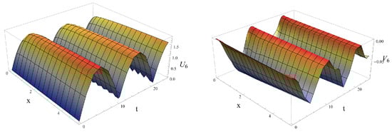
Figure 1. Profiles of the periodic traveling wave solutions $U_6(x,t)$ and $V_6(x,t)$ of (41) when $\alpha =0.3$, under $k=0.1,p\left(t\right)=2,a\left(t\right)={sin}^2\left(0.3t\right)$ and $c\left(t\right)=1$.

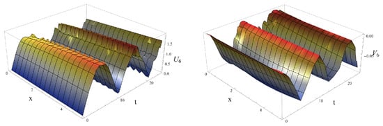
Figure 2. Profiles of the periodic traveling wave solutions $U_6(x,t)$ and $V_6(x,t)$ of (41) when $\alpha =0.8$, under $k=0.1,p\left(t\right)=2,a\left(t\right)={sin}^2\left(0.3t\right)$ and $c\left(t\right)=1$.

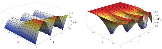
Figure 3. Profiles of the periodic traveling wave solution $U_6(x,t)$ and the solitons-like traveling wave solution $V_6(x,t)$ of (41) when $\alpha =1.0$, under $k=0.1,p\left(t\right)=2,a\left(t\right)={sin}^2\left(0.3t\right)$ and $c\left(t\right)=1$.

3.2. The Fractional WBK Equations with Variable Coefficients

Taking $f\left(U\right)=U,g\left(U_x^{\alpha }\right)=U_x^{\alpha },r\left(V\right)=V,a\left(t\right)=a\left(t\right),b\left(t\right)=b\left(t\right),c\left(t\right)=0$, we consider the fractional WBK equations with variable coefficients from Equation (2) in the form

$$\begin{array}{c}\hfill \left\{\begin{array}{c}\frac{{\partial }^{\alpha }V}{\partial t^{\alpha }}+\frac{{\partial }^{\alpha }}{\partial x^{\alpha }}\left(VU\right)+a\left(t\right)\frac{{\partial }^{3\alpha }U}{\partial x^{3\alpha }}-b\left(t\right)\frac{{\partial }^{2\alpha }V}{\partial x^{2\alpha }}=0,\hfill \\ \frac{{\partial }^{\alpha }U}{\partial t^{\alpha }}+\frac{{\partial }^{\alpha }V}{\partial x^{\alpha }}+U\frac{{\partial }^{\alpha }U}{\partial x^{\alpha }}+b\left(t\right)\frac{{\partial }^{2\alpha }U}{\partial x^{2\alpha }}=0.\hfill \end{array}\right.\end{array}$$

(42)

Suppose that $U(x,t)=\mathsf{u}\left(\zeta \right)$, $V(x,t)=\mathsf{v}\left(\zeta \right)$ are the fractional traveling wave solutions of Equation (42) where we applied the transformation given in Equation (4). With the use of traveling wave transformation (4), Equation (42) can be expressed by

$$\begin{array}{c}\hfill \left\{\begin{array}{c}-\omega \left(T\right){\mathsf{v}}^{\prime }+k{\mathsf{v}}^{\prime }\mathsf{u}+k\mathsf{v}{\mathsf{u}}^{\prime }+k^{3}a\left(t\right){\mathsf{u}}^{‴}-k^{2}b\left(t\right){\mathsf{v}}^{″}=0,\hfill \\ -\omega \left(T\right){\mathsf{u}}^{\prime }+k{\mathsf{v}}^{\prime }+k\mathsf{u}{\mathsf{u}}^{\prime }+k^{2}b\left(t\right){\mathsf{u}}^{″}=0,\hfill \end{array}\right.\end{array}$$

(43)

where ${\mathsf{u}}^{\prime }=d\mathsf{u}/d\zeta ,{\mathsf{u}}^{‴}=d^3\mathsf{u}/d{\zeta }^3,$${\mathsf{v}}^{\prime }=d\mathsf{v}/d\zeta ,{\mathsf{v}}^{″}=d^2\mathsf{v}/d{\zeta }^2.$

Integrating Equation (43) with respect to $\zeta$ once, we have

$$\begin{array}{c}\hfill \left\{\begin{array}{c}-\omega \left(T\right)\mathsf{v}+k\mathsf{v}\mathsf{u}+k^{3}a\left(t\right){\mathsf{u}}^{″}-k^{2}b\left(t\right){\mathsf{v}}^{\prime }=0,\hfill \\ -\omega \left(T\right)\mathsf{u}+k\mathsf{v}+\frac{1}{2}k{\mathsf{u}}^2+k^{2}b\left(t\right){\mathsf{u}}^{\prime }=0,\hfill \end{array}\right.\end{array}$$

(44)

From the second equation of Equation (44), we have

$$\begin{array}{c}\hfill \mathsf{v}=\frac{\omega \left(T\right)}{k}\mathsf{u}-\frac{1}{2}{\mathsf{u}}^2-kb\left(t\right){\mathsf{u}}^{\prime }.\end{array}$$

(45)

Substituting (45) into the first equation of Equation (44), we reduce Equation (44) to a single equation as follows:

$$\begin{array}{c}\hfill -{\omega }^2\left(T\right)\mathsf{u}+\frac{3}{2}k\omega \left(T\right){\mathsf{u}}^2-\frac{1}{2}{k}^2{\mathsf{u}}^3+k^4\left(a\left(t\right)+b^2\left(t\right)\right){\mathsf{u}}^{″}=0.\end{array}$$

(46)

By the homogeneous balancing principle, we take the highest-order nonlinear term ${\mathsf{u}}^3$ and the highest-order linear term ${\mathsf{u}}^{″}$ in Equation (46) for balancing, and we obtain the balanced order $M=1$, which satisfies $3M=M+2$. Then, Equation (46) has the first-order pole solution $\mathsf{u}\left(\zeta \right)$ as follows:

$$\begin{array}{c}\hfill \mathsf{u}\left(\zeta \right)=A_0\left(t\right)+A_1\left(t\right)\left[\frac{\psi \left(\zeta \right)}{\varphi \left(\zeta \right)}\right],\end{array}$$

(47)

and the solution $\mathsf{v}\left(\zeta \right)$ is simplifying in the second equation of Equation (44) as follows;

$$\begin{array}{c}\hfill \mathsf{v}\left(\zeta \right)=\frac{\omega \left(T\right)}{k}\mathsf{u}\left(\zeta \right)-\frac{1}{2}{\mathsf{u}}^2\left(\zeta \right)-kb\left(t\right){\mathsf{u}}^{\prime }\left(\zeta \right),\end{array}$$

(48)

where

$$\left[\frac{\psi \left(\zeta \right)}{\varphi \left(\zeta \right)}\right]=\frac{p\left(t\right)-q\left(t\right)}{p\left(t\right)-q\left(t\right)exp\{-(p\left(t\right)-q\left(t\right)\left)\zeta \right\}}.$$

and $\zeta =\zeta (x,t)=k{x}^{\alpha }/\alpha )-{\int }_0^T\omega \left(\tau \right)d\tau ,\tau ={\left[\alpha s\right]}^{1/\alpha },T=t^{\alpha }/\alpha$.

Substituting Expression (47) in Equation (46) and using improved System (6), we can obtain the algebraic equations by equating each coefficient of this polynomial in $\left[\psi \left(\zeta \right)/\varphi \left(\zeta \right)\right]$ to zero and solving the algebraic system by the help of Maple 2016, and we can find five nontrival sets of coefficients for the traveling wave solution $\mathsf{u}$ as follows:

$$\begin{array}{c}\hfill \left\{\begin{array}{c}\omega \left(t\right)=\pm 2k^{2}p\left(s\right)\sqrt{a\left(s\right)+b^2\left(s\right)},s={\left[t\alpha \right]}^{1/\alpha },q\left(t\right)=-p\left(t\right),\hfill \\ A_0\left(t\right)=0,A_1\left(t\right)=\pm 2kp\left(t\right)\sqrt{a\left(t\right)+b^2\left(t\right)},\hfill \end{array}\right.\end{array}$$

(49)

$$\begin{array}{c}\hfill \left\{\begin{array}{c}\omega \left(t\right)=\pm 2k^{2}p\left(s\right)\sqrt{a\left(s\right)+b^2\left(s\right)},s={\left[t\alpha \right]}^{1/\alpha },q\left(t\right)=-p\left(t\right),\hfill \\ A_0\left(t\right)=\pm 4kp\left(t\right)\sqrt{a\left(t\right)+b^2\left(t\right)},A_1\left(t\right)=\pm 2kp\left(t\right)\sqrt{a\left(t\right)+b^2\left(t\right)},\hfill \end{array}\right.\end{array}$$

(50)

$$\begin{array}{c}\hfill \left\{\begin{array}{c}\omega \left(t\right)=\pm 2k^{2}p\left(s\right)\sqrt{a\left(s\right)+b^2\left(s\right)},s={\left[t\alpha \right]}^{1/\alpha },q\left(t\right)=2p\left(t\right),\hfill \\ A_0\left(t\right)=0,A_1\left(t\right)=\pm 2kp\left(t\right)\sqrt{a\left(t\right)+b^2\left(t\right)},\hfill \end{array}\right.\end{array}$$

(51)

$$\begin{array}{c}\hfill \left\{\begin{array}{c}\omega \left(t\right)=\pm 2k^{2}p\left(s\right)\sqrt{a\left(s\right)+b^2\left(s\right)},s={\left[t\alpha \right]}^{1/\alpha },q\left(t\right)=2p\left(t\right),\hfill \\ A_0\left(t\right)=\pm 4kp\left(t\right)\sqrt{a\left(t\right)+b^2\left(t\right)},A_1\left(t\right)=\pm 2kp\left(t\right)\sqrt{a\left(t\right)+b^2\left(t\right)},\hfill \end{array}\right.\end{array}$$

(52)

$$\begin{array}{c}\hfill \left\{\begin{array}{c}\omega \left(t\right)=\pm k^{2}p\left(s\right)\sqrt{a\left(s\right)+b^2\left(s\right)},s={\left[t\alpha \right]}^{1/\alpha },q\left(t\right)=\frac{1}{2}p\left(t\right),\hfill \\ A_0\left(t\right)=\pm kp\left(t\right)\sqrt{a\left(t\right)+b^2\left(t\right)},A_1\left(t\right)=\pm 2kp\left(t\right)\sqrt{a\left(t\right)+b^2\left(t\right)},\hfill \end{array}\right.\end{array}$$

(53)

We can construct five coupled fractional traveling wave solutions by nontirivial coefficient sets (49)–(53) as follows. With a relation of $q\left(t\right)=-p\left(t\right)$, based on a coefficient set (49), the first coupled fractional traveling wave solutions of Equation (42) are expressed by

$$\begin{array}{c}\hfill \left\{\begin{array}{c}{U}_1(x,t)=\pm \frac{4kp\left(t\right)\sqrt{a\left(t\right)+b^2\left(t\right)}}{1+exp\{-2p\left(t\right){\zeta }_1(x,t)\}},\hfill \\ V_1(x,t)=-\frac{8k^2{p}^2\left(t\right)\left(a\left(t\right)+b^2\left(t\right)\right)}{{\left(1+exp\{-2p\left(t\right){\zeta }_1(x,t)\}\right)}^2}\mp \frac{8k^2{p}^2\left(t\right)b\left(t\right)\sqrt{a\left(t\right)+b^2\left(t\right)}exp\{-2p\left(t\right){\zeta }_1(x,t)\}}{{\left(1+exp\{-2p\left(t\right){\zeta }_1(x,t)\}\right)}^2}\pm \frac{4p\left(t\right)\omega \left(t\right)\sqrt{a\left(t\right)+b^2\left(t\right)}}{1+exp\{-2p\left(t\right){\zeta }_1(x,t)\}},\hfill \\ \omega \left(t\right)=\pm 2k^{2}p\left(s\right)\sqrt{a\left(s\right)+b^2\left(s\right)},s={\left[\alpha t\right]}^{1/\alpha },\hfill \end{array}\right.\end{array}$$

(54)

where ${\zeta }_1(x,t)=k{x}^{\alpha }/\alpha \mp {\int }_0^{T}2k^{2}p\left(s\right)\sqrt{a\left(s\right)+b^2\left(s\right)}d\tau$, $s={\left[\alpha \tau \right]}^{1/\alpha },$ and $T=t^{\alpha }/\alpha$. With a relation of $q\left(t\right)=-p\left(t\right)$, based on a coefficient set (50), the second coupled fractional traveling wave solutions of Equation (42) are written as

$$\begin{array}{c}\hfill \left\{\begin{array}{c}{U}_2(x,t)=\pm 4kp\left(t\right)\sqrt{a\left(t\right)+b^2\left(t\right)}\pm \frac{4kp\left(t\right)\sqrt{a\left(t\right)+b^2\left(t\right)}}{1+exp\{-2p\left(t\right){\zeta }_2(x,t)\}},\hfill \\ V_2(x,t)=\mp \frac{8k^2{p}^2\left(t\right)b\left(t\right)exp\left\{2p\left(t\right){\zeta }_2(x,t)\right\}}{{\left(1+exp\{-2p\left(t\right){\zeta }_2(x,t)\}\right)}^2}-\frac{1}{2}{\left(\pm 4kp\left(t\right)\sqrt{a\left(t\right)+b^2\left(t\right)}\pm \frac{4kp\left(t\right)\sqrt{a\left(t\right)+b^2\left(t\right)}}{1+exp\{-2p\left(t\right){\zeta }_2(x,t)\}}\right)}^2\hfill \\ +\frac{\omega \left(t\right)}{k}\left(\pm 4kp\left(t\right)\sqrt{a\left(t\right)+b^2\left(t\right)}\pm \frac{4kp\left(t\right)\sqrt{a\left(t\right)+b^2\left(t\right)}}{1+exp\{-2p\left(t\right){\zeta }_2(x,t)\}}\right),\hfill \\ \omega \left(t\right)=\pm 2k^{2}p\left(s\right)\sqrt{a\left(s\right)+b^2\left(s\right)},s={\left[\alpha t\right]}^{1/\alpha },\hfill \end{array}\right.\end{array}$$

(55)

where ${\zeta }_2(x,t)=k{x}^{\alpha }/\alpha \mp {\int }_0^{T}2k^{2}p\left(s\right)\sqrt{a\left(s\right)+b^2\left(s\right)}d\tau$, $s={\left[\alpha \tau \right]}^{1/\alpha },$ and $T=t^{\alpha }/\alpha$. With a relation of $q\left(t\right)=2p\left(t\right)$, based on a coefficient set (51), the third coupled fractional traveling wave solutions of Equation (42) are written as

$$\begin{array}{c}\hfill \left\{\begin{array}{c}{U}_3(x,t)=\mp \frac{2kp\left(t\right)\sqrt{a\left(t\right)+b^2\left(t\right)}}{1-2exp\left\{p\left(t\right){\zeta }_3(x,t)\right\}},\hfill \\ V_3(x,t)=-\frac{2k^2{p}^2\left(t\right)\left(a\left(t\right)+b^2\left(t\right)\right)}{{\left(1-2exp\left\{p\left(t\right){\zeta }_3(x,t)\right\}\right)}^2}\mp \frac{4k^2{p}^2\left(t\right)b\left(t\right)\sqrt{a\left(t\right)+b^2\left(t\right)}exp\left\{p\left(t\right){\zeta }_3(x,t)\right\}}{{\left(1-2exp\left\{p\left(t\right){\zeta }_3(x,t)\right\}\right)}^2}\pm \frac{2p\left(t\right)\omega \left(t\right)\sqrt{a\left(t\right)+b^2\left(t\right)}}{1-2exp\left\{p\left(t\right){\zeta }_3(x,t)\right\}},\hfill \\ \omega \left(t\right)=\pm 2k^{2}p\left(s\right)\sqrt{a\left(s\right)+b^2\left(s\right)},s={\left[\alpha t\right]}^{1/\alpha },\hfill \end{array}\right.\end{array}$$

(56)

where ${\zeta }_3(x,t)=k{x}^{\alpha }/\alpha \mp {\int }_0^{T}2k^{2}p\left(s\right)\sqrt{a\left(s\right)+b^2\left(s\right)}d\tau$, $s={\left[\alpha \tau \right]}^{1/\alpha },$ and $T=t^{\alpha }/\alpha$. With a relation of $q\left(t\right)=2p\left(t\right)$, based on a coefficient set (52), the fourth coupled fractional traveling wave solutions of Equation (42) are expressed by

$$\begin{array}{c}\hfill \left\{\begin{array}{c}{U}_4(x,t)=\pm 4kp\left(t\right)\sqrt{a\left(t\right)+b^2\left(t\right)}\mp \frac{2kp\left(t\right)\sqrt{a\left(t\right)+b^2\left(t\right)}}{1-2exp\left\{p\left(t\right){\zeta }_4(x,t)\right\}},\hfill \\ V_4(x,t)=\mp \frac{4k^2{p}^2\left(t\right)b\left(t\right)exp\left\{p\left(t\right){\zeta }_4(x,t)\right\}}{{\left(1-2exp\left\{p\left(t\right){\zeta }_4(x,t)\right\}\right)}^2}-\frac{1}{2}{\left(\pm 4kp\left(t\right)\sqrt{a\left(t\right)+b^2\left(t\right)}\mp \frac{2kp\left(t\right)\sqrt{a\left(t\right)+b^2\left(t\right)}}{1-2exp\left\{p\left(t\right){\zeta }_4(x,t)\right\}}\right)}^2\hfill \\ +\frac{\omega \left(t\right)}{k}\left(\pm 4kp\left(t\right)\sqrt{a\left(t\right)+b^2\left(t\right)}\mp \frac{2kp\left(t\right)\sqrt{a\left(t\right)+b^2\left(t\right)}}{1-2exp\left\{p\left(t\right){\zeta }_4(x,t)\right\}}\right),\hfill \\ \omega \left(t\right)=\pm 2k^{2}p\left(s\right)\sqrt{a\left(s\right)+b^2\left(s\right)},s={\left[\alpha t\right]}^{1/\alpha },\hfill \end{array}\right.\end{array}$$

(57)

where ${\zeta }_4(x,t)=k{x}^{\alpha }/\alpha \mp {\int }_0^{T}2k^{2}p\left(s\right)\sqrt{a\left(s\right)+b^2\left(s\right)}d\tau$, $s={\left[\alpha \tau \right]}^{1/\alpha },$ and $T=t^{\alpha }/\alpha$. With a relation of $q\left(t\right)=\frac{1}{2}p\left(t\right)$, based on a coefficient set (53), the last coupled fractional traveling wave solutions of Equation (42) are given by

$$\begin{array}{c}\hfill \left\{\begin{array}{c}{U}_5(x,t)=\pm kp\left(t\right)\sqrt{a\left(t\right)+b^2\left(t\right)}\pm \frac{2kp\left(t\right)\sqrt{a\left(t\right)+b^2\left(t\right)}}{2-exp\{-\frac{1}{2}p\left(t\right){\zeta }_5(x,t)\}},\hfill \\ V_5(x,t)=\mp \frac{k^2{p}^2\left(t\right)b\left(t\right)exp\{-\frac{1}{2}p\left(t\right){\zeta }_5(x,t)\}}{2{\left(2-exp\{-\frac{1}{2}p\left(t\right){\zeta }_5(x,t)\}\right)}^2}-\frac{1}{2}{\left(\pm kp\left(t\right)\sqrt{a\left(t\right)+b^2\left(t\right)}\pm \frac{2kp\left(t\right)\sqrt{a\left(t\right)+b^2\left(t\right)}}{2-exp\{-\frac{1}{2}p\left(t\right){\zeta }_5(x,t)\}}\right)}^2\hfill \\ +\frac{\omega \left(t\right)}{k}\left(\pm kp\left(t\right)\sqrt{a\left(t\right)+b^2\left(t\right)}\pm \frac{2kp\left(t\right)\sqrt{a\left(t\right)+b^2\left(t\right)}}{2-exp\{-\frac{1}{2}p\left(t\right){\zeta }_5(x,t)\}}\right),\hfill \\ \omega \left(t\right)=\pm k^{2}p\left(s\right)\sqrt{a\left(s\right)+b^2\left(s\right)},s={\left[\alpha t\right]}^{1/\alpha },\hfill \end{array}\right.\end{array}$$

(58)

where ${\zeta }_5(x,t)=k{x}^{\alpha }/\alpha \mp {\int }_0^T{k}^{2}p\left(s\right)\sqrt{a\left(s\right)+b^2\left(s\right)}d\tau$, $s={\left[\alpha \tau \right]}^{1/\alpha },$ and $T=t^{\alpha }/\alpha$.

We represent the dynamics of the coupled fractional traveling wave solution (4) with fractional orders as follows; Figure 4, Figure 5 and Figure 6 represent the periodic traveling wave behaviors of the fractional traveling wave solutions $U_5(x,t)$ and $V_5(x,t)$ of (58) with fractional orders $\alpha =0.3,0.8,1.0$, under $k=0.1,p\left(t\right)=1.2,a\left(t\right)=sin\left(0.5t\right)$ and $b\left(t\right)=1$.

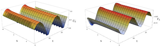
Figure 4. Profiles of the periodic traveling wave solutions $U_5(x,t)$ and $V_5(x,t)$ of (58) when $\alpha =0.3$, under $k=0.1,p\left(t\right)=1.2,a\left(t\right)=sin\left(0.5t\right)$ and $b\left(t\right)=1$.

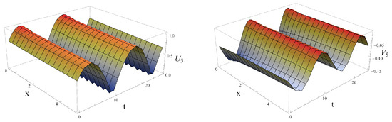
Figure 5. Profiles of the periodic traveling wave solutions $U_5(x,t)$ and $V_5(x,t)$ of (58) when $\alpha =0.8$, under $k=0.1,p\left(t\right)=1.2,a\left(t\right)=sin\left(0.5t\right)$ and $b\left(t\right)=1$.

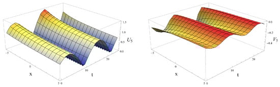
Figure 6. Profiles of the periodic traveling wave solutions $U_5(x,t)$ and $V_5(x,t)$ of (58) when $\alpha =1.0$, under $k=0.1,p\left(t\right)=1.2,a\left(t\right)=sin\left(0.5t\right)$ and $b\left(t\right)=1$.

Remark 1.

For the integral order $\alpha =1$, if $A\left(t\right)=a$ and $B\left(t\right)=b$ are constants, Equation (42) gives the WBK equations as follows:

$$\begin{array}{c}\hfill \left\{\begin{array}{c}{v}_t+{\left(uv\right)}_x+a{u}_{xxx}-b{v}_{xx}=0,\hfill \\ u_t+v_x+u{u}_x+b{u}_{xx}=0,\hfill \end{array}\right.\end{array}$$

(59)

where $u(x,t)$ and $v(x,t)$ are described as the dispersive long-wave in shallow water waves, as $u(x,t)$ is the field of horizontal velocity and $v(x,t)$ represents the height that deviates from the equilibrium position of liquid, and a and b represent different diffusion powers [6,26,27]. Especially, if we take $a=0$ and $b\ne 0$, Equation (59) has five coupled traveling wave solutions of the classic long wave equations as follows:

$$\begin{array}{c}\hfill \left\{\begin{array}{c}{u}_1(x,t)=\pm \frac{4kp\left(t\right)\left|b\right|}{1+exp\{-2p(t\left)\zeta \right(x,t\left)\right\}},\hfill \\ v_1(x,t)=\frac{8k^2{p}^2\left(t\right)\left[b\left(b\mp \left|b\right|\right)\right]exp\left\{2p\left(t\right)\zeta (x,t)\right\}}{{(1+exp\left\{2p\left(t\right)\zeta (x,t)\right\})}^2},\hfill \end{array}\right.\end{array}$$

(60)

$$\begin{array}{c}\hfill \left\{\begin{array}{c}{u}_2(x,t)=\pm 4kp\left(t\right)\left|b\right|\pm \frac{4kp\left(t\right)\left|b\right|}{1+exp\{-2p(t\left)\zeta \right(x,t\left)\right\}},\hfill \\ v_2(x,t)=-\frac{8k^2{p}^2\left(t\right)\left[b^2\pm b\left|b\right|+2b^{2}exp\left\{2p\left(t\right)\zeta (x,t)\right\}\right]exp\left\{2p\left(t\right)\zeta (x,t)\right\}}{{(1+exp\left\{2p\left(t\right)\zeta (x,t)\right\})}^2},\hfill \end{array}\right.\end{array}$$

(61)

$$\begin{array}{c}\hfill \left\{\begin{array}{c}{u}_3(x,t)=\mp \frac{2kp\left(t\right)\left|b\right|}{1-2exp\left\{p\right(t\left)\zeta \right(x,t\left)\right\}},\hfill \\ v_3(x,t)=\frac{2k{p}^2\left(t\right)\left[b^2\left(3-4exp\left\{p\right(t\left)\zeta \right(x,t\left)\right\}\right)\mp 2b\left|b\right|exp\left\{p\left(t\right)\zeta (x,t)\right\}\right]}{{\left(1-2exp\left\{p\right(t\left)\zeta \right(x,t\left)\right\}\right)}^2},\hfill \end{array}\right.\end{array}$$

(62)

$$\begin{array}{c}\hfill \left\{\begin{array}{c}{u}_4(x,t)=\pm 4kp\left(t\right)\left|b\right|\mp \frac{2kp\left(t\right)\left|b\right|}{1-2exp\left\{p\right(t\left)\zeta \right(x,t\left)\right\}},\hfill \\ v_4(x,t)=\frac{2k^2{p}^2\left(t\right)\left[b^2-\left(4b^2\pm 2b\left|b\right|\right)exp\left\{p\left(t\right)\zeta (x,t)\right\}\right]}{{\left(1-2exp\left\{p\right(t\left)\zeta \right(x,t\left)\right\}\right)}^2},\hfill \end{array}\right.\end{array}$$

(63)

where $\zeta (x,t)=kx\mp {\int }_0^{t}2k^{2}p\left(s\right)\left|b\right|ds$,

$$\begin{array}{c}\hfill \left\{\begin{array}{c}{u}_5(x,t)=\pm kp\left(t\right)\left|b\right|\pm \frac{2kp\left(t\right)\left|b\right|}{2-exp\{-\frac{1}{2}p\left(t\right){\zeta }_5(x,t)\}},\hfill \\ v_5(x,t)=\frac{k^2{p}^2\left(t\right)\left[b^2\left(1-4exp\left\{\frac{1}{2}p\left(t\right){\zeta }_5(x,t)\right\}\right)\pm 2b\left|b\right|exp\left\{\frac{1}{2}p\left(t\right){\zeta }_5(x,t)\right\}\right]}{2{\left(1-2exp\{\frac{1}{2}p\left(t\right){\zeta }_5(x,t)\right)}^2},\hfill \end{array}\right.\end{array}$$

(64)

where ${\zeta }_5(x,t)=kx\mp {\int }_0^t{k}^{2}p\left(s\right)\left|b\right|ds$.

3.3. The Fractional Boussinesq Equations with Variable Coefficients

By setting $f\left(U\right)=U,g\left(U_x^{\alpha }\right)=U_x^{\alpha },r\left(V\right)=V,a\left(t\right)=a\left(t\right),b\left(t\right)=0,c\left(t\right)=0$ in Equation (2), the fractional Boussinesq equations with variable coefficients are degenerated as in the form [28]

$$\begin{array}{c}\hfill \left\{\begin{array}{c}\frac{{\partial }^{\alpha }V}{\partial t^{\alpha }}+\frac{{\partial }^{\alpha }}{\partial x^{\alpha }}\left(VU\right)+a\left(t\right)\frac{{\partial }^{3\alpha }u}{\partial x^{3\alpha }}=0,\hfill \\ \frac{{\partial }^{\alpha }U}{\partial t^{\alpha }}+\frac{{\partial }^{\alpha }V}{\partial x^{\alpha }}+U\frac{{\partial }^{\alpha }U}{\partial x^{\alpha }}=0.\hfill \end{array}\right.\end{array}$$

(65)

Suppose that $U(x,t)=\mathsf{u}\left(\eta \right)$, $V(x,t)=\mathsf{v}\left(\eta \right)$ are the fractional traveling wave solutions of Equation (65) with the fractional traveling wave varaible $\eta =k{x}^{\alpha }/\alpha -{\int }_0^T\omega \left(s\right)ds$, $T=t^{\alpha }/\alpha$, where k is an arbitrary constant and $\alpha \in (0,1]$. Then, Equation (65) can be written by

$$\begin{array}{c}\hfill \left\{\begin{array}{c}-\omega \left(T\right){\mathsf{v}}^{\prime }+k{\mathsf{v}}^{\prime }\mathsf{u}+k\mathsf{v}{\mathsf{u}}^{\prime }+k^{3}a\left(t\right){\mathsf{u}}^{‴}=0,\hfill \\ -\omega \left(T\right){\mathsf{u}}^{\prime }+k{\mathsf{v}}^{\prime }+k\mathsf{u}{\mathsf{u}}^{\prime }=0,\hfill \end{array}\right.\end{array}$$

(66)

where ${\mathsf{u}}^{\prime }=d\mathsf{u}/d\zeta ,{\mathsf{u}}^{‴}=d^3\mathsf{u}/d{\zeta }^3,$${\mathsf{v}}^{\prime }=d\mathsf{v}/d\zeta .$

Integrating Equation (66) with respect to $\zeta$ once, we have

$$\begin{array}{c}\hfill \left\{\begin{array}{c}-\omega \left(T\right)\mathsf{v}+k\mathsf{v}\mathsf{u}+k^{3}a\left(t\right){\mathsf{u}}^{″}=0,\hfill \\ -\omega \left(T\right)\mathsf{u}+k\mathsf{v}+\frac{1}{2}k{\mathsf{u}}^2=0.\hfill \end{array}\right.\end{array}$$

(67)

From the second equation of Equation (67), we have

$$\begin{array}{c}\hfill \mathsf{v}=\frac{\omega \left(T\right)}{k}\mathsf{u}-\frac{1}{2}{\mathsf{u}}^2.\end{array}$$

(68)

Substituting (68) into the first equation of Equation (67), we reduce Equation (67) to a single equation as follows:

$$\begin{array}{c}\hfill -{\omega }^2\left(T\right)\mathsf{u}+\frac{3}{2}k\omega \left(T\right){\mathsf{u}}^2-\frac{1}{2}{k}^2{\mathsf{u}}^3+k^{4}a\left(t\right){\mathsf{u}}^{″}=0.\end{array}$$

(69)

We know that Equation (69) has the first-order pole solution $\mathsf{u}\left(\zeta \right)$ by the homogeneous balancing principle. Then, we suppose that the solution of Equation (69) can be expressed in the form

$$\begin{array}{c}\hfill \mathsf{u}\left(\zeta \right)=A_0\left(t\right)+A_1\left(t\right)\frac{p\left(t\right)-q\left(t\right)}{p\left(t\right)-q\left(t\right)exp\{-(p\left(t\right)-q\left(t\right)\left)\zeta \right\}},\end{array}$$

(70)

and the solution $\mathsf{v}\left(\zeta \right)$ is expressed by in the form

$$\begin{array}{c}\hfill \mathsf{v}\left(\zeta \right)=\frac{\omega \left(T\right)}{k}\mathsf{u}\left(\zeta \right)-\frac{1}{2}{\mathsf{u}}^2\left(\zeta \right).\end{array}$$

(71)

We have the coupled fractional traveling wave solutions of Equation (65) as follows:

$$\begin{array}{c}\hfill \left\{\begin{array}{c}{U}_1(x,t)=\pm \frac{4kp\left(t\right)\sqrt{a\left(t\right)}}{1+exp\{-2p\left(t\right){\zeta }_1(x,t)\}},\hfill \\ V_1(x,t)=-\frac{8k^2{p}^2\left(t\right)a\left(t\right)}{{\left(1+exp\{-2p\left(t\right){\zeta }_1(x,t)\}\right)}^2}\pm \frac{4p^2\left(t\right)\omega \left(t\right)\sqrt{a\left(t\right)}}{1+exp\{-2p\left(t\right){\zeta }_1(x,t)\}},\hfill \\ \omega \left(t\right)=\pm 2k^{2}p\left(s\right)\sqrt{a\left(s\right)},s={\left[\alpha t\right]}^{1/\alpha },\hfill \end{array}\right.\end{array}$$

(72)

where ${\zeta }_1(x,t)=k{x}^{\alpha }/\alpha \mp {\int }_0^{T}2k^{2}p\left(s\right)\sqrt{a\left(s\right)}d\tau$, $s={\left[\alpha \tau \right]}^{1/\alpha },$ and $T=t^{\alpha }/\alpha$, with $q\left(t\right)=-p\left(t\right)$,

$$\begin{array}{c}\hfill \left\{\begin{array}{c}{U}_2(x,t)=\pm 4kp\left(t\right)\sqrt{a\left(t\right)}\pm \frac{4kp\left(t\right)\sqrt{a\left(t\right)}}{1+exp\{-2p\left(t\right){\zeta }_2(x,t)\}},\hfill \\ V_2(x,t)=-\frac{1}{2}{\left(\pm 4kp\left(t\right)\sqrt{a\left(t\right)}\pm \frac{4kp\left(t\right)\sqrt{a\left(t\right)}}{1+exp\{-2p\left(t\right){\zeta }_2(x,t)\}}\right)}^2\hfill \\ +\frac{\omega \left(t\right)}{k}\left(\pm 4kp\left(t\right)\sqrt{a\left(t\right)}\pm \frac{4kp\left(t\right)\sqrt{a\left(t\right)}}{1+exp\{-2p\left(t\right){\zeta }_2(x,t)\}}\right),\hfill \\ \omega \left(t\right)=\pm 2k^{2}p\left(s\right)\sqrt{a\left(s\right)},s={\left[\alpha t\right]}^{1/\alpha },\hfill \end{array}\right.\end{array}$$

(73)

where ${\zeta }_2(x,t)=k{x}^{\alpha }/\alpha \mp {\int }_0^{T}2k^{2}p\left(s\right)\sqrt{a\left(s\right)}d\tau$, $s={\left[\alpha \tau \right]}^{1/\alpha },$ and $T=t^{\alpha }/\alpha$, with $q\left(t\right)=-p\left(t\right)$,

$$\begin{array}{c}\hfill \left\{\begin{array}{c}{U}_3(x,t)=\mp \frac{2kp\left(t\right)\sqrt{a\left(t\right)}}{1-2exp\left\{p\left(t\right){\zeta }_3(x,t)\right\}},\hfill \\ V_3(x,t)=-\frac{2k^2{p}^2\left(t\right)a\left(t\right)}{{\left(1-2exp\left\{p\left(t\right){\zeta }_3(x,t)\right\}\right)}^2}\mp \frac{2p^2\left(t\right)\omega \left(t\right)\sqrt{a\left(t\right)}}{1-2exp\left\{p\left(t\right){\zeta }_3(x,t)\right\}},\hfill \\ \omega \left(t\right)=\pm 2k^{2}p\left(s\right)\sqrt{a\left(s\right)},s={\left[\alpha t\right]}^{1/\alpha },\hfill \end{array}\right.\end{array}$$

(74)

where ${\zeta }_3(x,t)=k{x}^{\alpha }/\alpha \mp {\int }_0^{T}2k^{2}p\left(s\right)\sqrt{a\left(s\right)}d\tau$, $s={\left[\alpha \tau \right]}^{1/\alpha },$ and $T=t^{\alpha }/\alpha$, with $q\left(t\right)=2p\left(t\right)$,

$$\begin{array}{c}\hfill \left\{\begin{array}{c}{U}_4(x,t)=\pm 4kp\left(t\right)\sqrt{a\left(t\right)}\mp \frac{2kp\left(t\right)\sqrt{a\left(t\right)}}{1-2exp\left\{p\left(t\right){\zeta }_4(x,t)\right\}},\hfill \\ V_4(x,t)=-\frac{1}{2}{\left(\pm 4kp\left(t\right)\sqrt{a\left(t\right)}\mp \frac{2kp\left(t\right)\sqrt{a\left(t\right)}}{1-2exp\left\{p\left(t\right){\zeta }_4(x,t)\right\}}\right)}^2\hfill \\ +\frac{\omega \left(t\right)}{k}\left(\pm 4kp\left(t\right)\sqrt{a\left(t\right)}\mp \frac{2kp\left(t\right)\sqrt{a\left(t\right)}}{1-2exp\left\{p\left(t\right){\zeta }_4(x,t)\right\}}\right),\hfill \\ \omega \left(t\right)=\pm 2k^{2}p\left(s\right)\sqrt{a\left(s\right)},s={\left[\alpha t\right]}^{1/\alpha },\hfill \end{array}\right.\end{array}$$

(75)

where ${\zeta }_4(x,t)=k{x}^{\alpha }/\alpha \mp {\int }_0^{T}2k^{2}p\left(s\right)\sqrt{a\left(s\right)}d\tau$, $s={\left[\alpha \tau \right]}^{1/\alpha },$ and $T=t^{\alpha }/\alpha$, with $q\left(t\right)=2p\left(t\right)$,

$$\begin{array}{c}\hfill \left\{\begin{array}{c}{U}_5(x,t)=\pm kp\left(t\right)\sqrt{a\left(t\right)}\pm \frac{2kp\left(t\right)\sqrt{a\left(t\right)}}{2-exp\{-\frac{1}{2}p\left(t\right){\zeta }_5(x,t)\}},\hfill \\ V_5(x,t)=-\frac{1}{2}{\left(\pm kp\left(t\right)\sqrt{a\left(t\right)}\pm \frac{2kp\left(t\right)\sqrt{a\left(t\right)}}{2-exp\{-\frac{1}{2}p\left(t\right){\zeta }_5(x,t)\}}\right)}^2\hfill \\ +\frac{\omega \left(t\right)}{k}\left(\pm kp\left(t\right)\sqrt{a\left(t\right)}\pm \frac{2kp\left(t\right)\sqrt{a\left(t\right)}}{2-exp\{-\frac{1}{2}p\left(t\right){\zeta }_5(x,t)\}}\right),\hfill \\ \omega \left(t\right)=\pm k^{2}p\left(s\right)\sqrt{a\left(s\right)},s={\left[\alpha t\right]}^{1/\alpha },\hfill \end{array}\right.\end{array}$$

(76)

where ${\zeta }_5(x,t)=k{x}^{\alpha }/\alpha \mp {\int }_0^T{k}^{2}p\left(s\right)\sqrt{a\left(s\right)}d\tau$, $s={\left[\alpha \tau \right]}^{1/\alpha },$ and $T=t^{\alpha }/\alpha$, with $q\left(t\right)=p\left(t\right)/2$.

We illustrate the dynamics of the coupled fractional traveling wave solution (76) with fractional orders as follows: Figure 7, Figure 8 and Figure 9 represent the solitary wave behaviors of the fractional traveling wave solutions $U_5(x,t)$ and $V_5(x,t)$ of (76) with fractional orders $\alpha =0.3,0.8,1.0$, under $k=0.25,p\left(t\right)=exp(-t/3),a\left(t\right)={sin}^2\left(0.5t\right)$: for fractional orders $\alpha =0.3,0.8,1.0$, the fractional traveling wave solutions $U_5(x,t)$ and $V_5(x,t)$ of (76) converge to 0 as time variable t increases for all space variable x.

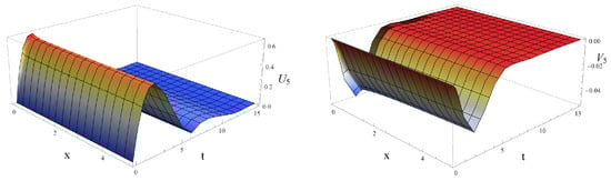
Figure 7. Profiles of the solitary wave solution $U_5(x,t)$ and the dark solitary wave solution $V_5(x,t)$ of (76) when $\alpha =0.3$, under $k=0.25,p\left(t\right)=exp(-t/3),a\left(t\right)={sin}^2\left(0.5t\right)$.

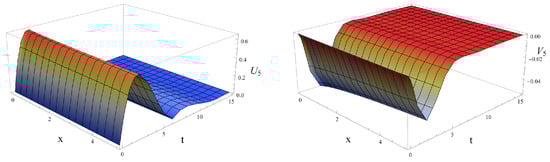
Figure 8. Profiles of the solitary wave solution $U_5(x,t)$ and the dark solitary wave solution $V_5(x,t)$ of (76) when $\alpha =0.8$, under $k=0.25,p\left(t\right)=exp(-t/3),a\left(t\right)={sin}^2\left(0.5t\right)$.

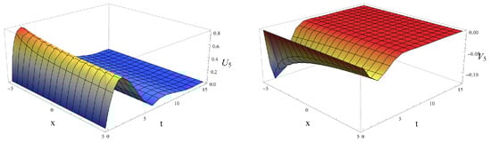
Figure 9. Profiles of the solitary wave solution $U_5(x,t)$ and the dark solitary wave solution $V_5(x,t)$ of (76) when $\alpha =1.0$, under $k=0.25,p\left(t\right)=exp(-t/3),a\left(t\right)={sin}^2\left(0.5t\right)$.

Remark 2.

When we take the interger order $\alpha =1$ and $a\left(t\right)=1$, the version of Equation (65) is expressed by

$$\begin{array}{c}\hfill \left\{\begin{array}{c}{\mathsf{v}}_t+{\left(\mathsf{u}\mathsf{v}\right)}_x+{\mathsf{u}}_{xxx}=0,\hfill \\ {\mathsf{u}}_t+{\mathsf{v}}_x+\mathsf{u}{\mathsf{u}}_x=0,\hfill \end{array}\right.\end{array}$$

(77)

which is called the Boussinesq I equations [29,30]. By employing mathematical computation method, we obtain the coupled traveling wave solutions of Equation (77) as follows:

$$\begin{array}{c}\hfill \left\{\begin{array}{c}{u}_1(x,t)=\pm \frac{4kp\left(t\right)}{1+exp\{-2p(t\left)\zeta \right(x,t\left)\right\}},\hfill \\ v_1(x,t)=-\frac{8k^2{p}^2\left(t\right)exp\left\{2p\left(t\right)\zeta (x,t)\right\}}{{\left(1+exp\left\{2p\right(t\left)\zeta \right(x,t\left)\right\}\right)}^2},\hfill \end{array}\right.\end{array}$$

(78)

$$\begin{array}{c}\hfill \left\{\begin{array}{c}{u}_2(x,t)=\pm 4kp\left(t\right)\pm \frac{4kp\left(t\right)}{1+exp\{-2p(t\left)\zeta \right(x,t\left)\right\}},\hfill \\ v_2(x,t)=\frac{8k{p}^2\left(t\right)exp\left\{2p\left(t\right)\zeta (x,t)\right\}}{{\left(1+exp\left\{2p\right(t\left)\zeta \right(x,t\left)\right\}\right)}^2},\hfill \end{array}\right.\end{array}$$

(79)

$$\begin{array}{c}\hfill \left\{\begin{array}{c}{u}_3(x,t)=\mp \frac{2kp\left(t\right)}{1-2exp\left\{p\right(t\left)\zeta \right(x,t\left)\right\}},\hfill \\ v_3(x,t)=\frac{2k^2{p}^2\left(t\right)\left(1-4exp\left\{p\right(t\left)\zeta \right(x,t\left)\right\}\right)}{{\left(1-2exp\left\{p\right(t\left)\zeta \right(x,t\left)\right\}\right)}^2},\hfill \end{array}\right.\end{array}$$

(80)

$$\begin{array}{c}\hfill \left\{\begin{array}{c}{u}_4(x,t)=\pm 4kp\left(t\right)\mp \frac{2kp\left(t\right)}{1-2exp\left\{p\right(t\left)\zeta \right(x,t\left)\right\}},\hfill \\ v_4(x,t)=\frac{2k^2{p}^2\left(t\right)\left(1-4exp\left\{p\right(t\left)\zeta \right(x,t\left)\right\}\right)}{{\left(1-2exp\left\{p\right(t\left)\zeta \right(x,t\left)\right\}\right)}^2},\hfill \end{array}\right.\end{array}$$

(81)

where $\zeta (x,t)=kx\mp {\int }_0^{t}2k^{2}p\left(s\right)ds$,

$$\begin{array}{c}\hfill \left\{\begin{array}{c}{u}_5(x,t)=\pm kp\left(t\right)\pm \frac{2kp\left(t\right)}{2-exp\{-\frac{1}{2}p\left(t\right){\zeta }_5(x,t)\}},\hfill \\ v_5(x,t)=\frac{k^2{p}^2\left(t\right)\left(1-4exp\left\{\frac{1}{2}p\left(t\right){\zeta }_5(x,t)\right\}\right)}{2{\left(1-2exp\left\{\frac{1}{2}p\left(t\right){\zeta }_5(x,t)\right\}\right)}^2},\hfill \end{array}\right.\end{array}$$

(82)

where ${\zeta }_5(x,t)=kx\mp {\int }_0^t{k}^{2}p\left(s\right)ds$.

4. Conclusions

In this paper, we obtained new coupled fractional traveling wave solutions of the fractional BWBK equations, the fractional WBK equations and the fractional Boussinesq equations with variable coefficients by using the improved system method. We have successfully applied the improved system method to find new coupled fractional traveling wave solutions of the fractional NPDEs. We presented the dynamics of new coupled fractional traveling wave solutions of the considered equations under suitable physical parameters. We believe that the improved system method is simple and powerful to find the explicit traveling wave solutions of NPDEs.

References

- Klopman, G.; Van Groesen, E.; Dingemans, M.W. A variational approach to Boussinesq modelling of fully nonlinear water waves. J. Fluid Mech. 2010, 657, 36–63. [Google Scholar] [CrossRef]
- Lawrence, C.; Adytia, D.; Van Groesen, E. Variational Boussinesq model for strongly nonlinear dispersive waves. Wave Motion 2017, 76. [Google Scholar] [CrossRef]
- Khan, K.; Akbar, M.A. Study of analytical method to seek for exact solutions of variant Boussinesq equations. Springer Plus 2014, 3, 324. Available online: http://www.springerplus.com/content/3/1/324 (accessed on 27 June 2014). [CrossRef] [Green Version]
- Wang, M.; Li, X.; Zhang, J. The (G′/G)-expansion method and travelling wave solutions of nonlinear evolution equations in mathematical physics. Phys. Lett. A 2008, 372, 417–423. [Google Scholar] [CrossRef]
- Abazari, R.; Jamshidzadeh, S.; Biswas, A. Solitary wave solutions of coupled Boussinesq equation. Complexity 2016, 21, 151–155. [Google Scholar] [CrossRef]
- Tian, B.; Qiu, Y. Exact and Explicit Solutions of Whitham-Broer-Kaup Equations in Shallow Water. Pure Appl. Math. J. 2016, 5, 174–180. [Google Scholar] [CrossRef] [Green Version]
- Zhang, Z.; Yong, X.; Chen, Y. Symmetry analysis for Whitham-Broer-Kaup equations. J. Nonlinear Math. Phys. 2008, 15, 383–397. [Google Scholar] [CrossRef] [Green Version]
- Mohyud-Din, S.T.; Yıldırım, A.; Demirli, G. Traveling wave solutions of Whitham–Broer–Kaup equations by homotopy perturbation method. J. King Saud Univ. Sci. 2010, 22, 173–176. [Google Scholar] [CrossRef] [Green Version]
- Xie, F.D.; Yan, Z.Y.; Zhang, H.Q. Explicit and exact traveling wave solutions of Whitham-Broer-Kaup shallow water equations. Phys. Lett. A 2001, 285, 76–80. [Google Scholar] [CrossRef]
- El-sayed, S.M.; Kaya, D. Exact and numerical traveling wave solutions of Whitham-Broer-Kaup equations. Appl. Math. Comput. 2005, 167, 1339–1349. [Google Scholar] [CrossRef]
- Yang, X.-F.; Deng, Z.-C.; Lib, Q.-J.; Wei, Y. Exact combined traveling wave solutions and multi-symplectic structure of the variant Boussinesq-Whitham-Broer-Kaup type equations. Commun. Nonliner Sci. Numer. Simul. 2016, 36, 1–13. [Google Scholar] [CrossRef]
- Atangana, A.; Alqahtani, R.T. Modelling the spread of river blindness disease via the Caputo Fractional Derivative and the Beta-derivative. Entrophy 2016, 18, 40. [Google Scholar] [CrossRef]
- Atangana, A.; Goufo, E.F.D. Extension of mathced asymtotic method to fractional boundary layers problems. Math. Probl. Eng. 2014, 2014, 107535. [Google Scholar] [CrossRef] [Green Version]
- Liang, J.; Tang, L.; Xia, Y.; Zhang, Y. Bifurcations and Exact Solutions for a Class of MKdV Equations with the Conformable Fractional Derivative via Dynamical System Method. Int. J. Bifurc. Chaos 2020, 30, 2050004. [Google Scholar] [CrossRef]
- Gao, F.; Chi, C. Improvement on Conformable Fractional Derivative and Its Applications in Fractional Differential Equations. J. Funct. Spac. 2020, 2020, 5852414. [Google Scholar] [CrossRef]
- Korpina, Z.; Tchier, F.; Bousbahi, F.; Tawfiq, F.; AliAkinlar, M. Applicability of time conformable derivative to Wick-fractional-stochastic PDEs. Alexandria Eng. J. 2020, 59, 1485–1493. [Google Scholar] [CrossRef]
- Choi, J.H.; Kim, H. Exact traveling wave solutions of the stochastic Wick-type fractional Caudrey-Dodd-Gibbon-Sawada-Kotera equation. AIMS Math. 2021, 6, 4053–4072. [Google Scholar] [CrossRef]
- Kim, H.; Sakthivel, R.; Debbouche, A.; Torres, D.F.M. Traveling wave solutions of some important Wick-type fractional stochastic nonlinear partial differential equations. Chaos Solitons Fractals 2020, 131, 109542. [Google Scholar] [CrossRef] [Green Version]
- Choi, J.H.; Kim, H.; Sakthivel, R. Periodic and solitary wave solutions of some important physical models with variable coefficients. Waves Random Complex Media 2019. [Google Scholar] [CrossRef]
- Choi, J.H.; Lee, S.; Kim, H. Stochastic Effects for the Reaction-Duffing Equation with Wick-Type Product. Adv. Math. Phys. 2016, 2016. [Google Scholar] [CrossRef]
- Kim, H.; Lee, S. Explicit solutions of the fifth-order KdV type nonlinear evolution equation using the system technique. Results Phys. 2016, 6, 992–997. [Google Scholar] [CrossRef] [Green Version]
- Wang, M.; Zhou, Y.; Li, Z. Application of a Homogeneous Balance Method to Exact Solutions of Nonlinear Equations in Mathematical Physics. Phys. Lett. A 1996, 216, 67–75. [Google Scholar] [CrossRef]
- Wang, M.L. Exact solutions for a compound KdV-Burgers equation. Phys. Lett. A 1996, 213, 279–287. [Google Scholar] [CrossRef]
- Ablowitz, M.J.; Ramani, A.; Segar, H. A connection between nonlinear evolution equations and ordinary differential equations of P-type. I. J. Math. Phys. 1980, 21, 715–721. [Google Scholar] [CrossRef]
- Ablowitz, M.J.; Ramani, A.; Segar, H. A connection between nonlinear evolution equations and ordinary differential equations of P-type. II. J. Math. Phys. 1980, 21, 1006–1015. [Google Scholar] [CrossRef]
- Kupershmidt, B.A. Mathematics of Dispersive Water Waves. Commun. Math. Phys. 1985, 99, 51–73. [Google Scholar] [CrossRef]
- Lin, J.; Xu, Y.-S.; Wu, F.-M. Evolution property of soliton solutions for the Whitham-Broer-Kaup equation and variant Boussinesq equation. Chin. Phys. 2003, 12, 1049–1053. [Google Scholar]
- Fan, E.; Hon, Y.C. A series of traveling wave solutions for the two variant Boussinesq equations in shallow water waves. Chaos Solitons Fractals 2003, 15, 559–566. [Google Scholar] [CrossRef]
- Sachs, R.L. On the integrable variant of the Boussinesq system: Painlevé property, rational solutions, a related many-body system, and equivalence with the AKNS hierarchy. Physica D 1998, 30, 1–27. [Google Scholar] [CrossRef]
- Zayed, E.M.E.; Ai-Nowehy, A.G. Solitons and the exact solutions for variant nonlinear Boussinesq equations. Optik 2017, 139, 166–177. [Google Scholar] [CrossRef]
Publisher’s Note: MDPI stays neutral with regard to jurisdictional claims in published maps and institutional affiliations. |
© 2021 by the authors. Licensee MDPI, Basel, Switzerland. This article is an open access article distributed under the terms and conditions of the Creative Commons Attribution (CC BY) license (https://creativecommons.org/licenses/by/4.0/).