Exact Time-Dependent Solutions and Information Geometry of a Rocking Ratchet

Abstract

The noise-induced transport due to spatial symmetry-breaking is a key mechanism for the generation of a uni-directional motion by a Brownian motor. By utilising an asymmetric sawtooth periodic potential and three different types of periodic forcing $G\left(t\right)$ (sinusoidal, square and sawtooth waves) with period T and amplitude A, we investigate the performance (energetics, mean current, Stokes efficiency) of a rocking ratchet in light of thermodynamic quantities (entropy production) and the path-dependent information geometric measures. For each $G\left(t\right)$, we calculate exact time-dependent probability density functions under different conditions by varying T, A and the strength of the stochastic noise D in an unprecedentedly wide range. Overall similar behaviours are found for different cases of $G\left(t\right)$. In particular, in all cases, the current, Stokes efficiency and the information rate normalised by A and D exhibit one or multiple local maxima and minima as A increases. However, the dependence of the current and Stokes efficiency on A can be quite different, while the behaviour of the information rate normalised by A and D tends to resemble that of the Stokes efficiency. In comparison, the irreversibility measured by a normalised entropy production is independent of A. The results indicate the utility of the information geometry as a proxy of a motor efficiency.

1. Introduction

Symmetry plays a key role in physics and other sciences. One important example is the so-called Brownian motor (e.g., [1,2,3,4,5,6]) whose function hinges on the very presence of symmetry-breaking. As its name indicates, it produces uni-directed motion and works even in the absence of any net macroscopic forces and potential gradients via a noise-induced transport [2]. Specifically, unlike man-made deterministic motors where noise has a negative effect on its performance, the Brownian motor works in a noisy environment far from equilibrium in the presence of spatial asymmetry; thermal fluctuations are preferentially rectified in one direction due to the asymmetry to allow them in the favoured direction while blocking those in the opposite direction [4].

It is a useful mathematical model of molecular motors [5] of the size O (1–100) nanometres in living organisms that play a vital role in organising and orchestrating various transport processes and movement in cells. Due to their small size, they produce kinetic energy which is comparable to thermal fluctuating energy and consequently have small inertia. Thus, their motion is approximated by an overdamped stochastic process. Important examples include myosin [7], responsible for muscle contraction in cardiac and skeleton muscles, or kinesin/dynein for pulling cargos (e.g., organelles). They have the capability of producing force directly rather than via an intermediate energy, by converting chemical energy, e.g., adenosine triphosphate (ATP), to kinetic energy.

One of the key questions is if there is an optimal level of fluctuations that maximises the motor performance. Previous works have suggested that the answer to this question is likely to depend on how a motor performance is defined, such as by the current, work or different types of efficiencies [1], and if an external force introduces an additional symmetry-breaking in time [8,9,10].

For instance, in the rocked thermal ratchet model where a spatially periodic sawtooth (asymmetric) potential $V_0\left(x\right)$ is rocked periodically in time by a symmetric square wave force $G\left(t\right)$, the optimal current was obtained analytically for a finite fluctuation level (temperature) $D=D_c$ under the adiabatic approximation [8] in the limit of a very slow time-variation. Using a similar adiabatic approximation, ref. [9] showed that the peak of efficiency is different from the peak of current and that the efficiency degrades as the fluctuation increases. However, the numerical simulations without using the adiabatic approximation [10] showed different results, the efficiency being optimised for a finite $D=D_c$. On the other hand, even under the adiabatic approximation, the efficiency can be a peaked function of D if temporal asymmetry is introduced in the external force $G\left(t\right)$ [11]. These are some examples demonstrating the importance of exploring a broad range of parameter values and calculating a fully time-dependent solution without making approximations such as slow or fast variation [12].

Given strong fluctuations, a Brownian motor constitutes an important example of non-equilibrium complex systems where traditional equilibrium thermodynamics or statistical physics do not hold. Therefore, a Brownian motor provides a useful framework in which to develop or consolidate/test newly emerging theories of non-equilibrium complex systems. In particular, far from equilibrium, statistical properties change with time and the time-evolution of a system does not obey time-symmetry (time-irreversibility) even when the external force is symmetric in time. As a measure of time-irreversibility, entropy production, fluctuation theorems (e.g., see [13,14,15] and references therein), etc., are investigated. Furthermore, since the proposal of Feymann’s ratchet, there has been growing interest in information theory [13,16,17,18] to understand or else optimise a Brownian motor [19,20,21,22,23].

In this paper, we propose to investigate the dynamics of a Brownian motor from the point of geometry and the distance (metric tensor) by utilising the information geometric theory—the application of the differential geometry to probability and statistics [18,24,25,26]. It is a powerful tool for elucidating the disparity between different probabilities as well as for linking complexity and geometry (e.g., see [18,24] and references therein). To capture a temporal variation, our focus will be on the path-dependent information geometric concept (information length and rate) that quantifies the time evolution of a system in terms of a dimensionless distance in a statistical space [18,27,28,29,30,31,32,33,34,35,36,37,38] or the change in information. Its key properties are summarised in Section 2.

The main aim of this paper is to investigate exact time-dependent solutions of a Brownian motor under different conditions by varying the values of parameters in an unprecedentedly wide range. By utilising an asymmetric sawtooth periodic potential and three different types of periodic forcing $G\left(t\right)$ (sinusoidal, square and sawtooth waves) with period T and amplitude A, we investigate the performance (mean current, Stokes efficiency) of a rocking ratchet in light of thermodynamic quantities (energetics, entropy production, entropy flow) and the path-dependent information geometric measures. For each $G\left(t\right)$, we calculate exact time-dependent probability density functions (PDFs) by numerically solving the Fokker–Planck equation [39] under different conditions by varying T, A and the strength of the stochastic noise D. It is worth noting that this paper focuses on elucidating the path-dependent information geometry in the efficiency of the Brownian motor and comparing with some of the popular measures of irreversibility (e.g., entropy production).

The remainder of this paper is organised as follows. Section 2 provides our model and key thermodynamic measures, motor efficiency and the path-dependent informational geometry measures. Section 3 provides our numerical methods and key diagnostics. Section 4 and Section 5 provide results and discussions. We conclude in Section 6. We provide general thermodynamic relations in Appendix A and Appendix B to make the paper self-contained.

2. Model

To gain key insight, we consider a rocking ratchet model [8,9,10] governed by the following Langevin equation

$$\begin{array}{ccc}\hfill \frac{dx}{dt}& =& f+\xi =-\frac{\partial V}{\partial x}+\xi =-{\partial }_x{V}_0+G\left(t\right)+F+\xi .\hfill \end{array}$$

(1)

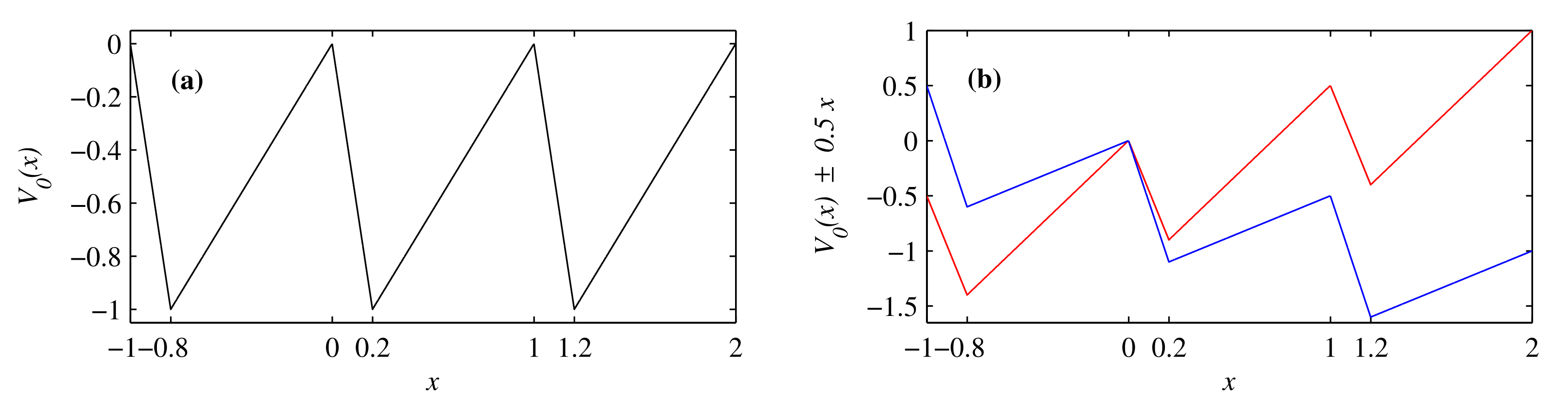
Here, $f=-{\partial }_{x}V$ is the force due to the potential $V(x,t)$. The potential $V(x,t)=V_0\left(x\right)+V_1(x,t)+V_2\left(x\right)$ contains the three parts. $V_0\left(x\right)=V_0(x+L)$ is a spatially periodic potential with the period L, $V_1\left(t\right)=-xG\left(t\right)$ is a time-dependent (rocking) potential given by a function $G\left(t\right)=G(t+T)$ that is periodic in time with period T, $V_2=-xF$ is a potential due to a constant force F. We note that T in this paper denotes a temporal periodicity of G and not temperature.

$\xi$ is assumed to have a zero mean $\langle \xi \rangle =0$ and the strength D with the following property

$$\langle \xi \left(t\right)\xi \left(t^{\prime }\right)\rangle =2D\delta (t-t^{\prime }),$$

(2)

where the angular brackets denote the ensemble average over $\xi$. We note that we are using the notation D for the fluctuation in heat bath (temperature) instead of T (the periodicity of the force $G\left(t\right)$).

The Fokker–Planck equation [39] for a time-dependent probability density function (PDF) $p(x,t)$ corresponding to Equations (1) and (2) is

$$\begin{array}{ccc}\hfill \frac{\partial }{\partial t}p(x,t)& =& -\frac{\partial J}{\partial x}=\frac{\partial }{\partial x}\left[\frac{\partial V}{\partial x}p(x,t)+D\frac{\partial }{\partial x}p(x,t)\right]\hfill \end{array}$$

(3)

where $V=V_0\left(x\right)-xG\left(t\right)-xF$; $J=-\left[\frac{\partial V}{\partial x}p(x,t)+D\frac{\partial }{\partial x}p(x,t)\right]=fp-D{\partial }_{x}p=(-{\partial }_x{V}_0+G\left(t\right)+F)p-D{\partial }_{x}p$ is the probability current.

Because of the spatial periodicity of $V_0\left(x\right)=V_0(x+L)$, we have $p(x,t)=p(x+L,t)$ and $J(x,t)=J(x+L,t)$. So, we normalise the PDF $p(x,t)$ over L as ${\int }_0^{L}dxp(x,t)=1$ at any time t. The ensemble average of a variable, say, $A(x,t)$, is then expressed in terms of the PDF of $A(x,t)$ as

$$\langle A\left(t\right)\rangle ={\int }_0^{L}dxA(x,t)p(x,t).$$

(4)

We use the double angular brackets to denote the average over the space and time, for instance

$$\langle \langle A\rangle \rangle =\frac{1}{T}{\int }_0^{T}dt{\int }_0^{L}dxA(x,t)p(x,t).$$

(5)

For the current J, Equations (4) and (5) translate to

$$\begin{array}{ccc}\hfill \langle J\rangle & =& \frac{1}{L}{\int }_0^{L}dxJ(x,t),\hfill \end{array}$$

(6)

$$\begin{array}{ccc}\hfill \langle \langle J\rangle \rangle & =& \frac{1}{LT}{\int }_0^{T}dt{\int }_0^{L}dxJ(x,t).\hfill \end{array}$$

(7)

2.1. Thermodynamic Relations

Thermodynamic laws concern the energy conservation and entropy relations and are provided in Appendix A and Appendix B for a general overdamped process. When $V=V_0\left(x\right)-xG\left(t\right)-xF$ in Equation (1) [$V_1(x,t)=-xG\left(t\right)$, $V_2\left(x\right)=-xF$], the energy conservation in Equation (A3) (with $\dot{W}={\dot{E}}_{in}$) can be expressed as

$$\begin{array}{ccc}\hfill \frac{d}{dt}\left(U_0+U_1+U_2\right)& =& \frac{d}{dt}\langle V\rangle \equiv {\dot{E}}_{in}-\dot{Q}.\hfill \end{array}$$

(8)

Here, $U_0={\int }_0^{L}dxp(x,t)V_0$, $U_1={\int }_0^{L}dxp(x,t)(-xG\left(t\right))$, and $U_2=-{\int }_0^{L}dxp(x,t)xF$, and ${\dot{E}}_{in}$ and $\dot{Q}$ are given by

$$\begin{array}{ccc}\hfill {\dot{E}}_{in}& =& {\int }_0^{L}dx\left({\partial }_{t}V\right)p=\langle {\partial }_t{V}_1\rangle =-{\int }_0^{L}dxx\dot{G}\left(t\right)p=-\langle x\dot{G}\rangle ,\hfill \end{array}$$

(9)

$$\begin{array}{ccc}\hfill \dot{Q}& =& -{\int }_0^{L}dxV\left({\partial }_{t}p\right)={\int }_0^{L}dxJf=\langle f\dot{x}\rangle =D{\dot{S}}_M.\hfill \end{array}$$

(10)

Here, ${\dot{E}}_{in}$ is the rate of energy input (e.g., by chemical agency, ATP, etc.) and $\dot{Q}$ the heat flow from the system to the environment. The rate at which a system does work against the external force is defined by

$${\dot{E}}_o=\frac{d{U}_2}{dt}=\frac{d}{dt}{\int }_0^{L}p(x,t)V_2=-F{\int }_0^{L}dx\left({\partial }_{t}p\right)x=F{\int }_0^{L}dx\left({\partial }_{x}J\right)x=-F{\int }_0^{L}dxJ.$$

(11)

Using Equations (9)–(11) in Equation (8) gives us

$$\begin{array}{ccc}\hfill \frac{d}{dt}\left(U_0+U_1\right)+\dot{Q}& =& {\dot{E}}_{in}-{\dot{E}}_o.\hfill \end{array}$$

(12)

The total energy input over one period T is given by the time-integral of Equation (9) as

$$\begin{array}{ccc}\hfill E_{in}& & =-{\int }_t^{t+T}d{t}_1{\int }_0^{L}dxx\dot{G}\left(t_1\right)p(x,t_1)={\int }_t^{t+T}d{t}_1{\int }_0^{L}dxxG\left(t_1\right)\dot{p}(x,t_1)\hfill \\ & & =-{\int }_t^{t+T}d{t}_1{\int }_0^{L}dxxG\left(t_1\right){\partial }_{x}J(x,t_1)={\int }_t^{t+T}d{t}_1{\int }_0^{L}dxG\left(t_1\right)J(x,t_1).\hfill \end{array}$$

(13)

Furthermore, over one period T, ${\int }_0^{T}d{t}_1\frac{d}{d{t}_1}(U_0\left(t_1\right)+U_1\left(t_1\right))=0$. Thus, Equation (12) is simplified as

$$Q=E_{in}-E_o.$$

(14)

Q in Equation (14) is related to the entropy flow $S_M$ from the system to the environment as $Q=D{S}_M$. It is also related to the entropy production $S_T=S+S_M\ge 0$ in Equation (A1) (see Appendix A for details), where $S=-{\int }_0^{L}dxp(x,t)lnp(x,t)$ is the differential entropy. Specifically, Equation (A2) reads

$$\begin{array}{c}\hfill {\dot{S}}_T=\frac{d{S}_T}{dt}={\int }_0^{L}dx\left(\frac{1}{Dp}{J}^2\right),{\dot{S}}_M=\frac{d{S}_M}{dt}={\int }_0^{L}dx\left(\frac{1}{D}Jf\right),\end{array}$$

(15)

where ${\dot{S}}_T$ and ${\dot{S}}_M$ denotes the entropy production rate and entropy flow rate, respectively. Equation (15) shows that ${\dot{S}}_T\ge 0$; ${\dot{S}}_T>0$ serves as a measure of irreversibility far from equilibrium. ${\dot{S}}_M$ is positive when the entropy flows from the system to the environment. Due to the periodicity of $p(x,t)=p(x,t+T)$, the total change over the cycle in the differential entropy $S={\int }_0^{T}d{t}_1\dot{S}\left(t_1\right)=0$. Thus, we have $S_T=S+S_M=S_M=Q/D\ge 0$ where

$$\begin{array}{c}\hfill S_T={\int }_0^{T}dt{\dot{S}}_T\left(t\right),S_M={\int }_0^{T}dt{\dot{S}}_M\left(t\right).\end{array}$$

(16)

2.2. Efficiency

Using the relations in Section 2.1, we have the instantaneous efficiency ($\eta$) and cumulative efficiency (${\eta }_c$) defined over one cycle as follows:

$$\begin{array}{ccc}\hfill \eta & =& \frac{{\dot{E}}_o}{{\dot{E}}_{in}},\hfill \end{array}$$

(17)

$$\begin{array}{ccc}\hfill {\eta }_c& =& \frac{E_o}{E_{in}}=1-\frac{Q}{E_{in}}=1-\frac{D{S}_T}{E_{in}}.\hfill \end{array}$$

(18)

Equation (18) shows explicitly that the non-zero entropy production $S_T>0$ or heat flow Q reduces the efficiency.

To take into account the viscous work ${\dot{E}}_s=\gamma {\langle \dot{x}\rangle }^2=\gamma {\left[\int dxJ\right]}^2$ ($\gamma =1$ for Equation (1)), Equations (17) and (18) were generalised to include the Stokes efficiency [40,41] as follows

$$\begin{array}{ccc}\hfill \eta & =& \frac{{\dot{E}}_o+\dot{E_s}}{{\dot{E}}_{in}}=\frac{\dot{E_s}}{{\dot{E}}_{in}},\hfill \end{array}$$

(19)

$$\begin{array}{ccc}\hfill {\eta }_c& =& \frac{E_s}{E_{in}},\hfill \end{array}$$

(20)

where $E_s={\int }_t^{t+T}d{t}_1{\dot{E}}_s\left(t_1\right)$.

We note that even when there is no external force $F=0$, the system can generate a non-zero current $\langle \langle J\rangle \rangle >0$. A stopping force $F_s<0$ is the force that is required to make the current zero $\langle \langle J\rangle \rangle =0$ above/below which the sign of the current changes ($\langle \langle J\rangle \rangle >0$ for $F>F_s$ and $\langle \langle J\rangle \rangle <0$ for $F<F_s$). To separate the additional effect of $F\ne 0$, we will focus on $F=0$ in Section 3, Section 4 and Section 5. Moreover, since in our problem (e.g., for a sinusoidal $G\left(t\right)$) ${\dot{E}}_{in}$ can take zero value at certain time with a singular $\eta$, we will calculate ${\eta }_c$ in Equation (20) in Section 3, Section 4 and Section 5.

2.3. Information Rate and Length

Information rate $\mathrm{\Gamma }$ and length $\mathcal{L}$ are the information geometric measures that quantify how information unfolds in time-varying stochastic processes [18,27,28,29,30,31,32,33,34,35,36,37,38]. In a nutshell, $\mathrm{\Gamma }$ is proportional to the square root of infinitesimal (symmetric) relative entropy (Kullback–Leibler divergence) while $\mathcal{L}$ measures the total change in the information along its evolution path. For example, for a PDF of one variable x evolving in time t,

$$\begin{array}{ccc}& & {\mathrm{\Gamma }}^2\left(t\right)=\int dxp(x,t){({\partial }_{t}lnp(x,t))}^2=4\int dx{\left({\partial }_{t}q\left(t\right)\right)}^2,\hfill \end{array}$$

(21)

$$\begin{array}{ccc}& & \mathcal{L}\left(t\right)={\int }_0^{t}d{t}_1\mathrm{\Gamma }\left(t_1\right).\hfill \end{array}$$

(22)

We note that ${\mathrm{\Gamma }}^2$ in terms of $q=\sqrt{p}$ is well defined for $p=0$. When the parameters of $p(x,t)$ are known as ${\lambda }_i$’s ($i=1,2,\dots$), ${\mathrm{\Gamma }}^2$ can be expressed in terms of the metric tensor $g^{ij}=\int dxp(x,t)({\partial }_{{\lambda }_i}lnp(x,t))({\partial }_{{\lambda }_j}lnp(x,t))$ as ${\mathrm{\Gamma }}^2={\sum }_{i,j}\left({\partial }_t{\lambda }_i\right)g^{ij}\left({\partial }_t{\lambda }_j\right)$.

${\mathrm{\Gamma }}^{-1}$ has the dimensions of time and is linked to the smallest timescale of fluctuations [38]. As a non-decreasing function of time, $\mathcal{L}\left(t\right)$ is a dimensionless, path-dependent distance measuring the deviation from the initial state in terms of the total number of statistically different states that a system passes through. For a Gaussian PDF with a constant variance, $\Delta \mathcal{L}=1$ when $p(x,t)$ moves from $p(x,0)$ by one standard deviation since the latter provides the uncertainty in measuring the PDF position. Even when $p(x,0)=p(x,T)$, $\mathrm{\Gamma }\left(t\right)$ is sensitive to temporal changes at $0<t<T$ and take different values depending on the path. $\mathrm{\Gamma }\left(t\right)$ and $\mathcal{L}\left(t\right)$ are invariant under (time-independent) change of variables (unlike entropy), enabling us to compare the evolution of different variables.

We measure the change in information associated with the dynamics of a Brownian ratchet by calculating

$$\mathcal{L}={\int }_0^{T}d{t}_1\mathrm{\Gamma }\left(t_1\right),$$

(23)

over the time interval of one period. Equation (23) represents the total number of different statistical states that a ratchet passes through in one period.

3. Numerical Models and Methods

3.1. Potential $V_0\left(x\right)$ and Rocking Force $G\left(t\right)$

As noted in Section 1, we consider a sawtooth potential $V_0\left(x\right)$, as shown in the first panel of Figure 1. Note first how $V_0\left(x\right)$ is periodic in x, with period 1. Any other period L could always be rescaled to 1 by introducing a new variable $\tilde{x}=x/L$, so there is no loss of generality in only considering $L=1$. $V_0$ then has maxima at $x=0mod\left(1\right)$ and minima at $x=0.2mod\left(1\right)$. The particular value $x=0.2$ as the location of the minimum is not critical, as long as it is not at 0.5, which would yield a potential that was symmetric under $x\to -x$. In contrast, this potential $V_0\left(x\right)$ is clearly asymmetric under $x\to -x$, and this asymmetry underlies the entire rocking ratchet problem.

In particular, consider what happens if $V_0\left(x\right)$ is rocked back and forth, by the addition of the term $V_1\left(t\right)=-xG\left(t\right)$. Suppose that the maximum positive and negative amplitudes of $G\left(t\right)$ are $\pm A$, for some constant A. The second panel in Figure 1 shows the results for $A=0.5$: the original $V_0\left(x\right)$ is simply rocked back and forth. Now, consider what would happen to any particles situated in the $V_0$ potential wells. For this particular rocking amplitude of $0.5$, nothing would happen yet (at least in the absence of any noise), because the local minima always remain local minima throughout the entire rocking process. However, by considering the slopes of $V_0\left(x\right)$ on its two segments, that is, $-5$ on $x\in [0,0.2]$ and $1.25$ on $x\in [0.2,1]$, we see that if A had been chosen in the range $1.25<A<5$, any particles in the potential wells would always spill over to the right at that point in the rocking cycle but would never spill back to the left even at the opposite point in the cycle. This is the essence of the ratchet mechanism; the original asymmetry in $V_0\left(x\right)$ causes this spill-over effect to be uni-directional, resulting in a directed particle current. The interesting dynamics about this problem are then all about what happens in the presence of noise, how do the resulting current and other diagnostics vary with the amplitude and period of the rocking, etc.

There are various possible choices for the time-dependence $G\left(t\right)$ of the rocking. One simple choice is sinusoidal,

$$\begin{array}{ccc}\hfill G\left(t\right)& =& Asin\left(\omega t\right),\hfill \end{array}$$

(24)

where $\omega =2\pi /T$ relates the frequency $\omega$ to the period T. Another choice is a square wave, with

$$\begin{array}{ccc}\hfill G\left(t\right)& =& \{\begin{array}{ccc}\phantom{-}A& 0\le t<T/2& mod\left(T\right),\\ -A& T/2\le t<T& mod\left(T\right).\end{array}\hfill \end{array}$$

(25)

A third choice is a sawtooth wave, with

$$\begin{array}{ccc}\hfill G\left(t\right)& =& A(1-2t/T)0\le t<Tmod\left(T\right),\hfill \end{array}$$

(26)

consisting of a linear variation from A at $t=0$ to $-A$ at $t=T$, followed by a discontinuous jump back to A for the next period, etc.

Note also that positive versus negative A in Equation (26) are not equivalent—unlike in Equation (24) or (25), where changing the sign of A merely shifts $G\left(t\right)$ by half a period in time. In contrast, in Equation (26) positive and negative A are different, in the following sense: taking A positive starts with the upward sloping potential in Figure 1b, gradually tilts that to the downward sloping potential, then discontinuously jumps back to the upward sloping potential, etc. Because the original $V_0\left(x\right)$ already introduced the $\pm x$ asymmetry, this is different from what a negative A would do, namely to have the gradual tilting going from downward to upward sloping.

Since we prefer to always think of the amplitudes A as being positive though, we modify our definition of the sawtooth wave to be

$$\begin{array}{ccc}\hfill G_{\pm }\left(t\right)& =& \pm A(1-2t/T)0\le t<Tmod\left(T\right),\hfill \end{array}$$

(27)

so that now we have two different sawtooth waves, but each one separately can be restricted to considering only $A>0$, just as for the sinusoidal and square wave choices. We will see then that the two choices $G_{\pm }$ yield results that are very similar in some diagnostic quantities but different in others.

3.2. Numerical Methods

To numerically solve the Fokker–Planck Equation (3), with a spatially periodic potential, we use the following

$$p(x,t)=a_0\left(t\right)+\sum _{k=1}^K\left(a_k\left(t\right)cos\left(2\pi kx\right)+b_k\left(t\right)sin\left(2\pi kx\right)\right).$$

(28)

See also [42] for the theory underlying Fourier series in numerical analysis. The coefficients $a_k$ and $b_k$ are then time-stepped using second-order Runge–Kutta [43]. The term $\frac{\partial }{\partial x}\left(\frac{\partial V}{\partial x}p\right)$ is separated out into the relevant Fourier components using a fast Fourier transform. Since our chosen potential $V_0\left(x\right)$ has discontinuous derivatives, special attention is required to ensure that results are adequately resolved.

Resolutions in the range $K=2^{12}-2^{20}$ were used and time-steps in the range ${10}^{-4}-{10}^{-6}$. One very basic test of the numerical implementation is simply to monitor the coefficient $a_0$: this is time-stepped along with the others but must, in fact, remain constant if the total probability $\int pdx=a_0$ is to remain constant. It was found that if the initial condition is set to have $a_0=1$, then this was indeed preserved throughout the subsequent evolution. Note that there are also other numerical methods of solving Fokker–Planck equations that are very different from the direct time-stepping implemented here, instead using a variety of neural network approaches (e.g., [44,45,46]).

Since we are not interested in initial transients, but only in the final solutions $p(x,t)$ that are periodic in both x (with period 1) and t (with period T), we start with the very simple initial condition $a_0=1$ and all other Fourier coefficients set to zero, and integrate for however many periods T are required to settle in to a solution that is periodic in time. For some parameter choices this happened after just a few periods, but for other parameter choices many dozens of periods were required, significantly increasing the total computational effort.

As noted above, throughout this entire evolution the solutions always maintained $a_0=1$, but this is not a sufficiently stringent check to convince ourselves that the numerics are adequately dealing with the rather challenging potential $V_0\left(x\right)$. To see how the code is coping with this, Figure 2 shows some sample results for the sinusoidal choice Equation (24) with $A=6$ and two noise levels D as indicated in the figure. Note that, in particular, according to our arguments above, this A value is sufficiently large that spill-over should occur in both directions at different points in the rocking cycle. Sure enough, at different times the solutions are concentrated at locations far away from the $x=0.2$ potential well of just $V_0\left(x\right)$ alone.

If we focus on the PDFs at $t=0mod\left(T\right)$ though, they do indeed form a peak around $x=0.2$, with the width also becoming narrower as D is decreased. The first panel in Figure 3 examines this in more detail, showing how the width scales as D and the height as $1/D$. Note also how the solutions appear to be forming true cusps at $x=0.2$, with p continuous but ${\partial }_{x}p$ discontinuous at $x=0.2$. This is exactly what one would expect, based on the discontinuity in $\frac{d}{dx}{V}_0\left(x\right)$. The second panel in Figure 3 shows the corresponding Fourier power spectra $a_k^2+b_k^2$. Note how they are flat up to a certain k, and then start dropping off. Decreasing D by an order of magnitude increases the transition value of k by an order of magnitude, corresponding to the width scaling as D. Finally, once the wave-numbers k are sufficiently large to be well in the drop-off regime, the power scaling is as $k^{-4}$. From the general theory of Fourier series, this is exactly what one expects from a function that is continuous but with discontinuities in its first derivative. We see therefore that this potential $V_0\left(x\right)$ is challenging, especially at very small D, but that if one is prepared to set the Fourier series resolution K sufficiently high, any arbitrarily small D can still be achieved and yields a well-resolved power spectrum.

In the following section, we will present systematic scans over a range of A values for D as small as ${10}^{-3}$, which is already small enough for clear trends to emerge. We will focus in particular on the diagnostic quantities current (Equation (7)), efficiency (Equation (20)), $\mathcal{L}$ (Equation (23)) and $S_T$ (Equation (16)) integrated over the period T and then mapped out as functions of A, as well as some representative cases of current (Equation (6)), $\mathrm{\Gamma }$ (Equation (21)), $\dot{S}$ (Equation (A1)) and ${\dot{S}}_T$ (Equation (15)) as functions of time over a period.

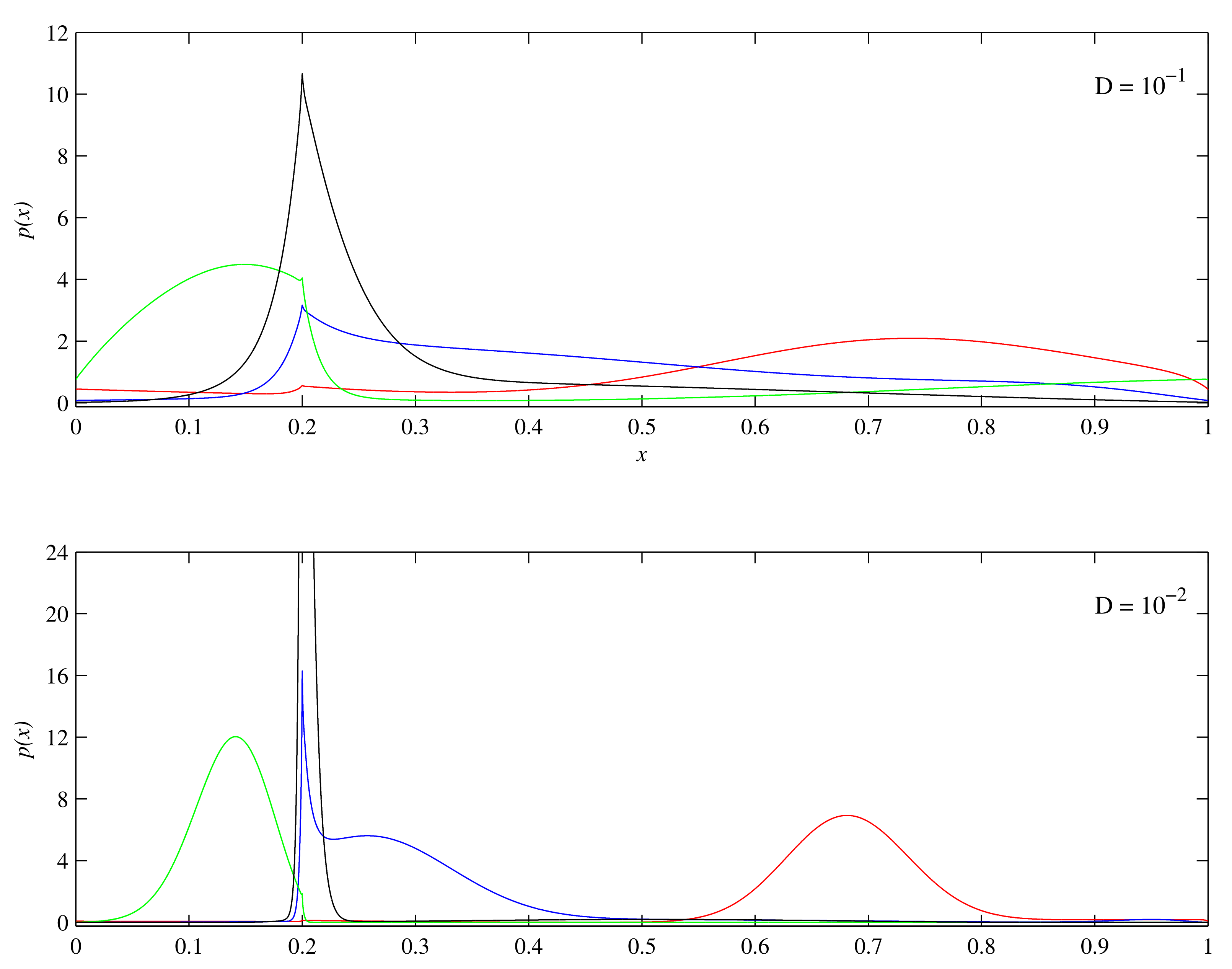
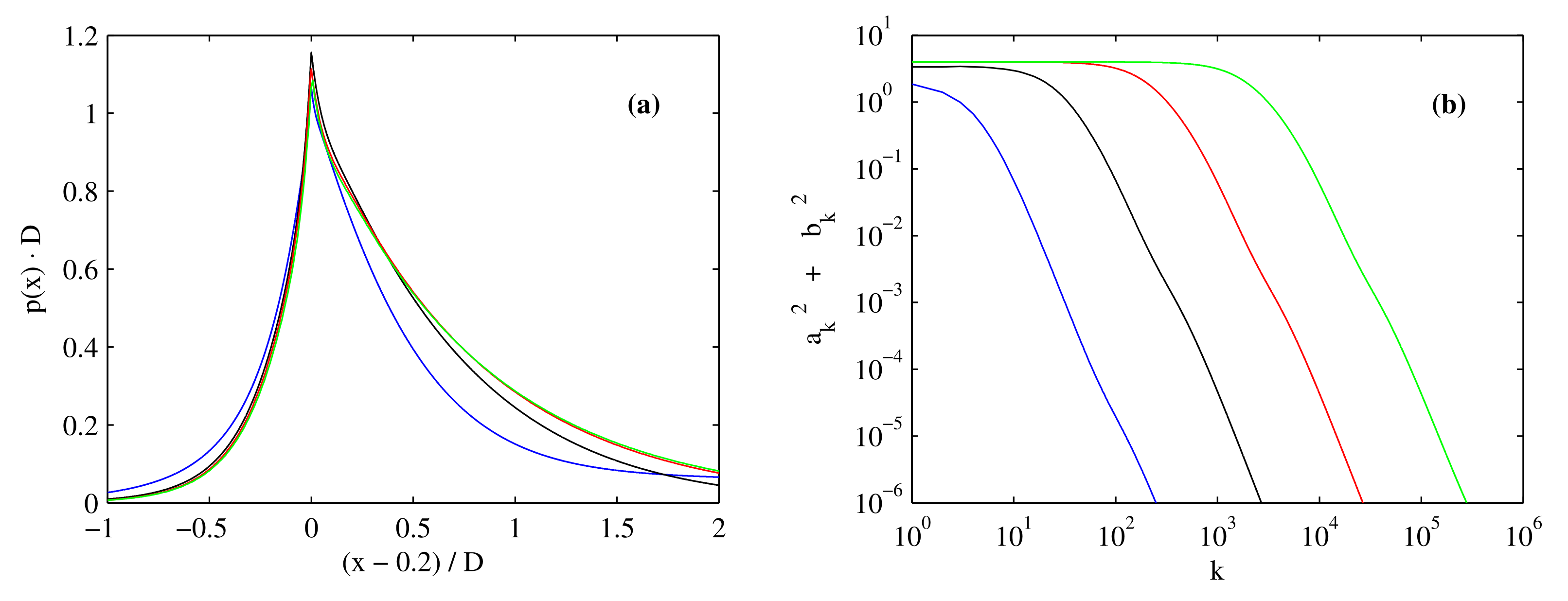
4. Results for $\mathit{G}\left(\mathit{t}\right)=\mathit{A}sin\left(\mathit{\omega }\mathit{t}\right)$

We start with the sinusoidal rocking Equation (24). We investigated a variety of periods T, ultimately focusing on the four values $T=0.4$, $0.7$, 1 and 2 to consider in detail. For each of these, we scanned over the range $A\in [0,20]$, for the three noise values $D={10}^{-1}$, ${10}^{-2}$ and ${10}^{-3}$.

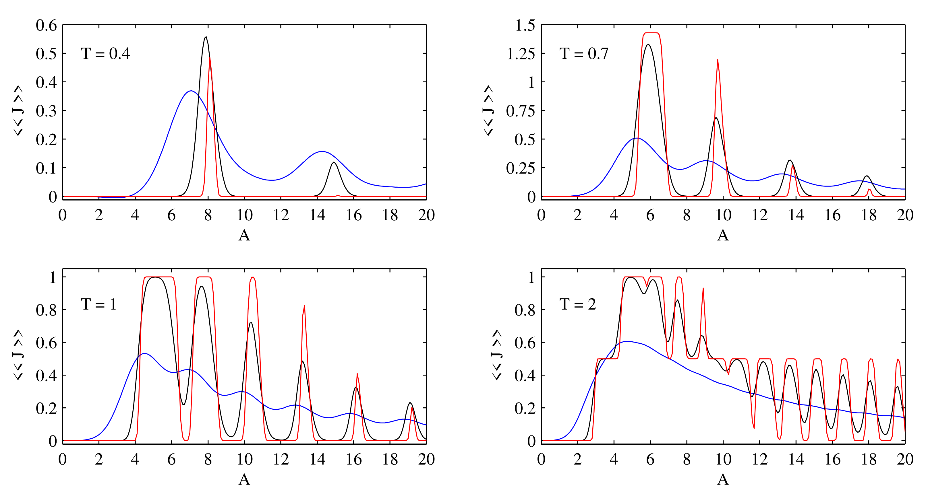
Figure 4 shows the current $\langle \langle J\rangle \rangle$ from Equation (7). One feature that immediately stands out is how $\langle \langle J\rangle \rangle$ tends to zero if A is too small, consistent with our discussion above regarding the dynamics of the ratchet mechanism, and why there is a non-zero current at all. It is also noticeable that $\langle \langle J\rangle \rangle$ is much less for $T=0.4$ than for the larger values. This is also as one might expect: if the system is rocked back and forth too rapidly, there simply is not enough time for much spill-over to occur, even if A is large enough that it otherwise would. For T even smaller than 0.4, the current also becomes even smaller.

Regarding the variation with D, we note how the various peaks become increasingly sharp and distinct as D is reduced. The limit $D\to 0$ would consist of a set of peaks that vary discontinuously with A, being either zero or $1/nT$, for $n=1,2,\dots$ (e.g., see [47]). To understand such a complicated pattern, and why the current does not vary monotonically with A, we recall that once $A>5$ for our particular $V_0$ here, the spill-over can also go to the left, the opposite of the ‘desired’ direction. When $\langle \langle J\rangle \rangle$ abruptly drops to zero are then values of A where this negative spill-over occurred, whereas $\langle \langle J\rangle \rangle$ jumps back to some non-zero value for those values of A where the positive spill-over extends one further well of $V_0$ than before.

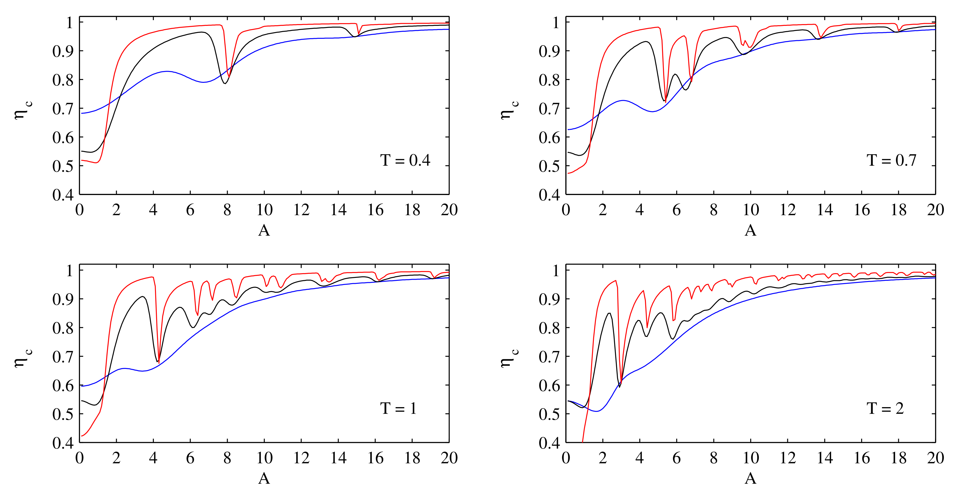
Figure 5 shows the Stokes efficiency ${\eta }_c$ from Equation (20). If A is too small it is relatively small, but for larger A it can approach 1, even for $T=0.4$ where the current was small. As with the current, there are various up-and-down jumps that become sharper and more distinct for smaller D. Comparing Figure 4 and Figure 5, one can already see that the jumps in $\langle \langle J\rangle \rangle$ and ${\eta }_c$ occur at similar values of A; we will consider this phase relationship between these quantities in more detail below (Figure 8).

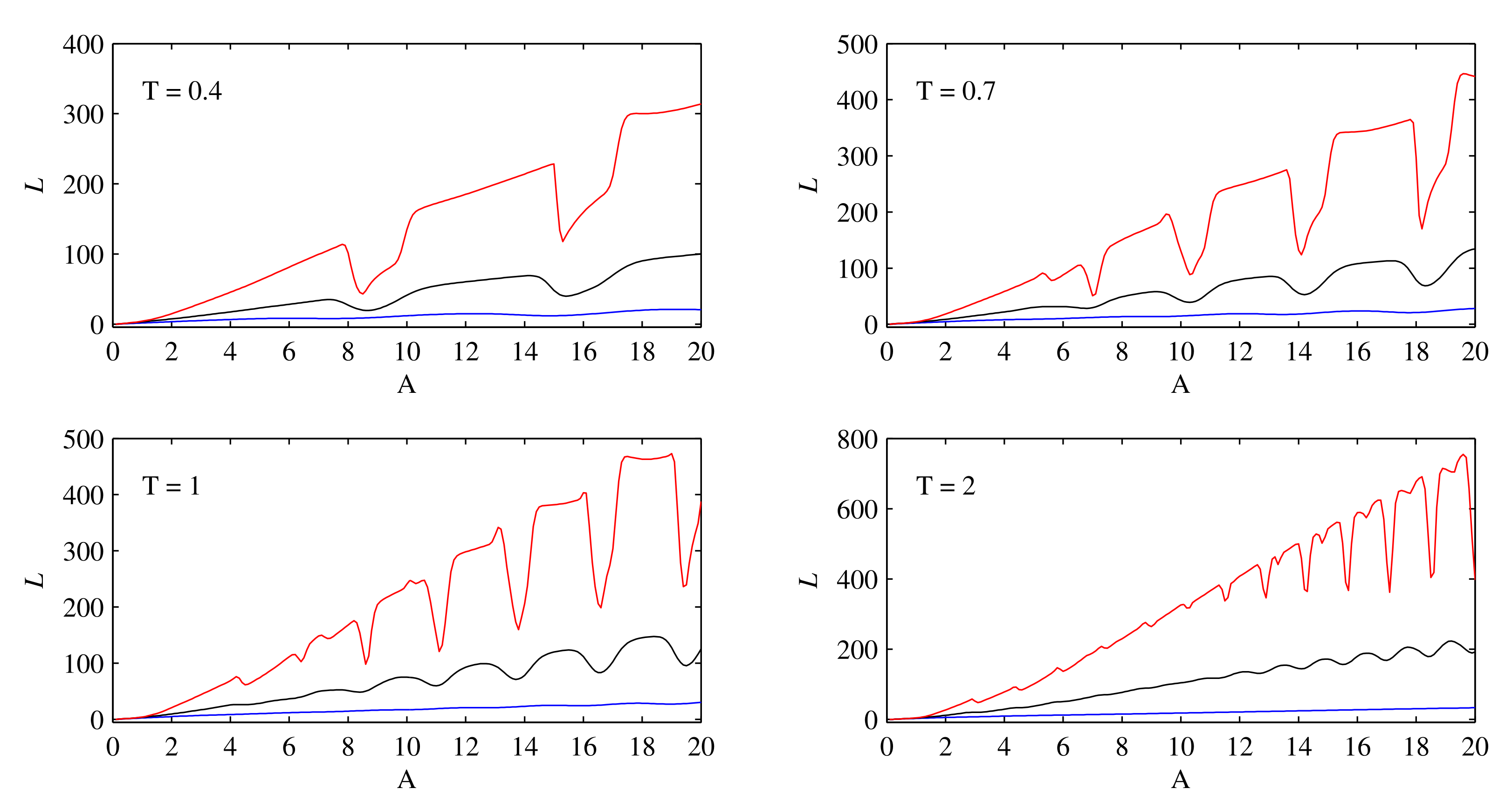
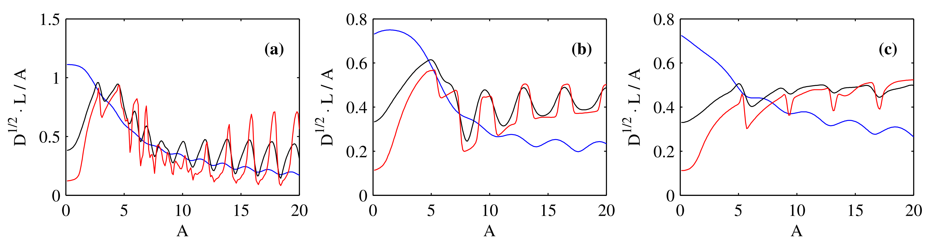
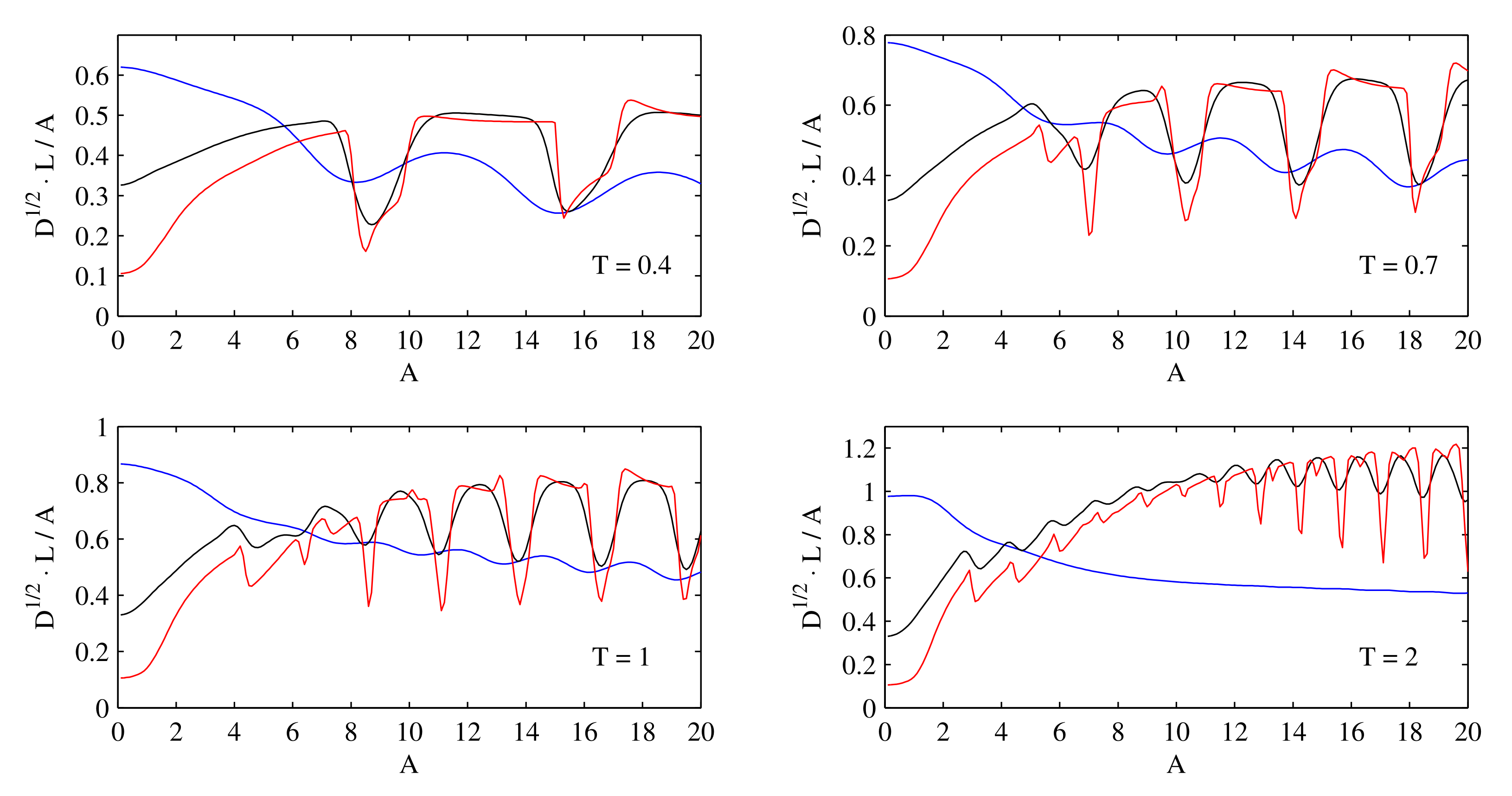
Figure 6 shows the information length $\mathcal{L}$ from Equation (23). The two features that immediately stand out are that $\mathcal{L}$ generally increases with increasing A, and decreasing D. This suggests to collapse the results by instead plotting $\mathcal{L}·D^{1/2}/A$. As shown in Figure 7, this does indeed remove the overall increase with A, allowing one to focus more on the jumps that are similar to those seen before in the current and efficiency. Figure 7 also suggests that in the $D\to 0$ limit, this combination might become independent of D, including the details of the various jumps. However, D would have to be reduced quite a bit further to fully clarify this question. The overall trend though that $\mathcal{L}$ is broadly proportional to $D^{-1/2}$ is very likely robust. Roughly speaking, this is (i) because $\mathcal{L}$ is a dimensionless distance that measures the change in the mean location of a PDF (mean value) with respect to the measurement error given by the standard deviation (width of a PDF) as long as the mean (A) is not too small compared with the standard deviation and (ii) the change in the mean and standard deviation increase with A and $D^{1/2}$, respectively.

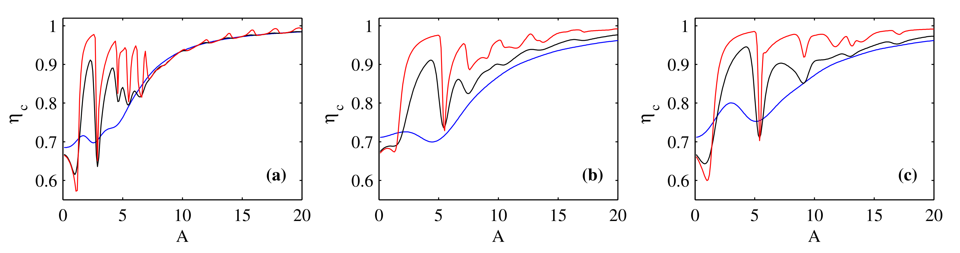
The three quantities presented so far, $\langle \langle J\rangle \rangle$, ${\eta }_c$ and $\mathcal{L}{D}^{1/2}/A$, all exhibit similar up and down jumps as A is increased. To clarify the phase relationships between these quantities, Figure 8 super-imposes the three, for the $D={10}^{-3}$ case where the jumps become clearest. The range in A is also restricted to $A\in [3,15]$ to focus on the first few jumps. Only $T=0.7$ and 1 are shown here, but 0.4 and 2 exhibited similar behaviour. In particular, we see how the jumps in all three quantities are indeed very closely correlated, with maxima or minima in ${\eta }_c$ and $\mathcal{L}{D}^{1/2}/A$ tending to line up with those A values where $\langle \langle J\rangle \rangle$ is changing most rapidly. This suggests that our (normalised) information geometric diagnostics $\mathcal{L}{D}^{1/2}/A$ approximates the Stokes efficiency better than the current. We however notice that the phase relations seem to be less clear for larger $A\ge 10$.

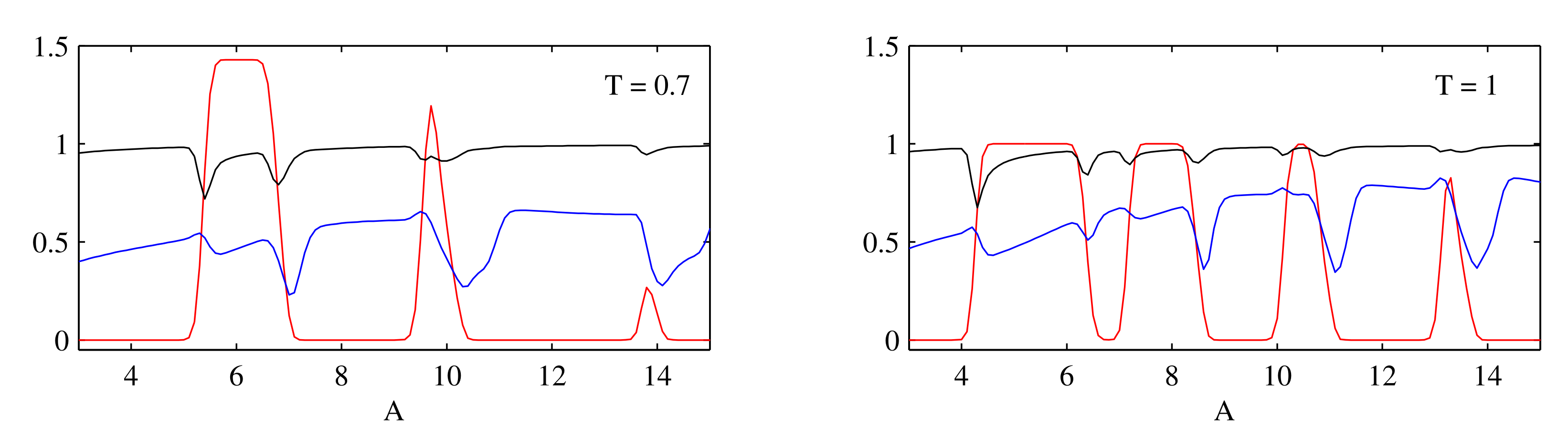
Based on Figure 8, the particular values $A=6,7,8$ for $T=0.7$ represent one of the transitions from $\langle \langle J\rangle \rangle$ being large at $A=6$ to essentially zero at $A=8$, and correspondingly $A=7$ is a minimum for $\mathcal{L}$. The first two panels in Figure 9 then show the variation in time of the quantities $\langle J\rangle$ and $\mathrm{\Gamma }$. Note how $\langle J\rangle$ is positive for almost the entire cycle for $A=6$, which is why $\langle \langle J\rangle \rangle$ is so large at this A. For $A=7$ and 8, $\langle J\rangle$ is if anything slightly greater for the first half of the cycle, but for the second half it is strongly negative. This is precisely the point noted above, that for sufficiently large A the spill-over can also go in the ‘wrong’ direction, reducing the average current $\langle \langle J\rangle \rangle$ to essentially zero at $A=8$.

In comparison, $\mathrm{\Gamma }$ measures the rate at which the change in a PDF occurs, taking a large value when a PDF changes rapidly. Thus, a spill-over regardless of its direction can cause a sudden change in a PDF shape. This is seen in Figure 9 where $\mathrm{\Gamma }$ tends to be large at points in the cycle where the absolute value of $\langle J\rangle$ is also large. That is, $\mathrm{\Gamma }$ is insensitive to the sign of any spill-over, but it does measure that spill-over is occurring. Furthermore, the first peak of $\langle J\rangle$ occurs at different times $t\sim 0.2,0.25$ for $A=6,7,8$, while the peak of $\mathrm{\Gamma }$ occurs at a similar time $t\sim 0.12$, earlier than that of $\langle J\rangle$. This suggests that $\mathrm{\Gamma }$ detects a rapid change in a PDF prior to the appearance of $\langle J\rangle$ peak.

Panels (c,d) in Figure 9 show the variation in time of the quantities $\dot{S}$ and ${\dot{S}}_T=\dot{S}+{\dot{S}}_M$. A few points to note here are: First, $\dot{S}$ can be both positive and negative, see Equation (A1), and indeed integrates to zero due to the temporal periodicity $S\left(t\right)=S(t+T)$, as noted in Section 2.2. In contrast, ${\dot{S}}_T$ is strictly non-negative, as it must be according to Equations (15) and (16). Next, we can note that a typical magnitude of $\dot{S}$ is roughly 50 times smaller than a typical magnitude of ${\dot{S}}_T$, $O\left(100\right)$ versus $O(50,000)$. Finally, if we compare $\dot{S}$ with $\langle J\rangle$ in the panel directly above it, we notice that the jumps in $\dot{S}$ almost invariably line up with certain features in $\langle J\rangle$, for each of the three values $A=6,7,8$. It seems therefore that $\dot{S}$ is also sensitive to the spill-over dynamics that cause variations in $\langle J\rangle$. This is because the spill-over inevitably causes the change in a PDF such as broadening or narrowing of a PDF width and thus entropy.

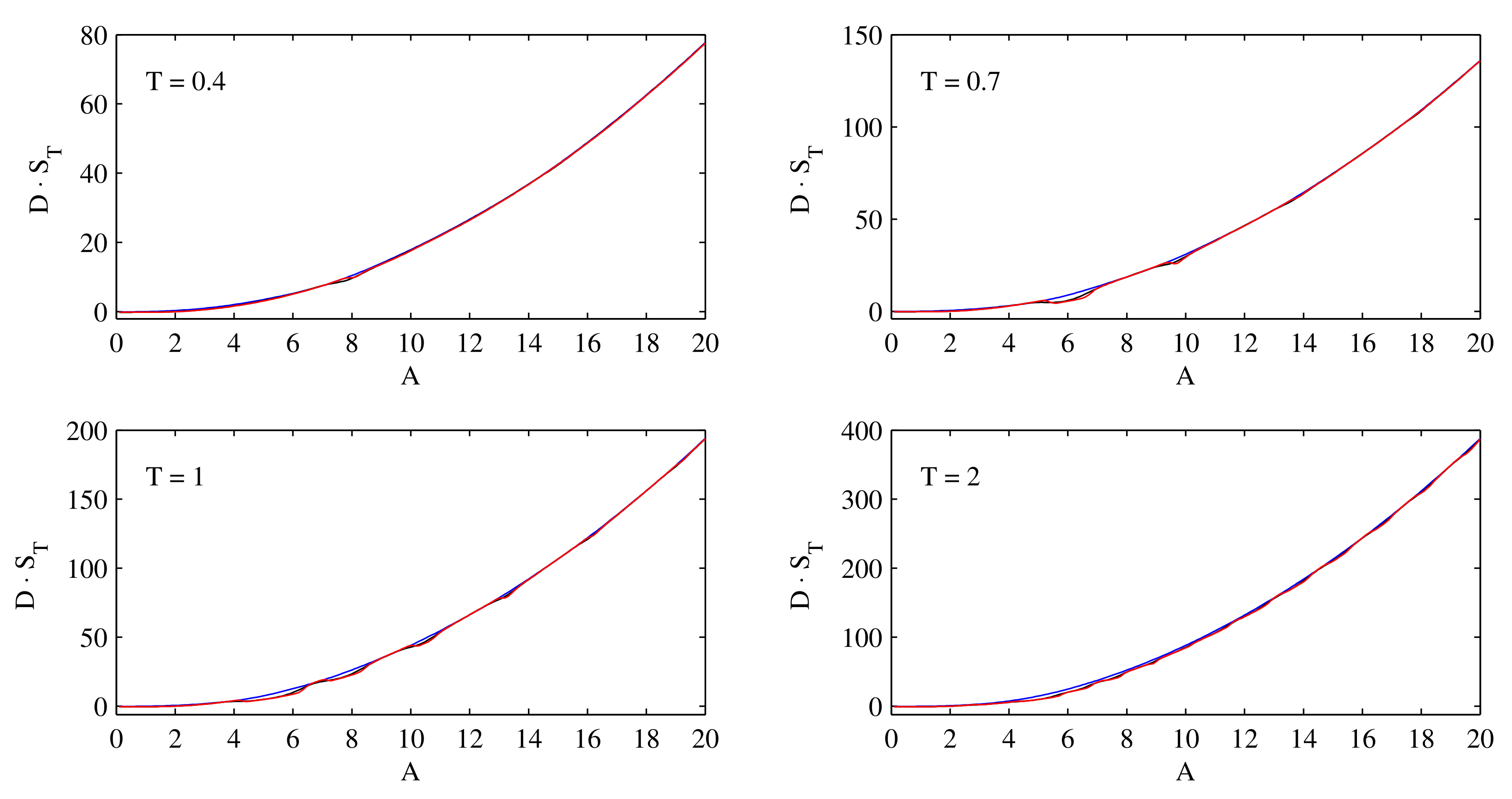
Figure 10 shows the period-integrated quantity $D·S_T=D·S_M$, for the same parameter values as before in Figure 4, Figure 5, Figure 6 and Figure 7. There are again three curves in each panel, with the same colour-coding as before, but we see that the three curves almost completely overlap virtually everywhere. That is, the scaling $S_T\sim D^{-1}$ holds so accurately that $D{S}_T$ becomes almost completely identical for the three different D values. The other point to note is how the curves in all four panels are following parabolic profiles for all but the very smallest values of A. That is, once $A>5$ or so, $S_T\sim A^2$ becomes an almost exact fit.

5. Results for Square and Sawtooth $\mathit{G}\left(\mathit{t}\right)$

Similar scans were performed for the square wave Equation (25) and sawtooth waves Equation (27). We will only present $T=1$ here; other values were also considered and exhibited similar trends. Figure 11 again shows the current $\langle \langle J\rangle \rangle$ as a function of A, for the same three D values as before. We note how the maximum value of $\langle \langle J\rangle \rangle$ for the square wave is twice what it was for the sinusoidal $G\left(t\right)$ and also for the sawtooth waves. This simply reflects the fact that the square wave $G\left(t\right)=\pm A$ has twice the rms value as the sinusoidal $G\left(t\right)$. Another interesting point is that $\langle \langle J\rangle \rangle$ for the square wave does not seem to drop back to zero between the various peaks, unlike for the sinusoidal or sawtooth waves. Finally, note how the two sawtooth waves $G_{\pm }$ yield virtually identical results for this particular diagnostic quantity $\langle \langle J\rangle \rangle$.

Figure 12 shows the Stokes efficiency ${\eta }_c$. The results are again broadly similar to the sinusoidal results in Figure 5, with efficiencies approaching one in all cases. Again, just as before the particularly small currents for the sinusoidal $G\left(t\right)$ with $T=0.4$ had no particular effect on the efficiency, here also the particularly large currents for the square wave have no discernible effect on its efficiency. Another point to note here is that the results for the two sawtooth waves are still similar, but noticeably different, unlike in Figure 11 where the currents were virtually identical.

Finally, for the information length $\mathcal{L}$, we dispense with the plots of $\mathcal{L}$ itself and proceed directly to plots of $\mathcal{L}{D}^{1/2}/A$, as shown in Figure 13. The overall pattern is again similar to what it was for the sinusoidal $G\left(t\right)$. In particular, there is again at least the suggestion that this combination might be tending to a limit independent of D, but considerably smaller values would be required to confirm this. The last point to note is that now the results for the two sawtooth waves $G_{\pm }$ are significantly different, more even than previously for the Stokes efficiency. Information length is evidently a very delicate diagnostic quantity that picks out differences in PDFs that other diagnostics are far less sensitive to.

6. Conclusions

We investigated exact time-dependent solutions of a Brownian motor under different conditions to elucidate the role of symmetry-breaking and information geometry. Specifically, we utilised an asymmetric sawtooth periodic potential and three different types of periodic forcing $G\left(t\right)$ given by sinusoidal, square and sawtooth waves with period T and amplitude A. For each $G\left(t\right)$, we calculated exact time-dependent probability density functions (PDFs) by numerically solving the Fokker–Planck equation [39] under different conditions by varying T, A and the strength of the stochastic noise D in an unprecedentedly wide range. We showed that a non-differentiable potential led to a non-differentiable PDF and ensured that our solutions were well resolved by including a sufficiently large number of Fourier modes. From our time-dependent PDF, we performed a systematic investigation of comparing mean current, Stokes efficiency, entropy production and the path-dependent information geometric measures (information rate and information length). Interestingly, regardless of different forms of $G\left(t\right)$, we found overall similar behaviours. This highlights the essential role of symmetry-breaking and robustness of the results that are less sensitive to the detailed temporal evolution of a motor (driven by different forcings $G\left(t\right)$).

In particular, current, Stokes efficiency and the information rate normalised by A and D exhibit one or multiple local maxima and minima as A increases. However, the dependence of current and Stokes efficiency on A can be quite different, while the information rate normalised by A and D tends to resemble that of the Stokes efficiency. In comparison, the irreversibility measured by a normalised entropy production is independent of A. The results thus suggest that the entropy production is not a good measure of a motor efficiency. Instead, our information geometry provides a useful proxy of the Stokes efficiency. Whether this result holds in general when there is a non-zero constant external force F in our model Equation (1) will be investigated in future. Future work will also address different types of Brownian motors such as the (two-state) flashing ratchet [48] driven by the dichotomous noise in addition to a short-correlated noise or Levy-type noise. It will also be of interest to compare our path-dependent information geometric theory with other measures of irreversibility such as the Komogorov eigenvalue or non-equilibrium Lyapunov function [49].