
Copula-Based Estimation Methods for a Common Mean Vector for Bivariate Meta-Analyses


Abstract
:1. Introduction
2. Background
2.1. Bivariate Meta-Analysis
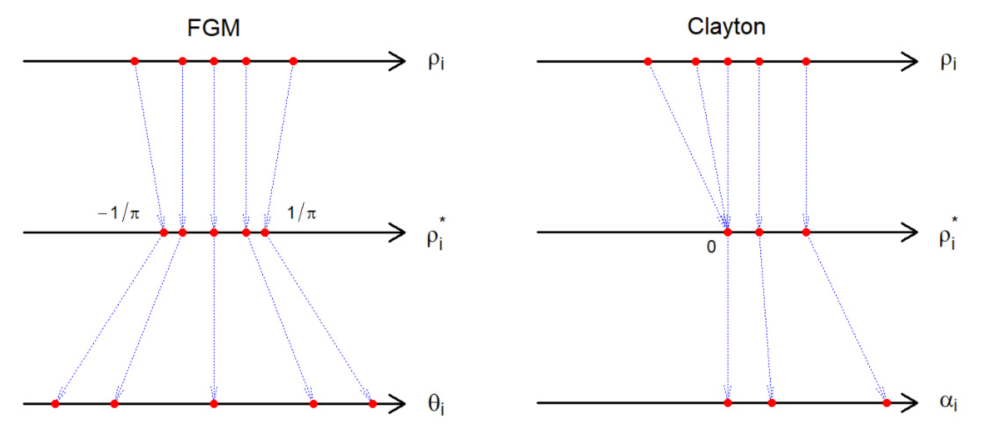
2.2. Copulas
3. Proposed Methods
3.1. General Copula Model for the Common Mean
3.2. Statistical Inference Methods
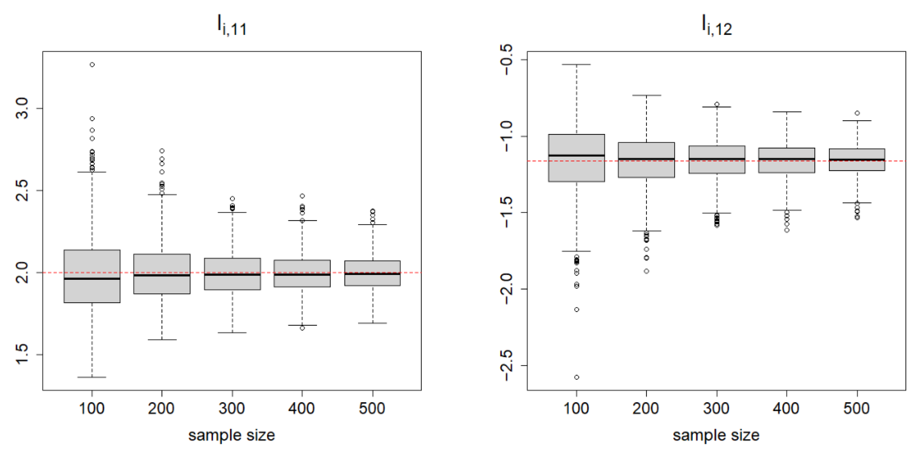
3.3. Information Matrix
4. Asymptotic Theory
- (a)
- Existence and consistency: With probability tending to one, there exists the MLEsuch that, as;
- (b)
- Asymptotic normality:, as.
5. SE and Confidence Sets
6. R Package
 |
 |
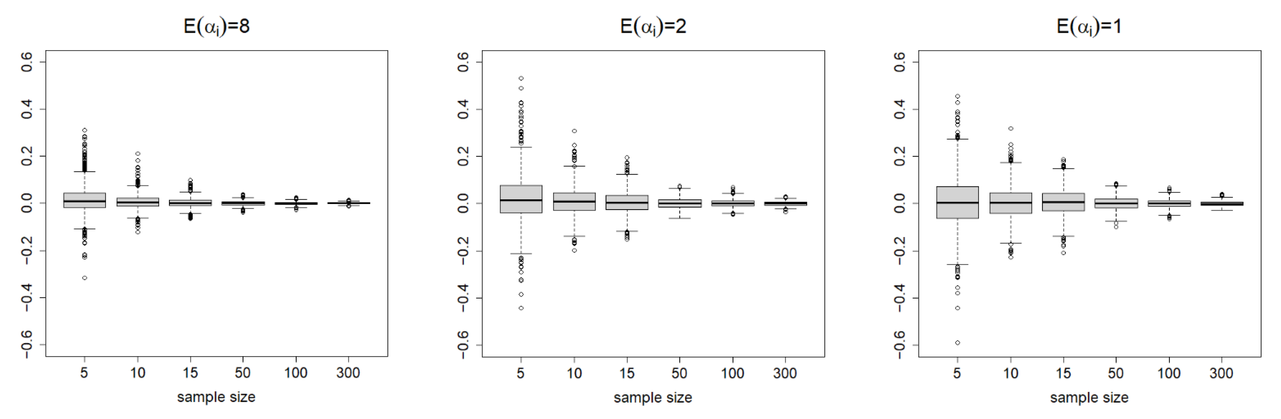
7. Simulation Studies
8. Data Analysis
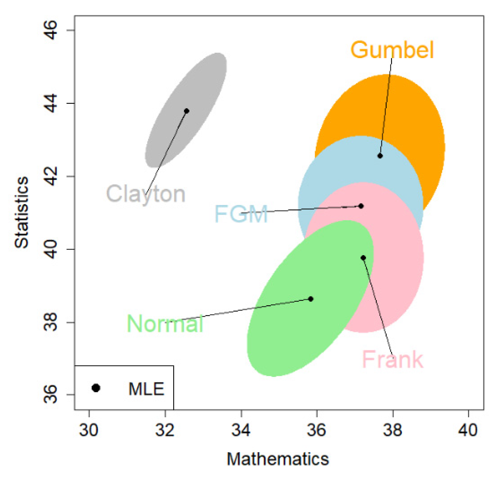
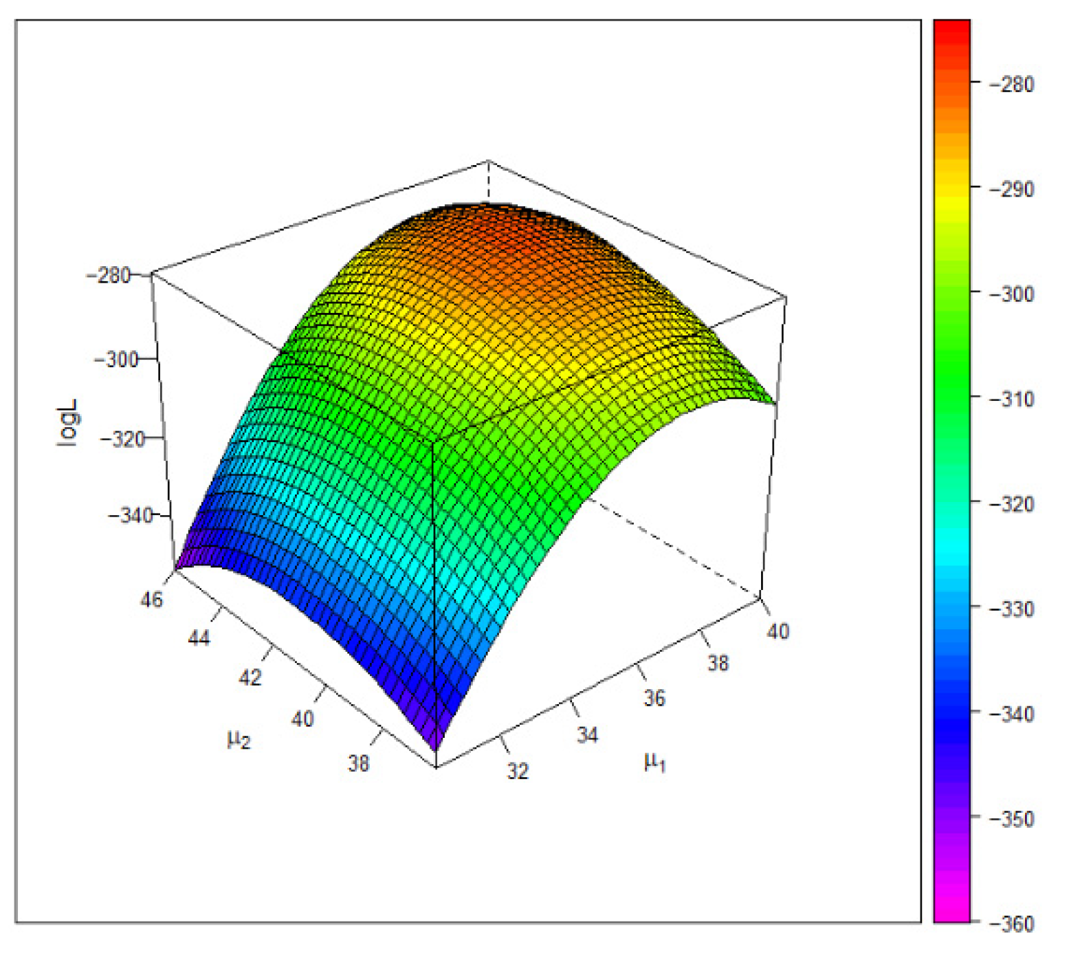
8.1. The Entrance Exam Data
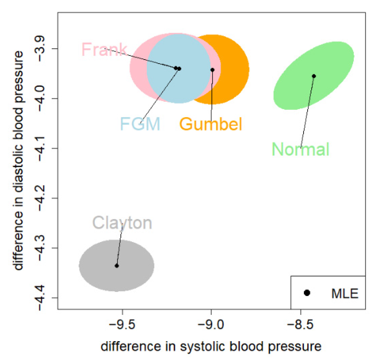
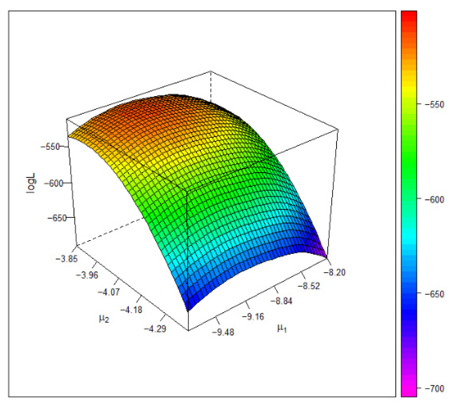
8.2. The Blood Pressure Data
9. Extension to Non-Normal Models
10. Conclusions
Author Contributions
Funding
Institutional Review Board Statement
Informed Consent Statement
Data Availability Statement
Acknowledgments
Conflicts of Interest
Appendix A
Appendix A.1. Proof of Lemma 1
Appendix A.2. Derivatives for Copulas
Appendix A.3. The Information Matrix under the Clayton Copula with Exponential Margins
References
- Gleser, L.J.; Olkin, L. Stochastically dependent effect sizes. In The Handbook of Research Synthesis; Russel Sage Foundation: New York, NY, USA, 1994. [Google Scholar]
- Riley, R.D. Multivariate meta-analysis: The effect of ignoring within-study correlation. J. R. Stat. Soc. Ser. A Stat. Soc. 2009, 172, 789–811. [Google Scholar] [CrossRef]
- Shih, J.-H.; Konno, Y.; Chang, Y.-T.; Emura, T. Estimation of a common mean vector in bivariate meta-analysis under the FGM copula. Statistics 2019, 53, 673–695. [Google Scholar] [CrossRef]
- Nissen, S.E.; Wolski, K. Effect of Rosiglitazone on the Risk of Myocardial Infarction and Death from Cardiovascular Causes. N. Engl. J. Med. 2007, 356, 2457–2471. [Google Scholar] [CrossRef] [PubMed] [Green Version]
- Yamaguchi, Y.; Maruo, K. Bivariate beta-binomial model using Gaussian copula for bivariate meta-analysis of two binary outcomes with low incidence. Jpn. J. Stat. Data Sci. 2019, 2, 347–373. [Google Scholar] [CrossRef] [Green Version]
- Mavridis, D.; Salanti, G. A practical introduction to multivariate meta-analysis. Stat. Methods Med. Res. 2011, 22, 133–158. [Google Scholar] [CrossRef]
- Copas, J.B.; Jackson, D.; White, I.; Riley, R.D. The role of secondary outcomes in multivariate meta-analysis. J. R. Stat. Soc. Ser. C Appl. Stat. 2018, 67, 1177–1205. [Google Scholar] [CrossRef]
- Burzykowski, T.; Molenberghs, G.; Buyse, M.; Geys, H.; Renard, D. Validation of surrogate end points in multiple randomized clinical trials with failure time end points. J. R. Stat. Soc. Ser. C Appl. Stat. 2001, 50, 405–422. [Google Scholar] [CrossRef] [Green Version]
- Rotolo, F.; Paoletti, X.; Michiels, S. surrosurv: An R package for the evaluation of failure time surrogate endpoints in individual patient data meta-analysis of randomized clinical trials. Comput. Methods Programs Biomed. 2018, 155, 189–198. [Google Scholar] [CrossRef]
- Rotolo, F.; Paoletti, X.; Burzykowski, T.; Buyse, M.; Michiels, S. A Poisson approach to the validation of failure time surrogate endpoints in individual patient data meta-analyses. Stat. Methods Med. Res. 2019, 28, 170–183. [Google Scholar] [CrossRef]
- Emura, T.; Sofeu, C.L.; Rondeau, V. Conditional copula models for correlated survival endpoints: Individual patient data meta-analysis of randomized controlled trials. Stat. Methods Med. Res. 2021, 30, 2634–2650. [Google Scholar] [CrossRef]
- Kuss, O.; Hoyer, A.; Solms, A. Meta-analysis for diagnostic accuracy studies: A new statistical model using beta-binomial dis-tributions and bivariate copulas. Stat. Med. 2014, 33, 17–30. [Google Scholar] [CrossRef]
- Nikoloulopoulos, A.K. A vine copula mixed effect model for trivariate meta-analysis of diagnostic test accuracy studies ac-counting for disease prevalence. Stat. Methods Med. Res. 2017, 26, 2270–2286. [Google Scholar] [CrossRef] [Green Version]
- Nikoloulopoulos, A.K. A D-vine copula mixed model for joint meta-analysis and comparison of diagnostic tests. Stat. Methods Med. Res. 2018, 28, 3286–3300. [Google Scholar] [CrossRef] [Green Version]
- Nikoloulopoulos, A.K. A multinomial quadrivariate D-vine copula mixed model for meta-analysis of diagnostic studies in the presence of non-evaluable subjects. Stat. Methods Med. Res. 2020, 29, 2988–3005. [Google Scholar] [CrossRef] [Green Version]
- Takeuchi, T.T. Constructing a bivariate distribution function with given marginals and correlation: Application to the galaxy luminosity function. Mon. Not. R. Astron. Soc. 2010, 406, 1830–1840. [Google Scholar] [CrossRef] [Green Version]
- Ota, S.; Kimura, M. Effective estimation algorithm for parameters of multivariate Farlie–Gumbel–Morgenstern copula. Jpn. J. Stat. Data Sci. 2021, 4, 1049–1078. [Google Scholar] [CrossRef]
- Ghosh, S.; Sheppard, L.W.; Holder, M.T.; Loecke, T.D.; Reid, P.C.; Bever, J.D.; Reuman, D.C. Copulas and their potential for ecology. Adv. Ecol. Res. 2020, 62, 409–468. [Google Scholar] [CrossRef]
- Alidoost, F.; Stein, A.; Su, Z. The use of bivariate copulas for bias correction of reanalysis air temperature data. PLoS ONE 2019, 14, e0216059. [Google Scholar] [CrossRef] [Green Version]
- Bhatti, M.I.; Do, H.Q. Recent development in copula and its applications to the energy, forestry and environmental sciences. Int. J. Hydrog. Energy 2019, 44, 19453–19473. [Google Scholar] [CrossRef]
- Emura, T.; Chen, Y.H. Analysis of Survival Data with Dependent Censoring: Copula-Based Approaches; JSS Research Series in Statistics; Springer: Singapore, 2018. [Google Scholar]
- Emura, T.; Matsui, S.; Rondeau, V. Survival Analysis with Correlated Endpoints, Joint Frailty-Copula Models; JSS Research Series in Statistics; Springer: Singapore, 2019. [Google Scholar]
- Emura, T.; Shih, J.-H.; Ha, I.D.; Wilke, R.A. Comparison of the marginal hazard model and the sub-distribution hazard model for competing risks under an assumed copula. Stat. Methods Med. Res. 2020, 29, 2307–2327. [Google Scholar] [CrossRef]
- Peng, M.; Xiang, L.; Wang, S. Semiparametric regression analysis of clustered survival data with semi-competing risks. Comput. Stat. Data Anal. 2018, 124, 53–70. [Google Scholar] [CrossRef]
- Huang, X.-W.; Wang, W.; Emura, T. A copula-based Markov chain model for serially dependent event times with a dependent terminal event. Jpn. J. Stat. Data Sci. 2020, 4, 917–951. [Google Scholar] [CrossRef]
- Shih, J.H. Common Mean. Copula: Bivariate Common Mean Vector under Copula Models; CRAN. 2022. Available online: https://CRAN.R-project.org/package=CommonMean.Copula (accessed on 8 January 2022).
- Berkey, C.S.; Hoaglin, D.C.; Antczak-bouckoms, A.; Mosteller, F.; Colditz, G.A. Meta-analysis of multiple outcomes by regression with random effect. Stat. Med. 1998, 17, 2537–2550. [Google Scholar] [CrossRef]
- Shinozaki, N. A note on estimating the common mean of k normal distributions and the stein problem. Commun. Stat.-Theory Methods 1978, 7, 1421–1432. [Google Scholar] [CrossRef]
- Malekzadeh, A.; Kharrati-Kopaei, M. Inferences on the common mean of several normal populations under hetero-scedasticity. Comput. Stat. 2018, 33, 1367–1384. [Google Scholar] [CrossRef]
- Gasparrini, A. Mvmeta: Multivariate and Univariate Meta-Analysis and Meta-Regression; CRAN. 2019. Available online: https://CRAN.R-project.org/package=mvmeta (accessed on 8 January 2022).
- Nelsen, R. An Introduction to Copulas. Technometrics. Lett. 2000, 42, 317. [Google Scholar] [CrossRef]
- Durante, F.; Sempi, C. Principles of Copula Theory; CRC/Chapman & Hall: Boca Raton, FL, USA, 2016. [Google Scholar]
- Morgenstern, D. Einfache Beispiele zweidimensionaler Verteilungen. Mitt. Für Math. Stat. 1956, 8, 34–235. [Google Scholar]
- Bairamov, I.G.; Kotz, S.; Bekci, M. New generalized Farlie-Gumbel-Morgenstern distributions and concomitants of order statistics. J. Appl. Stat. 2001, 28, 521–536. [Google Scholar] [CrossRef]
- Bairamov, I.; Kotz, S. Dependence structure and symmetry of Hunag-Kotz FGM distributions and their extensions. Metrika 2002, 56, 55–72. [Google Scholar] [CrossRef]
- Amini, M.; Jabbari, H.; Borzadaran, G.R.M. Aspects of Dependence in Generalized Farlie-Gumbel-Morgenstern Distributions. Commun. Stat.-Simul. Comput. 2011, 40, 1192–1205. [Google Scholar] [CrossRef]
- Domma, F.; Giordano, S. A copula-based approach to account for dependence in stress-strength models. Stat. Pap. 2012, 54, 807–826. [Google Scholar] [CrossRef]
- Chesneau, C. A new two-dimensional relation copula inspiring generalized version of the Farlie-Gumbel-Morgenstern copula. Res. Commun. Math. Math. Sci. 2021, 13, 99–128. [Google Scholar]
- Clayton, D.G. A model for association in bivariate life tables and its application in epidemiological studies of familial tendency in chronic disease incidence. Biometrika 1978, 65, 141–151. [Google Scholar] [CrossRef]
- Duchateau, L.; Janssen, P. The Frailty Model; Springer: New York, NY, USA, 2007. [Google Scholar]
- Gumbel, E.J. Distributions de valeurs extrêmes en plusieurs dimensions. Publ. Inst. Statist. Univ. Paris 1960, 9, 171–173. [Google Scholar]
- Frank, M.J. On the simultaneous associativity of F(x, y) and x+y−F(x, y). Aequ. Math. 1979, 19, 194–226. [Google Scholar] [CrossRef]
- Sklar, A. Fonctions de répartition à n dimensions et leurs marges. Publ. Inst. Statist. Univ. Paris 1959, 8, 229–231. [Google Scholar]
- Schucany, W.R.; Parr, W.C.; Boyer, J.E. Correlation structure in Farlie-Gumbel-Morgenstern distributions. Biometrika 1978, 65, 650–653. [Google Scholar] [CrossRef]
- Nelsen, R.B. Dependence and Order in Families of Archimedean Copulas. J. Multivar. Anal. 1997, 60, 111–122. [Google Scholar] [CrossRef] [Green Version]
- Bradley, R.A.; Gart, J.J. The asymptotic properties of ML estimators when sampling from associated populations. Biometrika 1962, 49, 205–214. [Google Scholar] [CrossRef]
- Emura, T.; Hu, Y.H.; Konno, Y. Asymptotic inference for maximum likelihood estimators under the special exponential family with double-truncation. Stat. Pap. 2017, 58, 877–909. [Google Scholar] [CrossRef]
- Shih, J.H. Copula-Based Statistical Inferences for a Common Mean Vector and Correlation Ratios Using Bivariate Data. Ph.D. Thesis, National Central University Library, Taoyuan, Taiwan, 2020. Available online: https://etd.lib.nctu.edu.tw/cgi-bin/gs32/ncugsweb.cgi/ccd=GLZeNP/record?r1=2&h1=2 (accessed on 3 October 2020).
- Shao, J. Mathematical Statistics; Springer: New York, NY, USA, 2003. [Google Scholar]
- Van der Vaart, A.W. Asymptotic Statistics; Cambridge University Press: Cambridge, UK, 1998. [Google Scholar]
- Lehmann, E.L.; Casella, G. Theory of Point Estimation, 2nd ed.; Springer: New York, NY, USA, 1998. [Google Scholar]
- Kontopantelis, E.; Reeves, D. Performance of statistical methods for meta-analysis when true study effects are non-normally distributed: A simulation study. Stat. Methods Med Res. 2010, 21, 409–426. [Google Scholar] [CrossRef]
- Jackson, D.; White, I.R.; Riley, R.D. A matrix-based method of moments for fitting the multivariate random effects model for meta-analysis and meta-regression. Biom. J. 2013, 55, 231–245. [Google Scholar] [CrossRef] [Green Version]
- Schepsmeier, U.; Stöber, J. Derivatives and Fisher information of bivariate copulas. Stat. Pap. 2013, 55, 525–542. [Google Scholar] [CrossRef]
- Oakes, D. A Model for Association in Bivariate Survival Data. J. R. Stat. Soc. Ser. B Stat. Methodol. 1982, 44, 414–422. [Google Scholar] [CrossRef]
- Nakatochi, M.; Kanai, M.; Nakayama, A.; Hishida, A.; Kawamura, Y.; Ichihara, S.; Matsuo, H. Genome-wide me-ta-analysis identifies multiple novel loci associated with serum uric acid levels in Japanese individuals. Commun. Biol. 2019, 2, 1–10. [Google Scholar] [CrossRef]
- Taketomi, N.; Konno, Y.; Chang, Y.-T.; Emura, T. A Meta-Analysis for Simultaneously Estimating Individual Means with Shrinkage, Isotonic Regression and Pretests. Axioms 2021, 10, 267. [Google Scholar] [CrossRef]
- Taketomi, N.; Michimae, H.; Chang, Y.-T.; Emura, T. meta.shrinkage: An R package for meta-analyses for simultaneously estimating individual means. Algorithms, 2022; accepted. [Google Scholar]


| Parameters | SD | SE | CP | SD | SE | CP | CP | |
|---|---|---|---|---|---|---|---|---|
| 5 | 0.064 | 0.046 | 0.888 | 0.042 | 0.033 | 0.885 | 0.859 | |
| 10 | 0.033 | 0.026 | 0.913 | 0.023 | 0.019 | 0.931 | 0.894 | |
| 15 | 0.021 | 0.019 | 0.933 | 0.015 | 0.014 | 0.936 | 0.919 | |
| 50 | 0.010 | 0.009 | 0.952 | 0.007 | 0.007 | 0.954 | 0.950 | |
| 100 | 0.007 | 0.006 | 0.955 | 0.005 | 0.005 | 0.943 | 0.944 | |
| 300 | 0.004 | 0.004 | 0.948 | 0.003 | 0.003 | 0.942 | 0.948 | |
| 5 | 0.105 | 0.092 | 0.938 | 0.100 | 0.086 | 0.920 | 0.909 | |
| 10 | 0.061 | 0.057 | 0.937 | 0.060 | 0.055 | 0.929 | 0.919 | |
| 15 | 0.049 | 0.045 | 0.938 | 0.045 | 0.042 | 0.943 | 0.930 | |
| 50 | 0.023 | 0.023 | 0.959 | 0.022 | 0.021 | 0.944 | 0.943 | |
| 100 | 0.016 | 0.016 | 0.942 | 0.015 | 0.015 | 0.957 | 0.950 | |
| 300 | 0.009 | 0.009 | 0.946 | 0.008 | 0.008 | 0.946 | 0.949 | |
| 5 | 0.115 | 0.105 | 0.932 | 0.128 | 0.120 | 0.935 | 0.922 | |
| 10 | 0.069 | 0.068 | 0.950 | 0.079 | 0.075 | 0.937 | 0.937 | |
| 15 | 0.058 | 0.053 | 0.941 | 0.062 | 0.058 | 0.947 | 0.937 | |
| 50 | 0.028 | 0.027 | 0.942 | 0.029 | 0.030 | 0.955 | 0.943 | |
| 100 | 0.019 | 0.019 | 0.942 | 0.021 | 0.020 | 0.936 | 0.945 | |
| 300 | 0.010 | 0.011 | 0.958 | 0.011 | 0.012 | 0.960 | 0.959 | |
| Year | Mean Math Score | Mean Stat Score | Covariance Matrix | Copula Parameter | |||||
|---|---|---|---|---|---|---|---|---|---|
| 1 | 2013 | 35.17 | 30.41 | 0.38 | 1.00 | 0.67 | 1.34 | 2.68 | |
| 2 | 2014 | 23.43 | 31.63 | 0.67 | 1.00 | 1.92 | 1.90 | 6.00 | |
| 3 | 2015 | 30.74 | 48.11 | 0.58 | 1.00 | 1.37 | 1.65 | 4.67 | |
| 4 | 2016 | 50.91 | 65.22 | 0.66 | 1.00 | 1.82 | 1.85 | 5.76 | |
| 5 | 2017 | 61.62 | 40.22 | 0.65 | 1.00 | 1.75 | 1.83 | 5.60 | |
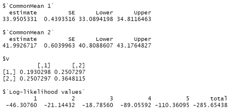
| Copula | Math: Estimate (95% CI) | Stat: Estimate (95% CI) | Log-likelihood | |
|---|---|---|---|---|
| FGM | 37.16 (35.85, 38.47) | 41.17 (39.65, 42.70) | −291.80 | 2723.91 |
| Clayton | 32.56 (31.71, 33.40) | 43.80 (42.55, 45.05) | −322.84 | 2644.03 |
| Gumbel | 37.67 (36.30, 39.03) | 42.56 (40.79, 44.33) | −279.28 | 2860.21 |
| Frank | 37.23 (35.97, 38.49) | 39.76 (38.13, 41.40) | −287.63 | 2738.09 |
| Normal | 35.83 (34.51, 37.16) | 38.64 (36.94, 40.34) | −342.65 | 2773.41 |
| Copula | SBP: Estimate (95% CI) | DBP: Estimate (95% CI) | Log-likelihood | |
|---|---|---|---|---|
| FGM | −9.18 (−9.32, −9.04) | −3.94 (−4.00, −3.89) | −530.29 | 177.23 |
| Clayton | −9.53 (−9.70, −9.36) | −4.34 (−4.38, −4.29) | −787.02 | 163.04 |
| Gumbel | −8.99 (−9.16, −8.83) | −3.94 (−4.00, −3.89) | −514.67 | 184.67 |
| Frank | −9.20 (−9.40, −9.00) | −3.94 (−3.99, −3.88) | −513.34 | 179.81 |
| Normal | −8.43 (−8.60, −8.25) | −3.95 (−4.01, −3.90) | −771.82 | 206.49 |
Publisher’s Note: MDPI stays neutral with regard to jurisdictional claims in published maps and institutional affiliations. |
© 2022 by the authors. Licensee MDPI, Basel, Switzerland. This article is an open access article distributed under the terms and conditions of the Creative Commons Attribution (CC BY) license (https://creativecommons.org/licenses/by/4.0/).
Share and Cite
Shih, J.-H.; Konno, Y.; Chang, Y.-T.; Emura, T. Copula-Based Estimation Methods for a Common Mean Vector for Bivariate Meta-Analyses. Symmetry 2022, 14, 186. https://doi.org/10.3390/sym14020186
Shih J-H, Konno Y, Chang Y-T, Emura T. Copula-Based Estimation Methods for a Common Mean Vector for Bivariate Meta-Analyses. Symmetry. 2022; 14(2):186. https://doi.org/10.3390/sym14020186
Chicago/Turabian StyleShih, Jia-Han, Yoshihiko Konno, Yuan-Tsung Chang, and Takeshi Emura. 2022. "Copula-Based Estimation Methods for a Common Mean Vector for Bivariate Meta-Analyses" Symmetry 14, no. 2: 186. https://doi.org/10.3390/sym14020186
APA StyleShih, J.-H., Konno, Y., Chang, Y.-T., & Emura, T. (2022). Copula-Based Estimation Methods for a Common Mean Vector for Bivariate Meta-Analyses. Symmetry, 14(2), 186. https://doi.org/10.3390/sym14020186