A Regularized Generalized Popov’s Method to Solve the Hierarchical Variational Inequality Problem with Generalized Lipschitzian Mappings

Abstract

In this article, we introduce a new inertial multi-step regularized generalized Popov’s extra-gradient method to solve the hierarchical variational inequality problem (HVIP). We extend the previous Lipschitzian and strongly monotone mapping to a hemicontinuous, generalized Lipschitzian and strongly monotone mapping. We also obtain a strong convergence theorem about the new Popov’s algorithm. Furthermore, we utilize some numerical experiments to highlight the feasibility and effectiveness of our method.

1. Introduction

Let $\mathcal{H}$ be a real Hilbert space, and $\mathcal{C}$ be a nonempty, closed, and convex subset of $\mathcal{H}$. The variational inequality problem is a fundamental nonlinear problem, which plays a significant role in engineering, economy, and control fields [1,2,3,4,5,6,7,8]. Specifically, it is to find a point $\tilde{y}\in \mathcal{C}$ such that

$$\langle A\tilde{y},w-\tilde{y}\rangle \ge 0,\forall w\in \mathcal{C},$$

(1)

where $A:\mathcal{H}\to \mathcal{H}$ is a mapping. We define $\mathrm{VI}(A,\mathcal{C})$ as the solution set of (1). In recent years, plenty of scholars have studied the hierarchical variational inequality problem (HVIP), which plays an important role in physical and practical issues, and so on. HVIP is to find a point $w^{*}\in \mathrm{VI}(A,\mathcal{C})$ such that

$$\langle F{w}^{*},z-w^{*}\rangle \ge 0,\forall z\in \mathrm{VI}(A,\mathcal{C}),$$

(2)

where mapping $A:\mathcal{C}\to \mathcal{H}$ is Lipschitzian and monotone, and mapping $F:\mathcal{H}\to \mathcal{H}$ is Lipschitzian and strongly monotone.

In order to study HVIP, many scholars proposed different iterative methods. The simplest iteration method is the projection algorithm,

$$w_{n+1}=P_{\mathcal{C}}(w_n-\lambda A{w}_n),$$

(3)

where $\lambda >0$, and mapping A is L-Lipschitzian and strongly monotone. However, if we want to establish the convergence of this algorithm, we should control the condition of A strictly. If A does not satisfy the strongly monotone condition, we will not obtain a strong convergence result, or even a weak convergence result. To weaken the conditions of A, Korpelevich [9] proposed the extra-gradient algorithm in which A is a Lipschitzian and monotone mapping. The algorithm is as follows:

$$\left\{\begin{array}{c}{z}_n=P_C(w_n-\lambda A{w}_n),\hfill \\ w_{n+1}=P_C(w_n-\lambda A{z}_n),\hfill \end{array}\right.$$

where $\lambda >0$. Afterwards, Popov [10] presented the following algorithm:

$$\left\{\begin{array}{c}{w}_{n+1}=P_{\mathcal{C}}(w_n-\lambda A{z}_n),\hfill \\ z_{n+1}=P_{\mathcal{C}}(w_{n+1}-\lambda A{z}_n),\hfill \end{array}\right.$$

where $\lambda \in \left(0,\frac{\sqrt{2}-1}{L}\right)$. Through observation, it is not difficult to find that Popov’s method only needs to compute the value of $z_n$ under the action of operator A at each iteration, but does not need to know the value of $w_n$ under the action of operator A. Therefore, compared with the extra-gradient method, the computation of Popov is reduced. However, Popov’s method still requires two projections on $\mathcal{C}$. If the spatial structure of $\mathcal{C}$ is intricate, then Popov’s method is also difficult to implement. In order to solve this problem, Malitsky et al. [11] proposed the following algorithm, which converts one of the projections on $\mathcal{C}$ into the projection on a half-space $T^n$,

$$\left\{\begin{array}{c}{T}^n=\{y\in \mathcal{H}:\langle w_n-\lambda A{z}_{n-1}-z_n,y-z_n\rangle \le 0\},\hfill \\ w_{n+1}=P_{T^n}(w_n-\lambda A{z}_n),\hfill \\ z_{n+1}=P_{\mathcal{C}}(w_{n+1}-\lambda A{z}_n),\hfill \end{array}\right.$$

(4)

where $\lambda \in \left(0,\frac{1}{3L}\right)$, mapping A is L-Lipschitzian and monotone. However, L is not always easy to obtain. In 2019, Hieu et al. [12] proposed a new step size, whose calculation is independent of the Lipschitz constant of A. The algorithm is as follows,

$$\left\{\begin{array}{cc}& T^n=\{w\in \mathcal{H}:\langle w_n-{\lambda }_{n}A{z}_{n-1}-z_n,w-z_n\rangle \le 0\},\hfill \\ & w_{n+1}=P_{T_n}(w_n-{\lambda }_{n}A{z}_n),\hfill \\ & z_{n+1}=P_{\mathcal{C}}(w_{n+1}-{\lambda }_{n+1}A{z}_n),\hfill \end{array}\right.$$

where

$${\lambda }_{n+1}=\left\{\begin{array}{cc}min\left\{{\lambda }_n,\frac{\mu \parallel z_{n-1}-z_n\parallel }{\parallel A{z}_n-A{z}_{n-1}\parallel }\right\},\hfill & \mathrm{if}A{z}_n\ne A{z}_{n-1},\hfill \\ {\lambda }_n,\hfill & \mathrm{otherwise},\hfill \end{array}\right.$$

and they established the weak convergence of $\left\{w_n\right\}$, $\left\{z_n\right\}$, which generated by the above algorithm.

The regularization method is an important method to solve VIP. Many scholars conducted a lot of research on the regularization method. In 2020, Hieu et al. [13] proposed regularization of Popov’s extra-gradient method (RPEGM) to solve HVIP ( 2). The proposed algorithm is given as

$$\left\{\begin{array}{c}{T}^n=\{y\in \mathcal{H}:\langle w_n-{\lambda }_n(A{z}_{n-1}+{\alpha }_{n}F{w}_n)-z_n,y-z_n\rangle \le 0\},\hfill \\ w_{n+1}=P_{T^n}[w_n-{\lambda }_n(A{z}_{n-1}+{\alpha }_{n}F{w}_n)],\hfill \\ z_{n+1}=P_{\mathcal{C}}[w_{n+1}-{\lambda }_{n+1}(A{z}_n+{\alpha }_{n+1}F{w}_{n+1})],\hfill \end{array}\right.$$

where

$${\lambda }_{n+1}=\left\{\begin{array}{cc}min\left\{{\lambda }_n,\frac{\mu \parallel z_{n-1}-z_n\parallel }{\parallel A{z}_n-A{z}_{n-1}\parallel }\right\},\hfill & \mathrm{if}A{z}_n\ne A{z}_{n-1},\hfill \\ {\lambda }_n,\hfill & \mathrm{otherwise}.\hfill \end{array}\right.$$

In recent years, many scholars studied HVIP (2) with the inertial method. Jiang et al. [14] proposed a new method (IRSEGM) for solving HVIP (2) with the hemicontinuous, generalized Lipschitzian and strongly monotone mapping, which combines multi-step inertial and regularization methods. The algorithm is as follows, and a strong convergence theorem is obtained when the parameters satisfy certain conditions:

$$\left\{\begin{array}{c}{u}_n=w_n+\sum _{i=1}^{min\{N,n\}}{\alpha }_{i,n}(w_{n-i+1}-w_{n-i}),\hfill \\ z_n=P_{\mathcal{C}}[u_n-{\lambda }_n(A{u}_n+{\beta }_{n}F{u}_n)],\hfill \\ T^n=\{w\in \mathcal{H}:\langle u_n-{\lambda }_n(A{u}_n+{\beta }_{n}F{u}_n)-z_n,w-z_n\rangle \le 0\},\hfill \\ w_{n+1}=P_{T^n}[u_n-{\lambda }_n(A{z}_n+{\beta }_{n}F{u}_n)],\hfill \end{array}\right.$$

(5)

where

$${\lambda }_{n+1}=\left\{\begin{array}{cc}min\left\{{\lambda }_n,\frac{\mu \parallel z_{n-1}-z_n\parallel }{\parallel A{z}_n-A{z}_{n-1}\parallel }\right\},\hfill & \mathrm{if}A{z}_n\ne A{z}_{n-1},\hfill \\ {\lambda }_n,\hfill & \mathrm{otherwise},\hfill \end{array}\right.$$

$${\alpha }_{i,n}=\left\{\begin{array}{cc}min\left\{{\alpha }_i,\frac{{\sigma }_{i,n}}{\parallel w_{n-i+1}-w_{n-i}\parallel }\right\},\hfill & \mathrm{if}{w}_{n-i+1}\ne w_{n-i},\hfill \\ {\lambda }_n,\hfill & \mathrm{otherwise},\hfill \end{array}\right.$$

N is a chosen positive integer, mapping A is L-Lipschitzian and monotone, and mapping F is hemicontinuous, generalized Lipschitzian and strongly monotone.

In this article, motivated by the above results, we propose a new multi-step inertial regularized generalized Popov’s extra-gradient method for the sake of accelerating the convergence of sequences. On the basis of previous studies, we extend F in HVIP (2) to the hemicontinuous and generalized Lipschitzian. Finally, we obtain the strong convergence result of our new algorithm under the suitable conditions. The structure of our paper is as follows. In the first part, we mainly give some of the research background. In the second part, we introduce some important definitions and lemmas. In the third part, we present a new method to deal with HVIP (2), combining the multi-step inertial regularization method with Popov’s extra-gradient method in Hilbert space, and get a strong convergence theorem for our algorithm involving mapping F as hemicontinuous, generalized Lipschitzian and strongly monotone. In the last part, numerical examples are used to exhibit the validity of our algorithm.

2. Preliminaries

In this part, we give some significant lemmas and definitions, which are important for the rest of the proof.

We respectively use → to represent strong convergence and ⇀ to represent weak convergence.

Definition 1

([14,15]). Let $A:\mathcal{H}\to \mathcal{H}$ be a mapping.

(i) 

If mapping A satisfies

$$\langle Aw-Az,w-z\rangle \ge 0,\forall w,z\in \mathcal{H}.$$

then A is monotone.

(ii) 

If for $\eta >0$, mapping A satisfies

$$\langle Aw-Az,w-z\rangle \ge {\eta \parallel w-z\parallel }^2,\forall w,z\in \mathcal{H},$$

then A is η-strongly monotone.

(iii) 

If for $L>0$, mapping A satisfies

$$\parallel Aw-Az\parallel \le L\parallel w-z\parallel ,\forall w,z\in \mathcal{H},$$

then A is L-Lipschitzian.

(iv) 

If for $L>0$, mapping A satisfies

$$\parallel Aw-Az\parallel \le L(\parallel w-z\parallel +1),\forall w,z\in \mathcal{H},$$

then A is L-generalized Lipschitzian.

(v) 

A is hemicontinuous if

$$\forall w,h\in \mathcal{H},t_n\to 0\Rightarrow A(w+t_{n}h)\rightharpoonup Aw\mathrm{as}n\to \infty .$$

Remark 1.

According to the definition of Lipschitzian and generalized Lipschitzian, it is not difficult to find that the generalized Lipschitzian is broader than Lipschitzian. In fact, the generalized Lipschitzian is not even necessarily hemicontinuous. A specific example is as follows.

Example 1.

Let $g:\mathbb{R}\to \mathbb{R}$, and

$$g\left(w\right)=\left\{\begin{array}{cc}w-1,\hfill & w<-1,\hfill \\ w-\sqrt{1-{(w+1)}^2},\hfill & -1\le w\le 0,\hfill \\ w+\sqrt{1-{(w-1)}^2},\hfill & 0\le w\le 1,\hfill \\ w+1,\hfill & w>1.\hfill \end{array}\right.$$

Through simple proofs, it is not difficult to show that $g\left(w\right)$ is generalized Lipschitzian, but it is clearly not Lipschitzian. Therefore, the algorithm proposed by us is valuable and meaningful. Other examples can be found in the literature ([14,16]).

Lemma 1

([16]). Supposing that the mapping $A:\mathcal{H}\to \mathcal{H}$ is hemicontinous and strongly monotone in VIP (1), then VIP (1) has one and only one solution.

Lemma 2

([17,18]). If for any $w\in \mathcal{H}$, there is one and only one element $q\in \mathcal{C}$ that meets $\parallel w-q\parallel \le \parallel w-z\parallel$, for any $y\in \mathcal{C}$, in that way we denote that $q=P_{\mathcal{C}}w$, where $\mathcal{H}$ is a real Hilbert space, $\mathcal{C}$ is a nonempty closed convex subset of the $\mathcal{H}$, and we have

$$q=P_{\mathcal{C}}w\iff \langle w-q,z-q\rangle \le 0,\forall z\in \mathcal{C}.$$

Lemma 3

([19]). Let $\left\{b_n\right\}$ be a non-negative real sequence such that

$$b_{n+1}\le (1-{\kappa }_n)b_n+{\kappa }_n{\sigma }_n+{\delta }_n,n=1,2,\dots ,$$

where $\left\{{\kappa }_n\right\}$, $\left\{{\sigma }_n\right\}$ and $\left\{{\delta }_n\right\}$ meet the following criteria respectively:

(i) 

$\left\{{\kappa }_n\right\}\subset (0,1)$;

(ii) 

${\sum }_{n=1}^{\infty }{\kappa }_n=\infty$;

(iii) 

$lim\; sup{\sigma }_n\le 0$;

(iv) 

${\sum }_{n=1}^{\infty }\left|{\delta }_n\right|<\infty$.

Then, ${lim}_{n\to \infty }{b}_n=0$.

3. Main Results

In this part, we raise a new method to deal with HVIP (2), which combines the multi-step inertia method with the regularization technique in Popov’s extra-gradient method. Through a series of derivations and proofs, the main result of our paper is obtained. Next, we assume that our algorithm satisfies the following conditions:

(${\mathrm{C}}_1$)

A is k-Lipschitzian on $\mathcal{H}$ and monotone on $\mathcal{C}$.

(${\mathrm{C}}_2$)

F is hemicontinuous, $\beta$-generalized Lipschitzian and $\gamma$-strongly monotone on $\mathcal{H}$.

(${\mathrm{C}}_3$)

The solution set $\mathrm{VI}(A,\mathcal{C})$ is nonempty.

(${\mathrm{C}}_4$)

Let $\left\{{\alpha }_n\right\}$ be a sequence of $(0,\infty )$ and meet ${\sum }_{n=1}^{\infty }{\alpha }_n=\infty$, ${\sum }_{n=1}^{\infty }{\alpha }_n^2<\infty$, ${lim}_{n\to \infty }\frac{{\alpha }_{n+1}-{\alpha }_n}{{\alpha }_n^2}$$=0$.

(${\mathrm{C}}_5$)

Let $\left\{{\sigma }_{i,n}\right\}$ be a sequence and satisfy $\left\{{\sigma }_{i,n}\right\}\subset (0,\infty )$, ${lim}_{n\to \infty }\frac{{\sigma }_{i,n}}{{\alpha }_n}=0$, ${\sum }_{n=1}^{\infty }{\sigma }_{i,n}<\infty$, where $i=1,2,3,\cdots ,N$ (where N is a chosen positive integer).

Remark 2.

In condition (${\mathrm{C}}_4$), we can take ${\alpha }_n=n^{-p}$, where $\frac{1}{2}<p<1$.

Now, we represent our new multi-step inertial regularized generalized Popov’s extra-gradient method.

Lemma 4.

The sequence $\left\{{\lambda }_n\right\}$ generated by our Algorithm 1 is not increasing, and ${lim}_{n\to \infty }{\lambda }_n\ge min\{{\lambda }_1$, $\frac{\mu }{k}\}>0$.

Algorithm 1: The multi-step inertial regularized generalized Popov’s extra-gradient method.

Initialization: Given ${\lambda }_0$, ${\lambda }_1$, ${\alpha }_0>0$, $\mu \in (0,\sqrt{2}-1)$. Let $w_0$, $z_0$, $u_0$ be any three members of $\mathcal{H}$. Step 1. Compute $$w_1=P_{\mathcal{C}}[u_0-{\lambda }_0(A{z}_0+{\alpha }_{0}F{u}_0)],$$ $$u_1=w_1+{\theta }_{1,1}(w_1-w_0),$$ $$z_1=P_{\mathcal{C}}[u_1-{\lambda }_1(A{z}_0+{\alpha }_{1}F{u}_1)].$$ Step 2. Given the current iterate $w_n$, $z_n$, and $z_{n-1}$, compute $w_{n+1}$ as follows: $$T^n=\{w\in \mathcal{H}:\langle u_n-{\lambda }_n(A{z}_{n-1}+{\alpha }_{n}F{u}_n)-z_n,w-z_n\rangle \le 0\}.$$ $$w_{n+1}=P_{T^n}[u_n-{\lambda }_n(A{z}_n+{\alpha }_{n}F{u}_n)],$$ Step 3. Compute $$u_{n+1}=w_{n+1}+\sum _{i=1}^{min\{N,n+1\}}{\theta }_{i,n+1}(w_{n+2-i}-w_{n+1-i}),$$ $$z_{n+1}=P_{\mathcal{C}}[u_{n+1}-{\lambda }_{n+1}(A{z}_n+{\alpha }_{n+1}F{u}_{n+1})].$$  where $0<{\theta }_{i,n}<{\theta }_i$, for some ${\theta }_i\in \mathcal{H}$ with $${\theta }_{i,n}=\left\{\begin{array}{cc}min\left\{{\theta }_i,\frac{{\sigma }_{i,n}}{\parallel w_{n+1-i}-w_{n-i}\parallel }\right\},\hfill & \mathrm{if}{w}_{n+1-i}\ne w_{n-i},\hfill \\ {\theta }_i,\hfill & \mathrm{otherwise},\hfill \end{array}\right.$$ $${\lambda }_{n+1}=\left\{\begin{array}{cc}min\left\{{\lambda }_n,\frac{\mu \parallel z_{n-1}-z_n\parallel }{\parallel A{z}_n-A{z}_{n-1}\parallel }\right\},\hfill & \mathrm{if}A{z}_n\ne A{z}_{n-1},\hfill \\ {\lambda }_n,\hfill & \mathrm{otherwise}.\hfill \end{array}\right.$$ Step 4. Set $n:=n+1$ and go to Step 1.

Proof. 

By definition of the sequence $\left\{{\lambda }_n\right\}$, it is obvious that the sequence $\left\{{\lambda }_n\right\}$ is not increasing. Since A is k-Lipschitz continuous with $k\ge 0$, we have

$$\parallel Aw-Az\parallel \le k\parallel w-z\parallel ,\forall w,z\in \mathcal{H}$$

In the case of $A{z}_n\ne A{z}_{n-1}$, we have

$$\frac{\mu \parallel z_{n-1}-z_n\parallel }{\parallel A{z}_n-A{z}_{n-1}\parallel }\ge \frac{\mu \parallel z_{n-1}-z_n\parallel }{k\parallel z_n-z_{n-1}\parallel }=\frac{\mu }{k}.$$

Clearly, the lower bound of the sequence $\left\{{\lambda }_n\right\}$ is $min\{{\lambda }_1,\frac{\mu }{k}\}$. □

By conditions $\left({\mathrm{C}}_1\right)$–$\left({\mathrm{C}}_3\right)$, we can easily see that $(A+\alpha F)$ is hemicontinous and strongly monotone. Therefore, in the light of Lemma 1, it is easy to conclude that for each $\alpha >0$, there is only one solution $w_{\alpha }$ for the following variational problem (6).

$$\mathrm{Find}z\in \mathcal{C},\mathrm{such}\mathrm{that}\langle (A+\alpha F)z,w-z\rangle \ge 0,\forall w\in \mathcal{C},$$

(6)

where $\alpha >0$. In the same way, for every $n\in \mathbb{N}$, there is a unique member $w_{{\alpha }_n}\in \mathcal{C}$ that makes

$$\langle (A+{\alpha }_{n}F)w_{{\alpha }_n},w-w_{{\alpha }_n}\rangle \ge 0,\forall w\in \mathcal{C}.$$

(7)

On the other hand, according to Lemma 1, it is easy to find that when conditions $\left({\mathrm{C}}_1\right)$–$\left({\mathrm{C}}_3\right)$ are satisfied, there is a unique solution $w^{*}$ to HVIP (2).

Lemma 5

([14]). For $w_{\alpha }$ and $w^{*}$ above, we have the following:

(i) 

For all $\mu ,\nu >0,\parallel w_{\mu }-w_{\nu }\parallel \le \frac{|\mu -\nu |}{\mu }\tau$, where τ is a positive constant,

$$\tau =\frac{1}{\gamma }\left[\left(1+\frac{\beta }{\gamma }\right)\parallel F{w}^{*}\parallel +2\beta \parallel w^{*}\parallel +\beta \right].$$

(ii) 

$\left\{w_{\alpha }\right\}$ is bounded, and $\parallel w_{\alpha }\parallel \le \frac{1}{\eta }\parallel F{w}^{*}\parallel +\parallel w^{*}\parallel$.

(iii) 

${lim}_{\alpha \to 0^{+}}{w}_{\alpha }=w^{*}$.

Lemma 6.

For all $n+1\ge N$,

$$\parallel u_{n+1}-z_n{\parallel }^2\le \left(1+\sum _{i=1}^N{\sigma }_{i,n+1}\right){\parallel w_{n+1}-z_n\parallel }^2+{\overline{\sigma }}_{n+1},$$

where${\overline{\sigma }}_{n+1}={\sum }_{i=1}^N{\sigma }_{i,n+1}^2+2{\sum }_{1\le i<j\le N}{\sigma }_{i,n+1}{\sigma }_{j,n+1}+{\sum }_{i=1}^N{\sigma }_{i,n+1}$.

Proof. 

By the definition of $u_n$, we deduce

$$\begin{array}{ccc}& & \parallel u_{n+1}-z_n{\parallel }^2\hfill \\ & =& {∥(w_{n+1}-z_n)+\sum _{i=1}^N{\theta }_{i,n+1}(w_{n+2-i}-w_{n+1-i})∥}^2\hfill \\ & \le & {\left(\parallel w_{n+1}-z_n\parallel +\sum _{i=1}^N{\theta }_{i,n+1}\parallel w_{n+2-i}-w_{n+1-i}\parallel \right)}^2\hfill \\ & =& \parallel w_{n+1}-z_n{\parallel }^2+\sum _{i=1}^N{\theta }_{i,n+1}^2{\parallel w_{n+2-i}-w_{n+1-i}\parallel }^2\hfill \\ & & +2\parallel w_{n+1}-z_n\parallel \sum _{i=1}^N{\theta }_{i,n+1}\parallel w_{n+2-i}-w_{n+1-i}\parallel \hfill \\ & & +2\sum _{1\le i<j\le N}{\theta }_{i,n+1}{\theta }_{j,n+1}\parallel w_{n+2-i}-w_{n+1-i}\parallel \parallel w_{n+2-j}-w_{n+1-j}\parallel \hfill \\ & \le & \parallel w_{n+1}-z_n{\parallel }^2+\sum _{i=1}^N{\sigma }_{i,n+1}^2+{\parallel w_{n+1}-z_n\parallel }^2\sum _{i=1}^N{\sigma }_{i,n+1}\hfill \\ & & +\sum _{i=1}^N{\sigma }_{i,n+1}+2\sum _{1\le i<j\le N}{\sigma }_{i,n+1}{\sigma }_{j,n+1}\hfill \\ & =& \left(1+\sum _{i=1}^N{\sigma }_{i,n+1}\right){\parallel w_{n+1}-z_n\parallel }^2+{\overline{\sigma }}_{n+1}.\hfill \end{array}$$

□

Lemma 7.

Let m and n be two arbitrary real numbers and a be an arbitrary positive real number, then we have

(i) 

$mn\le \frac{1}{2}\left(a{m}^2+\frac{1}{a}{n}^2\right)$,

(ii) 

${(m+n)}^2\le (2+\sqrt{2})m^2+\sqrt{2}{n}^2$.

Proof. 

(i) Since ${(n-am)}^2=n^2-2amn+a^2{m}^2\ge 0$, we get $2amn\le n^2+a^2{m}^2$, so we deduce

$$mn\le \frac{1}{2}\left(a{m}^2+\frac{1}{a}{n}^2\right).$$

Peculiarly, taking $a=\sqrt{2}$, then we obtain $mn\le \frac{1}{2}\left(\sqrt{2}{m}^2+\frac{1}{\sqrt{2}}{n}^2\right)$.

(ii) Taking $a=1+\sqrt{2}$ in (i), we have

$$2mn\le (1+\sqrt{2})m^2+(\sqrt{2}-1)n^2,$$

then we deduce

$${(m+n)}^2\le (2+\sqrt{2})m^2+\sqrt{2}{n}^2.$$

□

Theorem 1.

Assuming that Algorithm 3.1 satisfies condition $\left({\mathrm{C}}_1\right)$–$\left({\mathrm{C}}_5\right)$, then the sequence $\left\{w_n\right\}$ produced by the algorithm strongly converges to the unique solution $w^{*}$ of HVIP (2).

Proof. 

According to Lemma 5, we have $w_{{\alpha }_n}\to w^{*}$. So we just have to prove $\parallel w_{{\alpha }_n}-w_n\parallel \to 0$ to get $w_{{\alpha }_n}\to w^{*}$, and the proof is as follows. Since

$$\begin{array}{ccc}& & \parallel u_n-w_{{\alpha }_n}{\parallel }^2\hfill \\ & =& \parallel u_n-w_{n+1}{\parallel }^2+{\parallel w_{n+1}-w_{{\alpha }_n}\parallel }^2+2\langle u_n-w_{n+1},w_{n+1}-w_{{\alpha }_n}\rangle ,\hfill \end{array}$$

from (7), we have

$$\begin{array}{ccc}& & \parallel w_{{\alpha }_n}-w_{n+1}{\parallel }^2\hfill \\ & =& \parallel u_n-w_{{\alpha }_n}{\parallel }^2-2\langle w_{n+1}-u_n,w_{{\alpha }_n}-w_{n+1}\rangle -{\parallel u_n-w_{n+1}\parallel }^2\hfill \\ & =& \parallel u_n-w_{{\alpha }_n}{\parallel }^2-2\langle w_{n+1}-u_n,w_{{\alpha }_n}-w_{n+1}\rangle -{\parallel (w_{n+1}-z_n)+(z_n-u_n)\parallel }^2\hfill \\ & =& \parallel u_n-w_{{\alpha }_n}{\parallel }^2-2\langle w_{n+1}-u_n,w_{{\alpha }_n}-w_{n+1}\rangle -\parallel w_{n+1}-z_n{\parallel }^2-{\parallel u_n-z_n\parallel }^2\hfill \\ & & -2\langle w_{n+1}-z_n,z_n-u_n\rangle \hfill \\ & =& \parallel u_n-w_{{\alpha }_n}{\parallel }^2-\parallel w_{n+1}-z_n{\parallel }^2-{\parallel u_n-z_n\parallel }^2\hfill \\ & & +2\langle u_n-{\lambda }_n(A{z}_{n-1}+{\alpha }_{n}F{u}_n)-z_n,w_{n+1}-z_n\rangle \hfill \\ & & +2\langle u_n-{\lambda }_n(A{z}_n+{\alpha }_{n}F{u}_n)-w_{n+1},w_{{\alpha }_n}-w_{n+1}\rangle \hfill \\ & & +2{\lambda }_n\langle A{z}_{n-1}+{\alpha }_{n}F{u}_n,w_{n+1}-z_n\rangle +2{\lambda }_n\langle A{z}_n+{\alpha }_{n}F{u}_n,w_{{\alpha }_n}-w_{n+1}\rangle \hfill \\ & =& \parallel u_n-w_{{\alpha }_n}{\parallel }^2-\parallel w_{n+1}-z_n{\parallel }^2-{\parallel u_n-z_n\parallel }^2\hfill \\ & & +2\langle u_n-{\lambda }_n(A{z}_{n-1}+{\alpha }_{n}F{u}_n)-z_n,w_{n+1}-z_n\rangle \hfill \\ & & +2\langle u_n-{\lambda }_n(A{z}_n+{\alpha }_{n}F{u}_n)-w_{n+1},w_{{\alpha }_n}-w_{n+1}\rangle \hfill \\ & & +2{\lambda }_n\langle A{z}_{n-1}-A{z}_n+A{z}_n+{\alpha }_{n}F{u}_n,w_{n+1}-z_n\rangle \hfill \\ & & +2{\lambda }_n\langle A{z}_n+{\alpha }_{n}F{u}_n,w_{{\alpha }_n}-w_{n+1}\rangle \hfill \\ & =& \parallel u_n-w_{{\alpha }_n}{\parallel }^2-\parallel w_{n+1}-z_n{\parallel }^2-{\parallel u_n-z_n\parallel }^2\hfill \\ & & +2\langle u_n-{\lambda }_n(A{z}_{n-1}+{\alpha }_{n}F{u}_n)-z_n,w_{n+1}-z_n\rangle \hfill \\ & & +2\langle u_n-{\lambda }_n(A{z}_n+{\alpha }_{n}F{u}_n)-w_{n+1},w_{{\alpha }_n}-w_{n+1}\rangle \hfill \\ & & +2{\lambda }_n\langle A{z}_n+{\alpha }_{n}F{u}_n,w_{{\alpha }_n}-z_n\rangle +2{\lambda }_n\langle A{z}_{n-1}-A{z}_n,w_{n+1}-z_n\rangle .\hfill \end{array}$$

By the definition of $w_{n+1}$ and $T^n$, we have

$$2\langle u_n-{\lambda }_n(A{z}_{n-1}+{\alpha }_{n}F{u}_n)-z_n,w_{n+1}-z_n\rangle \le 0.$$

(8)

Similarly, by the definition of $w_{n+1}$, Lemma 2, and $w_{{\alpha }_n}\in \mathcal{C}\subset T^n$, we also have

$$\langle u_n-{\lambda }_n(A{z}_n+{\alpha }_{n}F{u}_n)-w_{n+1},w_{{\alpha }_n}-w_{n+1}\rangle \le 0.$$

(9)

Combining (8) and (9), we obtain

$$\begin{array}{ccc}\hfill & & \parallel w_{{\alpha }_n}-w_{n+1}{\parallel }^2\hfill \\ & \le & \parallel u_n-w_{{\alpha }_n}{\parallel }^2-\parallel w_{n+1}-z_n{\parallel }^2-{\parallel u_n-z_n\parallel }^2\hfill \\ & & +2{\lambda }_n\langle A{z}_n+{\alpha }_{n}F{u}_n,w_{{\alpha }_n}-z_n\rangle +2{\lambda }_n\langle A{z}_{n-1}-A{z}_n,w_{n+1}-z_n\rangle .\hfill \end{array}$$

(10)

Now let us think about $2{\lambda }_n\langle A{z}_{n-1}-A{z}_n,w_{n+1}-z_n\rangle$ and $2{\lambda }_n\langle A{z}_n+{\alpha }_{n}F{u}_n,w_{{\alpha }_n}-z_n\rangle$. According to the definition of $\left\{{\lambda }_n\right\}$ and Lemma 7, we have

$$\begin{array}{ccc}\hfill & & 2{\lambda }_n\langle A{z}_{n-1}-A{z}_n,w_{n+1}-z_n\rangle \hfill \\ & \le & 2{\lambda }_n\parallel A{z}_n-A{z}_{n-1}\parallel \parallel w_{n+1}-z_n\parallel \hfill \\ & \le & \frac{2{\lambda }_n\mu }{{\lambda }_{n+1}}\parallel z_n-z_{n-1}\parallel \parallel w_{n+1}-z_n\parallel \hfill \\ & \le & \frac{{\lambda }_n\mu }{{\lambda }_{n+1}}\left(\frac{1}{\sqrt{2}}\parallel z_n-z_{n-1}{\parallel }^2+\sqrt{2}{\parallel w_{n+1}-z_n\parallel }^2\right)\hfill \\ & \le & \frac{{\lambda }_n\mu }{{\lambda }_{n+1}}\left[\frac{1}{\sqrt{2}}\parallel (z_n-u_n)+(u_n-z_{n-1}){\parallel }^2+\sqrt{2}{\parallel w_{n+1}-z_n\parallel }^2\right]\hfill \\ & \le & \frac{{\lambda }_n\mu }{{\lambda }_{n+1}}\left\{\frac{1}{\sqrt{2}}\left[(2+\sqrt{2})\parallel z_n-u_n{\parallel }^2+\sqrt{2}{\parallel u_n-z_{n-1}\parallel }^2\right]+\sqrt{2}{\parallel w_{n+1}-z_n\parallel }^2\right\}\hfill \\ & \le & \frac{(1+\sqrt{2}){\lambda }_n\mu }{{\lambda }_{n+1}}\parallel u_n-z_n{\parallel }^2+\frac{{\lambda }_n\mu }{{\lambda }_{n+1}}{\parallel u_n-z_{n-1}\parallel }^2\hfill \\ & & +\frac{\sqrt{2}{\lambda }_n\mu }{{\lambda }_{n+1}}{\parallel w_{n+1}-z_n\parallel }^2.\hfill \end{array}$$

(11)

Next, we consider $2{\lambda }_n\langle A{z}_n+{\alpha }_{n}F{u}_n,w_{{\alpha }_n}-z_n\rangle$. Since ${\alpha }_n\to 0$ and $\frac{{\sigma }_{i,n+1}}{{\alpha }_{n+1}}\to 0$ for each $i=1,2,\cdots ,N$, let ${\xi }_1$, ${\xi }_2$, ${\xi }_3$ be three positive real numbers and satisfy

$$2\gamma -\beta {\xi }_1-{\xi }_2-{\xi }_3>0,$$

$$\sum _{i=1}^N{\sigma }_{i,n}\le {\xi }_3{\lambda }_n{\alpha }_n,\forall n\ge n_0.$$

From Lemma 4, it is not difficult to know that there is a constant c that makes $0<c\le {\lambda }_n\le {\lambda }_1$. So with ${\alpha }_n\to 0$ as $n\to \infty$, we obtain $\frac{{\lambda }_n{\alpha }_n\beta }{{\xi }_1}\to 0$. On the other hand, from Lemma 4, we have $\frac{(1+\sqrt{2})\mu {\lambda }_n}{{\lambda }_{n+1}}\to (1+\sqrt{2})\mu$. Since $\mu \in (0,\sqrt{2}-1)$, without loss of generality, we have

$$1-\frac{(1+\sqrt{2}){\lambda }_n\mu }{{\lambda }_{n+1}}-\frac{{\lambda }_n{\alpha }_n\beta }{{\xi }_1}-{\xi }_2>0,\forall n\ge n_0.$$

(12)

Due to $w_{{\alpha }_n}\in \mathrm{VI}(A+{\alpha }_{n}F,\mathcal{C})$, $z_n\in \mathcal{C}$, we have

$$\langle A{w}_{{\alpha }_n}+{\alpha }_{n}F{w}_{{\alpha }_n},w_{{\alpha }_n}-z_n\rangle \le 0.$$

(13)

Combining the conditions $\left({\mathrm{C}}_1\right)$ and $\left({\mathrm{C}}_2\right)$, we abtain

$$\begin{array}{ccc}\hfill & & 2{\lambda }_n\langle A{z}_n+{\alpha }_{n}F{u}_n,w_{{\alpha }_n}-z_n\rangle \hfill \\ & =& 2{\lambda }_n\langle A{z}_n-A{w}_{{\alpha }_n},w_{{\alpha }_n}-z_n\rangle +2{\lambda }_n\langle A{w}_{{\alpha }_n}+{\alpha }_{n}F{u}_n,w_{{\alpha }_n}-z_n\rangle \hfill \\ & \le & 2{\lambda }_n\langle A{w}_{{\alpha }_n}+{\alpha }_{n}F{u}_n,w_{{\alpha }_n}-z_n\rangle \hfill \\ & =& 2{\lambda }_n\langle A{w}_{{\alpha }_n}+{\alpha }_{n}F{w}_{{\alpha }_n},w_{{\alpha }_n}-z_n\rangle +2{\lambda }_n\langle {\alpha }_{n}F{u}_n-{\alpha }_{n}F{w}_{{\alpha }_n},w_{{\alpha }_n}-z_n\rangle \hfill \\ & \le & 2{\lambda }_n\langle {\alpha }_{n}F{u}_n-{\alpha }_{n}F{w}_{{\alpha }_n},w_{{\alpha }_n}-z_n\rangle \hfill \\ & =& 2{\lambda }_n\langle {\alpha }_{n}F{u}_n-{\alpha }_{n}F{w}_{{\alpha }_n},w_{{\alpha }_n}-u_n\rangle +2{\lambda }_n\langle {\alpha }_{n}F{u}_n-{\alpha }_{n}F{w}_{{\alpha }_n},u_n-z_n\rangle \hfill \\ & \le & -2{\lambda }_n{\alpha }_n\gamma {\parallel u_n-w_{{\alpha }_n}\parallel }^2+2{\lambda }_n\langle {\alpha }_{n}F{u}_n-{\alpha }_{n}F{w}_{{\alpha }_n},u_n-z_n\rangle \hfill \\ & \le & -2{\lambda }_n{\alpha }_n\gamma \parallel u_n-w_{{\alpha }_n}{\parallel }^2+2{\lambda }_n{\alpha }_n\parallel F{u}_n-F{w}_{{\alpha }_n}\parallel \parallel u_n-z_n\parallel \hfill \\ & \le & -2{\lambda }_n{\alpha }_n\gamma \parallel u_n-w_{{\alpha }_n}{\parallel }^2+2{\lambda }_n{\alpha }_n\beta (\parallel u_n-w_{{\alpha }_n}\parallel +1)\parallel u_n-z_n\parallel \hfill \\ & =& -2{\lambda }_n{\alpha }_n\gamma \parallel u_n-w_{{\alpha }_n}{\parallel }^2+2{\lambda }_n{\alpha }_n\beta \parallel u_n-w_{{\alpha }_n}\parallel \parallel u_n-z_n\parallel \hfill \\ & & +2{\lambda }_n{\alpha }_n\beta \parallel u_n-z_n\parallel \hfill \\ & \le & -2{\lambda }_n{\alpha }_n\gamma {\parallel u_n-w_{{\alpha }_n}\parallel }^2+2{\lambda }_n{\alpha }_n\beta \left(\frac{1}{2}{\xi }_1\parallel u_n-w_{{\alpha }_n}{\parallel }^2+\frac{1}{2{\xi }_1}{\parallel u_n-z_n\parallel }^2\right)\hfill \\ & & +2\left(\frac{1}{2}{\xi }_2{\parallel u_n-z_n\parallel }^2+\frac{{\lambda }_n^2{\alpha }_n^2{\beta }^2}{2{\xi }_2}\right)\hfill \\ & =& -(2\gamma -{\xi }_1\beta ){\lambda }_n{\alpha }_n\parallel u_n-w_{{\alpha }_n}{\parallel }^2+\left(\frac{{\lambda }_n{\alpha }_n\beta }{{\xi }_1}+{\xi }_2\right){\parallel u_n-z_n\parallel }^2\hfill \\ & & +\frac{{\lambda }_n^2{\alpha }_n^2{\beta }^2}{{\xi }_2}.\hfill \end{array}$$

(14)

Substituting (11) and (14) into (10), we deduce

$$\begin{array}{ccc}\hfill & & \parallel w_{{\alpha }_n}-w_{n+1}{\parallel }^2\hfill \\ & \le & \parallel u_n-w_{{\alpha }_n}{\parallel }^2-\parallel w_{n+1}-z_n{\parallel }^2-{\parallel u_n-z_n\parallel }^2\hfill \\ & & +2{\lambda }_n\langle A{z}_{n-1}-A{z}_n,w_{n+1}-z_n\rangle +2{\lambda }_n\langle A{z}_n+{\alpha }_{n}F{u}_n,w_{{\alpha }_n}-z_n\rangle \hfill \\ & \le & \left[1-(2\gamma -{\xi }_1\beta ){\lambda }_n{\alpha }_n\right]\parallel u_n-w_{{\alpha }_n}{\parallel }^2-\left(1-\frac{\sqrt{2}{\lambda }_n\mu }{{\lambda }_{n+1}}\right){\parallel w_{n+1}-z_n\parallel }^2\hfill \\ & & -\left[1-\frac{(1+\sqrt{2}){\lambda }_n\mu }{{\lambda }_{n+1}}-\frac{{\lambda }_n{\alpha }_n\beta }{{\xi }_1}-{\xi }_2\right]{\parallel u_n-z_n\parallel }^2\hfill \\ & & +\frac{{\lambda }_n\mu }{{\lambda }_{n+1}}{\parallel u_n-z_{n-1}\parallel }^2+\frac{{\lambda }_n^2{\alpha }_n^2{\beta }^2}{{\xi }_2}.\hfill \end{array}$$

(15)

Combining (12) and (15), for all $n\ge n_0$, we have

$$\begin{array}{ccc}\hfill & & \parallel w_{{\alpha }_n}-w_{n+1}{\parallel }^2\hfill \\ & \le & \left[1-(2\gamma -{\xi }_1\beta ){\lambda }_n{\alpha }_n\right]\parallel u_n-w_{{\alpha }_n}{\parallel }^2-\left(1-\frac{\sqrt{2}{\lambda }_n\mu }{{\lambda }_{n+1}}\right){\parallel w_{n+1}-z_n\parallel }^2\hfill \\ & & +\frac{{\lambda }_n\mu }{{\lambda }_{n+1}}{\parallel u_n-z_{n-1}\parallel }^2+\frac{{\lambda }_n^2{\alpha }_n^2{\beta }^2}{{\xi }_2}.\hfill \end{array}$$

(16)

From Lemma 6, without loss of generality, for all $n\ge n_0$, we obtain

$$\begin{array}{ccc}\hfill \parallel w_{n+1}-z_n{\parallel }^2& \ge & \frac{\parallel u_{n+1}-z_n{\parallel }^2-{\overline{\sigma }}_{n+1}}{1+{\sum }_{1=1}^N{\sigma }_{i,n+1}}\hfill \\ & \ge & \frac{\parallel u_{n+1}-z_n{\parallel }^2-{\overline{\sigma }}_{n+1}}{1+{\xi }_3{\lambda }_n{\alpha }_n}\hfill \\ & =& \frac{1}{1+{\xi }_3{\lambda }_n{\alpha }_n}{\parallel u_{n+1}-z_n\parallel }^2-\frac{{\overline{\sigma }}_{n+1}}{1+{\xi }_3{\lambda }_n{\alpha }_n}.\hfill \end{array}$$

(17)

Analogous to the proof of Lemma 6, for all $n\ge n_0$, we obtain

$$\parallel u_n-w_{{\alpha }_n}{\parallel }^2\le (1+{\xi }_3{\lambda }_n{\alpha }_n){\parallel w_n-w_{{\alpha }_n}\parallel }^2+{\overline{\sigma }}_{n+1}.$$

(18)

Substituting (17) and (18) into (16),for all $n\ge n_0$, we obtain

$$\begin{array}{ccc}& & \parallel w_{{\alpha }_n}-w_{n+1}{\parallel }^2\hfill \\ & \le & \left[1-(2\gamma -{\xi }_1\beta ){\lambda }_n{\alpha }_n\right]\left[(1+{\xi }_3{\lambda }_n{\alpha }_n){\parallel w_n-w_{{\alpha }_n}\parallel }^2+{\overline{\sigma }}_{n+1}\right]\hfill \\ & & -\left(1-\frac{\sqrt{2}{\lambda }_n\mu }{{\lambda }_{n+1}}\right)\frac{1}{1+{\xi }_3{\lambda }_n{\alpha }_n}{\parallel u_{n+1}-z_n\parallel }^2\hfill \\ & & +\frac{{\lambda }_n\mu }{{\lambda }_{n+1}}{\parallel u_n-z_{n-1}\parallel }^2+\frac{{\lambda }_n^2{\alpha }_n^2{\beta }^2}{{\xi }_2}+\left(1-\frac{\sqrt{2}{\lambda }_n\mu }{{\lambda }_{n+1}}\right)\frac{{\overline{\sigma }}_{n+1}}{1+{\xi }_3{\lambda }_n{\alpha }_n}\hfill \\ & \le & \left[1-(2\gamma -{\xi }_1\beta ){\lambda }_n{\alpha }_n\right](1+{\xi }_3{\lambda }_n{\alpha }_n){\parallel w_n-w_{{\alpha }_n}\parallel }^2\hfill \\ & & -\left(1-\frac{\sqrt{2}{\lambda }_n\mu }{{\lambda }_{n+1}}\right)\frac{1}{1+{\xi }_3{\lambda }_n{\alpha }_n}{\parallel u_{n+1}-z_n\parallel }^2+\frac{{\lambda }_n^2{\alpha }_n^2{\beta }^2}{{\xi }_2}\hfill \\ & & +\frac{{\lambda }_n\mu }{{\lambda }_{n+1}}{\parallel u_n-z_{n-1}\parallel }^2+\frac{{\overline{\sigma }}_{n+1}}{1+{\xi }_3{\lambda }_n{\alpha }_n}+[1-(2\gamma -\beta {\xi }_1){\alpha }_n{\lambda }_n]{\overline{\sigma }}_{n+1}\hfill \\ & =& \left[1-(2\gamma -\beta {\xi }_1-{\xi }_3){\lambda }_n{\alpha }_n-(2\gamma -\beta {\xi }_1){\xi }_3{\lambda }_n^2{\alpha }_n^2\right]{\parallel w_n-w_{{\alpha }_n}\parallel }^2\hfill \\ & & -\left(1-\frac{\sqrt{2}{\lambda }_n\mu }{{\lambda }_{n+1}}\right)\frac{1}{1+{\xi }_3{\lambda }_n{\alpha }_n}{\parallel u_{n+1}-z_n\parallel }^2+\frac{{\lambda }_n^2{\alpha }_n^2{\beta }^2}{{\xi }_2}\hfill \\ & & +\frac{{\lambda }_n\mu }{{\lambda }_{n+1}}{\parallel u_n-z_{n-1}\parallel }^2+\frac{{\overline{\sigma }}_{n+1}}{1+{\xi }_3{\lambda }_n{\alpha }_n}+\left[1-(2\gamma -\beta {\xi }_1){\alpha }_n{\lambda }_n\right]{\overline{\sigma }}_{n+1}\hfill \\ & \le & [1-(2\gamma -\beta {\xi }_1-{\xi }_3){\lambda }_n{\alpha }_n]{\parallel w_n-w_{{\alpha }_n}\parallel }^2\hfill \\ & & -\left(1-\frac{\sqrt{2}{\lambda }_n\mu }{{\lambda }_{n+1}}\right)\frac{1}{1+{\xi }_3{\lambda }_n{\alpha }_n}{\parallel u_{n+1}-z_n\parallel }^2\hfill \\ & & +\frac{{\lambda }_n\mu }{{\lambda }_{n+1}}{\parallel u_n-z_{n-1}\parallel }^2+\frac{{\lambda }_n^2{\alpha }_n^2{\beta }^2}{{\xi }_2}+\frac{{\overline{\sigma }}_{n+1}}{1+{\xi }_3{\lambda }_n{\alpha }_n}+{\overline{\sigma }}_{n+1}.\hfill \end{array}$$

According to ${lim}_{n\to \infty }{\alpha }_n=0,{lim}_{n\to \infty }{\lambda }_n=\lambda$, without loss generality, for $n\ge n_0$, we deduce $1-{\xi }_2{\lambda }_n{\alpha }_n\ge 0$. From Lemma 5 and Lemma 7, we obtain

$$\begin{array}{ccc}& & \parallel w_{n+1}-w_{{\alpha }_n}{\parallel }^2\hfill \\ & =& \parallel w_{n+1}-w_{{\alpha }_{n+1}}{\parallel }^2+{\parallel w_{{\alpha }_{n+1}}-w_{{\alpha }_n}\parallel }^2-2\langle w_{{\alpha }_{n+1}}-w_{n+1},w_{{\alpha }_{n+1}}-w_{{\alpha }_n}\rangle \hfill \\ & \ge & \parallel w_{n+1}-w_{{\alpha }_{n+1}}{\parallel }^2+\parallel w_{{\alpha }_{n+1}}-w_{{\alpha }_n}{\parallel }^2-2\parallel w_{n+1}-w_{{\alpha }_{n+1}}\parallel \parallel w_{{\alpha }_{n+1}}-w_{{\alpha }_n}\parallel \hfill \\ & \ge & \parallel w_{n+1}-w_{{\alpha }_{n+1}}{\parallel }^2+\parallel w_{{\alpha }_{n+1}}-w_{{\alpha }_n}{\parallel }^2-{\xi }_2{\lambda }_n{\alpha }_n{\parallel w_{n+1}-w_{{\alpha }_{n+1}}\parallel }^2\hfill \\ & & -\frac{1}{{\xi }_2{\lambda }_n{\alpha }_n}{\parallel w_{{\alpha }_{n+1}}-w_{{\alpha }_n}\parallel }^2\hfill \\ & =& (1-{\xi }_2{\lambda }_n{\alpha }_n)\parallel w_{n+1}-w_{{\alpha }_{n+1}}{\parallel }^2+\left(1-\frac{1}{{\xi }_2{\lambda }_n{\alpha }_n}\right){\parallel w_{{\alpha }_{n+1}}-w_{{\alpha }_n}\parallel }^2\hfill \\ & =& (1-{\xi }_2{\lambda }_n{\alpha }_n)\parallel w_{n+1}-w_{{\alpha }_{n+1}}{\parallel }^2-\frac{1-{\xi }_2{\lambda }_n{\alpha }_n}{{\xi }_2{\lambda }_n{\alpha }_n}{\parallel w_{{\alpha }_{n+1}}-w_{{\alpha }_n}\parallel }^2\hfill \\ & \ge & (1-{\xi }_2{\lambda }_n{\alpha }_n){\parallel w_{n+1}-w_{{\alpha }_{n+1}}\parallel }^2-\frac{1-{\xi }_2{\lambda }_n{\alpha }_n}{{\xi }_2{\lambda }_n{\alpha }_n}\frac{{({\alpha }_{n+1}-{\alpha }_n)}^2}{{\alpha }_n^2}{\tau }^2.\hfill \end{array}$$

By rearranging the above inequalities, for $n\ge n_0$, we obtain

$$\begin{array}{ccc}& & (1-{\xi }_2{\lambda }_n{\alpha }_n){\parallel {\omega }_{n+1}-w_{{\alpha }_{n+1}}\parallel }^2\hfill \\ & \le & [1-(2\gamma -\beta {\xi }_1-{\xi }_3){\lambda }_n{\alpha }_n]{\parallel w_n-w_{{\alpha }_n}\parallel }^2\hfill \\ & & -\left(1-\frac{\sqrt{2}{\lambda }_n\mu }{{\lambda }_{n+1}}\right)\frac{1}{1+{\xi }_3{\lambda }_n{\alpha }_n}\parallel u_{n+1}-z_n{\parallel }^2+\frac{{\lambda }_n\mu }{{\lambda }_{n+1}}{\parallel u_n-z_{n-1}\parallel }^2\hfill \\ & & +\frac{{\lambda }_n^2{\alpha }_n^2{\beta }^2}{{\xi }_2}+\frac{{\overline{\sigma }}_{n+1}}{1+{\xi }_3{\lambda }_n{\alpha }_n}+{\overline{\sigma }}_{n+1}+\frac{1-{\xi }_2{\lambda }_n{\alpha }_n}{{\xi }_2{\lambda }_n{\alpha }_n}\frac{{({\alpha }_{n+1}-{\alpha }_n)}^2}{{\alpha }_n^2}{\tau }^2\hfill \\ & \le & [1-(2\gamma -\beta {\xi }_1-{\xi }_3){\lambda }_n{\alpha }_n]{\parallel w_n-w_{{\alpha }_n}\parallel }^2\hfill \\ & & -\left(1-\frac{\sqrt{2}{\lambda }_n\mu }{{\lambda }_{n+1}}\right)\frac{1}{1+{\xi }_3{\lambda }_n{\alpha }_n}\parallel u_{n+1}-z_n{\parallel }^2+\frac{{\lambda }_n\mu }{{\lambda }_{n+1}}{\parallel u_n-z_{n-1}\parallel }^2\hfill \\ & & +\frac{{\lambda }_n^2{\alpha }_n^2{\beta }^2}{{\xi }_2}+2{\overline{\sigma }}_{n+1}+\frac{1-{\xi }_2{\lambda }_n{\alpha }_n}{{\xi }_2{\lambda }_n{\alpha }_n}\frac{{({\alpha }_{n+1}-{\alpha }_n)}^2}{{\alpha }_n^2}{\tau }^2.\hfill \end{array}$$

Therefore, we have

$$\begin{array}{ccc}& & \parallel w_{n+1}-w_{{\alpha }_{n+1}}{\parallel }^2\hfill \\ & \le & \frac{1-(2\gamma -\beta {\xi }_1-{\xi }_3){\lambda }_n{\alpha }_n}{1-{\xi }_2{\lambda }_n{\alpha }_n}\parallel w_n-w_{{\alpha }_n}{\parallel }^2+\frac{{\lambda }_n\mu }{(1-{\xi }_2{\lambda }_n{\alpha }_n){\lambda }_{n+1}}{\parallel u_n-z_{n-1}\parallel }^2\hfill \\ & & -\frac{1}{(1-{\xi }_2{\lambda }_n{\alpha }_n)(1+{\xi }_3{\lambda }_n{\alpha }_n)}\left(1-\frac{\sqrt{2}{\lambda }_n\mu }{{\lambda }_{n+1}}\right){\parallel u_{n+1}-z_n\parallel }^2\hfill \\ & & +\frac{1}{1-{\xi }_2{\lambda }_n{\alpha }_n}\left(\frac{{\lambda }_n^2{\alpha }_n^2{\beta }^2}{{\xi }_2}+2{\overline{\sigma }}_{n+1}\right)+\frac{{({\alpha }_{n+1}-{\alpha }_n)}^2}{{\xi }_2{\lambda }_n{\alpha }_n^3}{\tau }^2\hfill \\ & =& \frac{1-(2\gamma -\beta {\xi }_1-{\xi }_3){\lambda }_n{\alpha }_n}{1-{\xi }_2{\lambda }_n{\alpha }_n}\{{\parallel w_n-w_{{\alpha }_n}\parallel }^2\hfill \\ & & +\frac{{\lambda }_n\mu }{[1-(2\gamma -{\xi }_1\beta -{\xi }_3){\lambda }_n{\alpha }_n]{\lambda }_{n+1}}{\parallel u_n-z_{n-1}\parallel }^2\}\hfill \\ & & -\frac{1}{(1-{\xi }_2{\lambda }_n{\alpha }_n)(1+{\xi }_3{\lambda }_n{\alpha }_n)}\left(1-\frac{\sqrt{2}{\lambda }_n\mu }{{\lambda }_{n+1}}\right){\parallel u_{n+1}-z_n\parallel }^2\hfill \\ & & +\frac{1}{1-{\xi }_2{\lambda }_n{\alpha }_n}\left(\frac{{\lambda }_n^2{\alpha }_n^2{\beta }^2}{{\xi }_2}+2{\overline{\sigma }}_{n+1}\right)+\frac{{({\alpha }_{n+1}-{\alpha }_n)}^2}{{\xi }_2{\lambda }_n{\alpha }_n^3}{\tau }^2.\hfill \end{array}$$

Adding $\frac{{\lambda }_{n+1}\mu }{{\lambda }_{n+2}[1-(2\gamma -\beta {\xi }_1-{\xi }_3){\lambda }_{n+1}{\alpha }_{n+1}]}{\parallel u_{n+1}-z_n\parallel }^2$ both sides of this inequality, we deduce

$$\begin{array}{ccc}& & \parallel w_{n+1}-w_{{\alpha }_{n+1}}{\parallel }^2+\frac{{\lambda }_{n+1}\mu }{{\lambda }_{n+2}[1-(2\gamma -\beta {\xi }_1-{\xi }_3){\lambda }_{n+1}{\alpha }_{n+1}]}{\parallel u_{n+1}-z_n\parallel }^2\hfill \\ & \le & \frac{1-(2\gamma -\beta {\xi }_1-{\xi }_3){\lambda }_n{\alpha }_n}{1-{\xi }_2{\lambda }_n{\alpha }_n}\{{\parallel w_n-w_{{\alpha }_n}\parallel }^2\hfill \\ & & +\frac{{\lambda }_n\mu }{[1-(2\gamma -{\xi }_1\beta -{\xi }_3){\lambda }_n{\alpha }_n]{\lambda }_{n+1}}{\parallel u_n-z_{n-1}\parallel }^2\}\hfill \\ & & -\{\frac{1}{(1-{\xi }_2{\lambda }_n{\alpha }_n)(1+{\xi }_3{\lambda }_n{\alpha }_n)}\left(1-\frac{\sqrt{2}{\lambda }_n\mu }{{\lambda }_{n+1}}\right)\hfill \\ & & -\frac{{\lambda }_{n+1}\mu }{{\lambda }_{n+2}[1-(2\gamma -\beta {\xi }_1-{\xi }_3){\lambda }_{n+1}{\alpha }_{n+1}]}\}{\parallel u_{n+1}-z_n\parallel }^2\hfill \\ & & +\frac{1}{1-{\xi }_2{\lambda }_n{\alpha }_n}\left(\frac{{\lambda }_n^2{\alpha }_n^2{\beta }^2}{{\xi }_2}+2{\overline{\sigma }}_{n+1}\right)+\frac{{({\alpha }_{n+1}-{\alpha }_n)}^2}{{\xi }_2{\lambda }_n{\alpha }_n^3}{\tau }^2.\hfill \end{array}$$

Since $\mu \in \left(0,\sqrt{2}-1\right)$, we get

$$\begin{array}{ccc}& & \underset{n\to \infty }{lim}\{\frac{1}{(1-{\xi }_2{\lambda }_n{\alpha }_n)(1+{\xi }_3{\lambda }_n{\alpha }_n)}\left(1-\frac{\sqrt{2}{\lambda }_n\mu }{{\lambda }_{n+1}}\right)\hfill \\ & & -\frac{{\lambda }_{n+1}\mu }{{\lambda }_{n+2}[1-(2\gamma -\beta {\xi }_1-{\xi }_3){\lambda }_{n+1}{\alpha }_{n+1}]}\}\hfill \\ & =& 1-(\sqrt{2}+1)\mu \hfill \\ & >& 0.\hfill \end{array}$$

So, without loss of generality, for all $n\ge n_0$, we have

$$\begin{array}{ccc}\hfill & & \frac{1}{(1-{\xi }_2{\lambda }_n{\alpha }_n)(1+{\xi }_3{\lambda }_n{\alpha }_n)}\left(1-\frac{\sqrt{2}{\lambda }_n\mu }{{\lambda }_{n+1}}\right)\hfill \\ & & -\frac{{\lambda }_{n+1}\mu }{{\lambda }_{n+2}[1-(2\gamma -\beta {\xi }_1-{\xi }_3){\lambda }_{n+1}{\alpha }_{n+1}]}\hfill \\ & >& 0.\hfill \end{array}$$

(19)

From (19), for all $n\ge n_0$, we have

$$\begin{array}{ccc}& & \parallel w_{n+1}-w_{{\alpha }_{n+1}}{\parallel }^2+\frac{{\lambda }_{n+1}\mu }{{\lambda }_{n+2}[1-(2\gamma -\beta {\xi }_1-{\xi }_3){\lambda }_{n+1}{\alpha }_{n+1}]}{\parallel u_{n+1}-z_n\parallel }^2\hfill \\ & \le & \frac{1-(2\gamma -\beta {\xi }_1-{\xi }_3){\lambda }_n{\alpha }_n}{1-{\xi }_2{\lambda }_n{\alpha }_n}\{{\parallel w_n-w_{{\alpha }_n}\parallel }^2\hfill \\ & & +\frac{{\lambda }_n\mu }{[1-(2\gamma -\beta {\xi }_1-{\xi }_3){\lambda }_n{\alpha }_n]{\lambda }_{n+1}}{\parallel u_n-z_{n-1}\parallel }^2\}\hfill \\ & & +\frac{1}{1-{\xi }_2{\lambda }_n{\alpha }_n}\left(\frac{{\lambda }_n^2{\alpha }_n^2{\beta }^2}{{\xi }_2}+2{\overline{\sigma }}_{n+1}\right)+\frac{{({\alpha }_{n+1}-{\alpha }_n)}^2}{{\xi }_2{\lambda }_n{\alpha }_n^3}{\tau }^2\hfill \\ & =& (1-{\varsigma }_n)\left\{\parallel w_n-w_{{\alpha }_n}{\parallel }^2+\frac{{\lambda }_n\mu }{[1-(2\gamma -\beta {\xi }_1-{\xi }_3){\lambda }_n{\alpha }_n]{\lambda }_{n+1}}{\parallel u_n-z_{n-1}\parallel }^2\right\}\hfill \\ & & +{\varsigma }_n{\delta }_n+{\epsilon }_n,\hfill \end{array}$$

where

$${\varsigma }_n=\frac{(2\gamma -\beta {\xi }_1-{\xi }_2-{\xi }_3){\lambda }_n{\alpha }_n}{1-{\xi }_2{\lambda }_n{\alpha }_n},$$

$${\delta }_n={\left(\frac{{\alpha }_{n+1}-{\alpha }_n}{{\alpha }_n^2}\right)}^2\frac{1-{\xi }_2{\lambda }_n{\alpha }_n}{(2\gamma -\beta {\xi }_1-{\xi }_2-{\xi }_3){\xi }_2{\lambda }_n^2}{\tau }^2,$$

$${\epsilon }_n=\frac{1}{1-{\xi }_2{\lambda }_n{\alpha }_n}\left(\frac{{\lambda }_n^2{\alpha }_n^2{\beta }^2}{{\xi }_2}+2{\overline{\sigma }}_{n+1}\right).$$

Because ${\varsigma }_n=\frac{(2\gamma -\beta {\xi }_1-{\xi }_2-{\xi }_3){\lambda }_n{\alpha }_n}{1-{\xi }_2{\lambda }_n{\alpha }_n}\ge (2\gamma -\beta {\xi }_1-{\xi }_2-{\xi }_3){\lambda }_n{\alpha }_n$, ${\sum }_{n=1}^{\infty }{\alpha }_n=\infty$, ${lim}_{n\to \infty }{\alpha }_n=0$, so ${\sum }_{n=1}^{\infty }{\varsigma }_n=\infty$, and ${lim}_{n\to \infty }{\varsigma }_n=0$. It is easy to know that ${lim}_{n\to \infty }{\delta }_n=0$, ${\sum }_{n=1}^{\infty }{\epsilon }_n<\infty$. So using Lemma 3, we can obtain

$$\parallel w_n-w_{{\alpha }_n}{\parallel }^2+\frac{{\lambda }_n\mu }{[1-(2\gamma -\beta {\xi }_1-{\xi }_3){\lambda }_n{\alpha }_n]{\lambda }_{n+1}}{\parallel u_n-z_{n-1}\parallel }^2\to 0.$$

Thus, we have

$$\parallel w_n-w_{{\alpha }_n}\parallel \to 0.$$

This finishes the proof. □

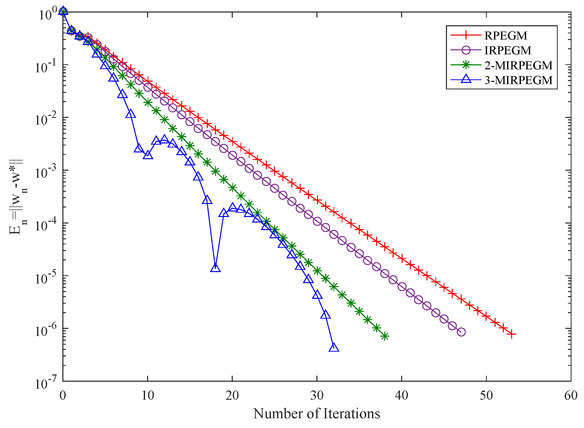
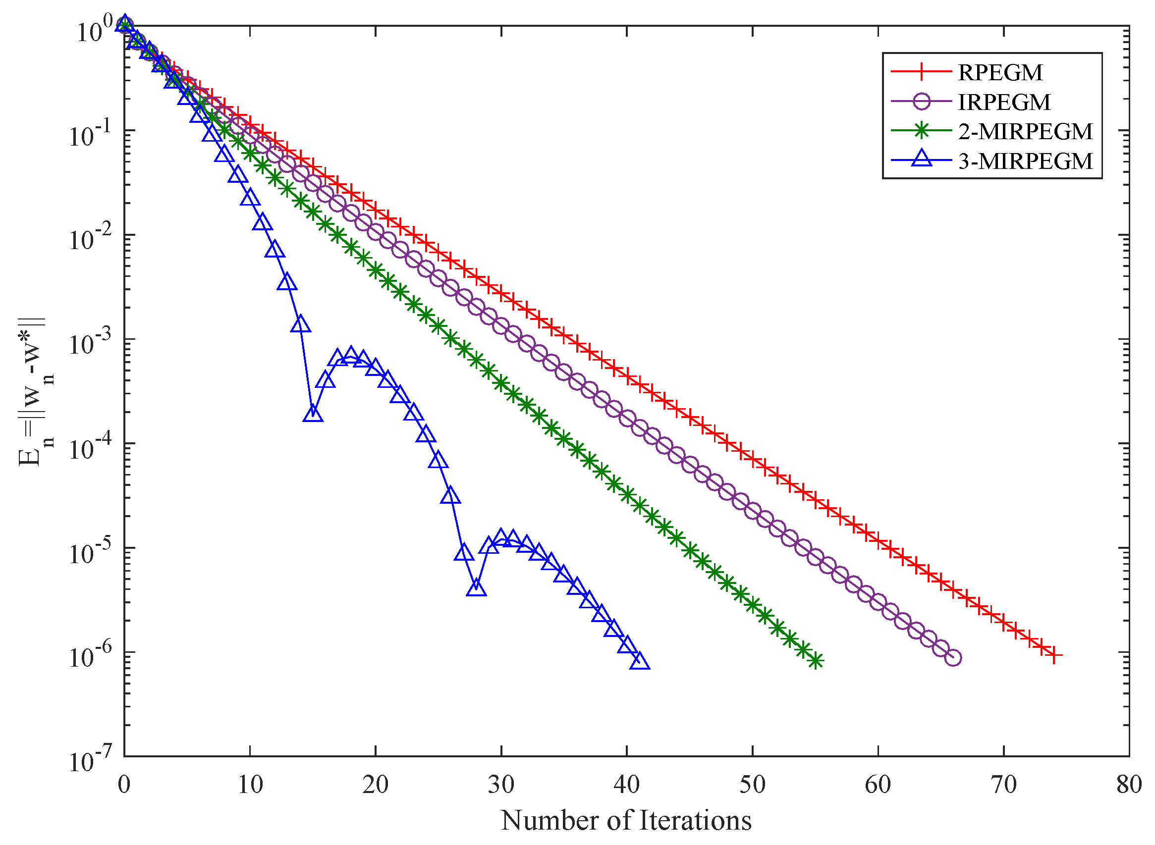
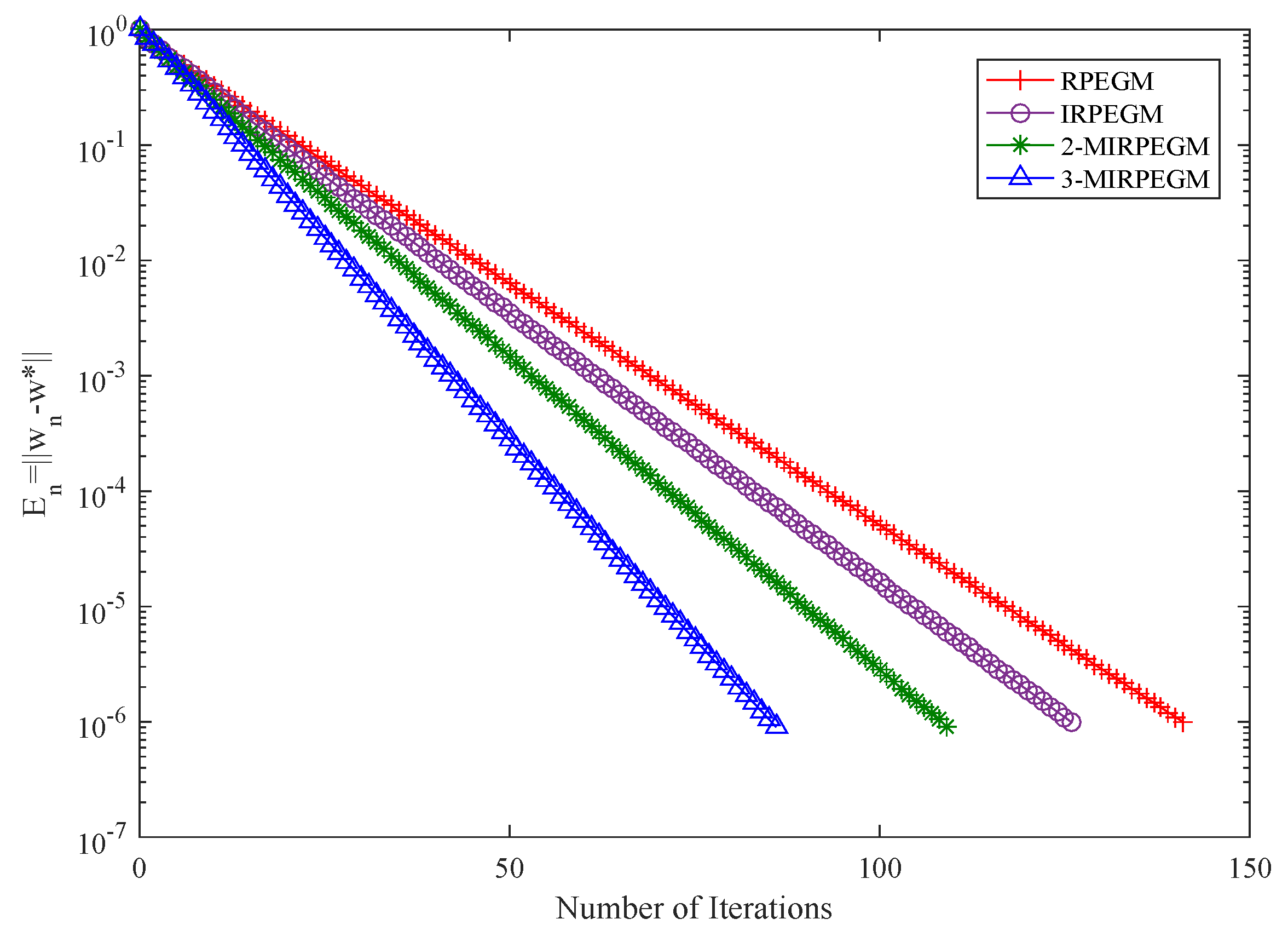
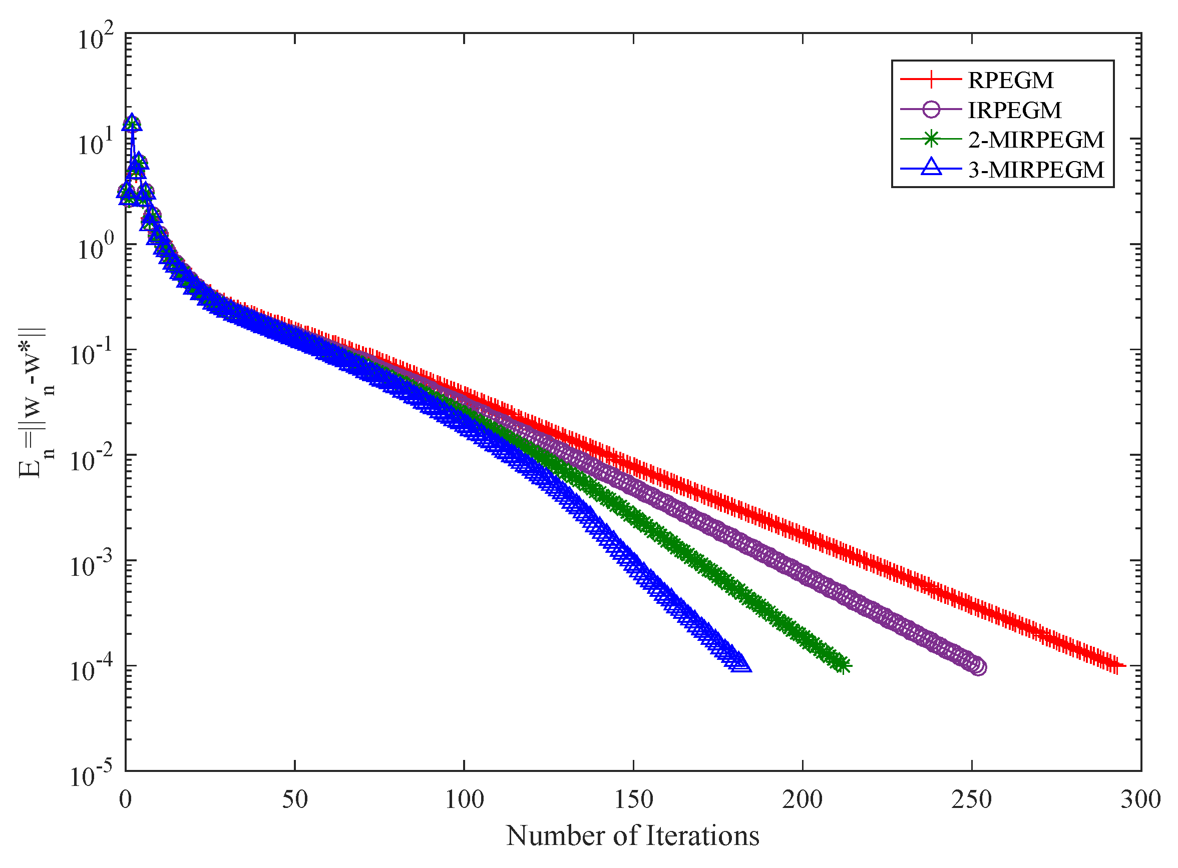
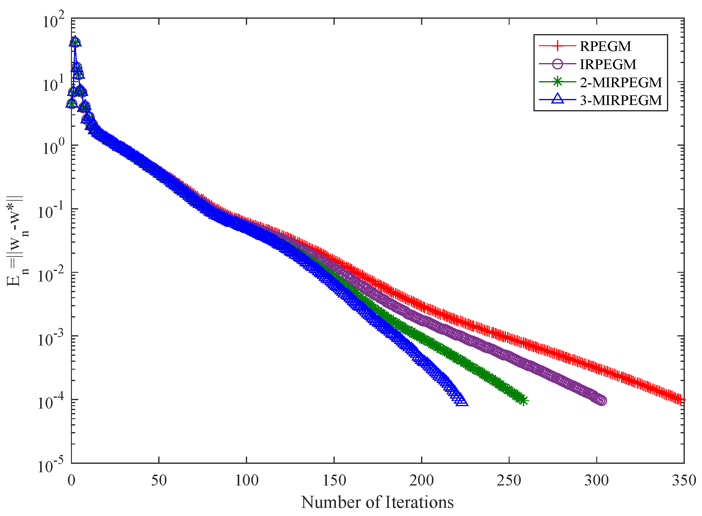
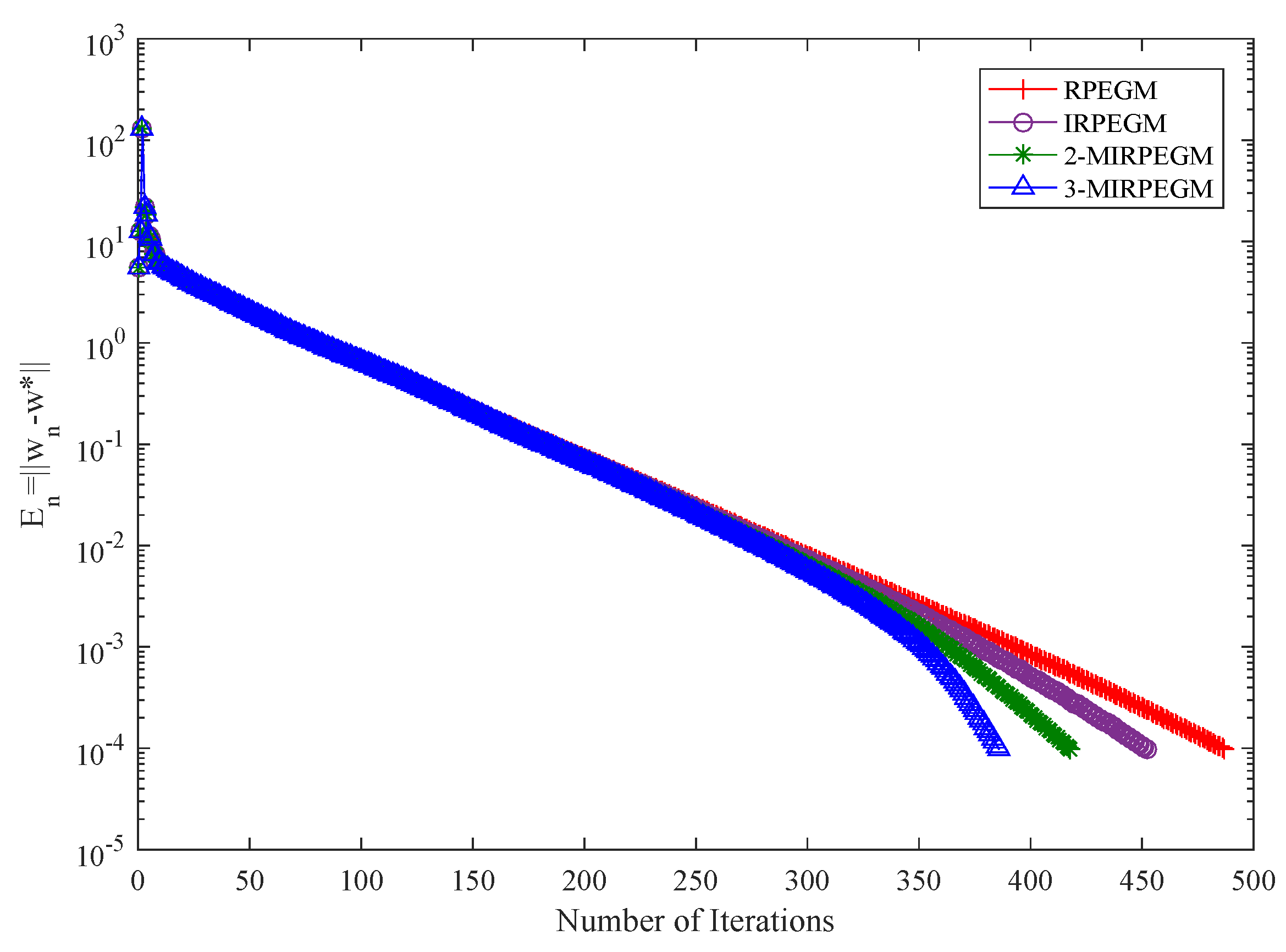
4. Numerical Examples

In the part, three numerical experiments are used to compare the effectiveness of our proposed algorithm. Through the analysis of results, it is not difficult to find that the efficiency of our algorithm proposed in our paper is higher. In the following three numerical experiments, we demonstrate the advantages of our proposed algorithms by studying the effects of one-step, two-step and three-step inertia on sequence convergence. All the procedures are compiled in Matlab 9.0 and executed on PC Desktop Intel(R) Core(TM) i5-1035G1 CPU @ 1.00 GHz 1.19 GHz, RAM 16.0 GB.

Example 2.

Let $\mathcal{C}=[-2,5]$. Denote mapping $A:\mathcal{H}\to \mathcal{H}$ as follows,

$$Aw=w+sinw,$$

for each $w\in \mathbb{R}$, where $\mathcal{H}=\mathbb{R}$. By the definition of A, we can show that the operator A is Lipschitzian and monotone. We use IRPEGM, 2-MIRPEGM and 3-MIRPEGM to denote the one-step, two-step and three-step inertia regularized Popov’s extra-gradient methods in this paper, respectively. For IRPEGM, 2-MIRPEGM and 3-MIRPEGM, we take $w_0=z_0=u_0=1$, ${\theta }_i=0.1$, ${\sigma }_{i,n}=\frac{1}{n^2}$; for RPEGM, we take $w_0=z_0=1$; and we take $\mu =0.3$, ${\alpha }_0=1$ and ${\alpha }_n={(n+1)}^{-\frac{3}{4}}$ for each method. Let $F=I$; through calculation, it is not difficult to deduce that $\mathrm{VI}(A,\mathcal{C})$= $\left\{0\right\}$. Therefore, HVIP (2) has one and only one solution: $w^{*}=0$. In this case, we set the algorithm to stop when $\parallel w_n-w^{*}\parallel \le {10}^{-6}$, and for each algorithm, we take ${\lambda }_0={\lambda }_1=$0.2, 0.1, and 0.05, respectively. The numerical experimental results are represented in Figure 1, Figure 2 and Figure 3.

It is not difficult to find from Figure 1, Figure 2 and Figure 3 that the number of steps required for sequence convergence in our IRPEGM, 2-MIRPEGM and 3-MIRPEGM is about 15%, 30%, and 40% less than that of RPEGM in [13], respectively. So, we can obtain that our algorithm is much broader, and much more efficient.

Example 3.

Let Q, K, and S∈${\mathbb{R}}^{s\times s}$, where K is symmetric matrices, and S is diagonal matrices with positive diagonal terms. We denote that $M=Q{Q}^{\mathrm{T}}+K+S$, then M is positive definite. Set mapping $A:{\mathbb{R}}^s\to {\mathbb{R}}^s$ to be defined as

$$Aw=Mw+p,$$

(20)

for each $w\in {\mathbb{R}}^s$, where $p\in {\mathbb{R}}^s$. Let $\mathcal{H}={\mathbb{R}}^s$, and set $\mathcal{C}$ to be defined as

$$\mathcal{C}=\{{(w^{\left(1\right)},w^{\left(2\right)},w^{\left(3\right)},\cdots ,w^{\left(s\right)})}^{\mathrm{T}}\in {\mathbb{R}}^s:-2\le w^{\left(j\right)}\le 5,j=1,2,\cdots ,s\}.$$

(21)

According to the definition of mapping A, it is obvious that operator A is Lipschitzian and monotone. Similarly, we use IRPEGM, 2-MIRPEGM, and 3-MIRPEGM to denote one-step, two-step and three-step inertia regularized Popov’s extra-gradient algorithm, respectively. For IRPEGM, 2-MIRPEGM, and 3-MIRPEGM, we take ${\sigma }_{i,n}=\frac{n}{-2}$, ${\theta }_i=0.2$, $w_0=z_0=u_0={(1,1,1,\cdots ,1)}^{\mathrm{T}}$ for RPEGM, and take $w_0=z_0={(1,1,1,\cdots ,1)}^{\mathrm{T}}$, $\mu =0.3$, ${\alpha }_0=1$, ${\alpha }_n={(n+1)}^{-\frac{3}{2}}$ for each method. Letting $F=I$, it is easy for us to obtain the solution set $\mathrm{VI}(A,\mathcal{C})=\left\{{(0,0,0,\cdots ,0)}^{\mathrm{T}}\right\}$; therefore, for HVIP (2), there is a unique solution $w^{*}$, and $w^{*}={(0,0,0,\cdots ,0)}^{\mathrm{T}}$. In this case, the algorithm stops when $\parallel w_n-w^{*}\parallel \le {10}^{-4}$, and we consider $s=10,20,30$, respectively. Throughout this experiment, $p={(0,0,\cdots ,0)}^{\mathrm{T}}$ and the diagonal term of D is stochastically and evenly created in (0,2), and all terms of Q and K are stochastically and equally created in (−2,2). Then, we get Figure 4, Figure 5 and Figure 6.

By looking at the features of Figure 4, Figure 5 and Figure 6, we can easily see that our algorithm has obvious advantages over RPEGM.

Example 4.

Set $\mathcal{H},\mathcal{C}$, and A as in Example 2. By definition of A, we can show that the operator A is Lipschitzian and monotone. We use IRPEGM to denote the one-step inertial regularized subgradient extra-gradient method, which is proposed by Jiang et al. [14]. For IRPEGM, IRSEGM, we take $w_0=z_0=u_0=1$, ${\theta }_1=0.1$, ${\sigma }_{i,n}=\frac{1}{n^2}$, ${\alpha }_0=1$, ${\alpha }_n={(n+1)}^{-\frac{3}{4}}$ for each method. Let

$$F\left(w\right)=\left\{\begin{array}{cc}w-1,\hfill & w<-1,\hfill \\ w-\sqrt{1-{(w+1)}^2},\hfill & -1\le w\le 0,\hfill \\ w+\sqrt{1-{(w-1)}^2},\hfill & 0\le w\le 1,\hfill \\ w+1,\hfill & w>1,\hfill \end{array}\right.$$

It is easy to verify that F is hemicontinuous, generalized Lipschitzian and strongly monotone on $\mathcal{H}$, but not Lipschitzian. Through calculation, it is not difficult to deduce that $\mathrm{VI}(A,\mathcal{C})$= $\left\{0\right\}$; therefore, HVIP (2) has one and only one solution $w^{*}=0$. In this case, we set that the algorithm stops when $\parallel w_n-w^{*}\parallel \le {10}^{-6}$. The numerical experiment results are represented in

Table 1. Numerical results of IRPEGM and IRSEGM as regards Example 4.

$\mathit{\mu }$	${\mathit{\lambda }}_1$	IRPEGM		IRSEGM
		Iter.	Time [s]	Iter.	Time [s]
0.2	0.2	128	0.9596	167	1.2030
	0.3	73	0.5893	99	0.8926
	0.4	73	0.5891	167	1.2683
0.3	0.2	76	0.6052	188	1.3341
	0.3	157	1.0814	184	1.3190
	0.4	76	0.6191	184	1.3587

.

5. Conclusions

In the paper, we propose a new multi-step inertial regularized generalized Popov’s extra-gradient method to solve the hierarchical variational inequality problem based on previous studies. Compared with previous algorithms, our algorithm has the following advantages. Firstly, compared with that of Hieu et al. [13], of the proposed algorithm, we introduce the multi-step inertial method to accelerate the convergence of the sequence. Secondly, we extend that F is Lipschitzian in [13] to hemicontinuous and generalized Lipschitzian; therefore, it is clear that our algorithm is relatively broader. Thirdly, compared with that of Jiang et al. [14], our algorithm only requires obtaining the value of $z_n$ under the action of A, with no need to discuss the behavior of $w_n$ under the action of A, and therefore, our algorithm is relatively simpler and more efficient.

References

1. Censor, Y.; Gibali, A.; Reich, S. The subgradient extragradient method for solving variational inequalities in Hilbert space. J. Optim. Theory Appl. 2011, 148, 318–335. [Google Scholar] [CrossRef] [PubMed] [Green Version]
2. Ceng, L.C.; Shehu, Y.; Wang, Y. Parallel Tseng’s extragradient mrthods for solving systoms of variational inequalities on hadamard manifolfs. Symmetry 2020, 12, 43. [Google Scholar] [CrossRef] [Green Version]
3. Hieu, D.V.; Strodiot, J.J.; Muu, L.D. An extragradient algorithm for solving variational inequalities. J. Optim. Theory Appl. 2020, 185, 476–503. [Google Scholar] [CrossRef]
4. Wang, Y.; Li, C.; Lu, L. A new algorithm for the common solutions of a generalized variational inequality system and a nonlinear operator equation in Banach spaces. Mathematics 2020, 8, 1994. [Google Scholar] [CrossRef]
5. Wang, Y.; Pan, C. Viscosity approximation methods for a general variational inequality system and fixed point problems in Banach spaces. Symmetry 2020, 12, 36. [Google Scholar] [CrossRef] [Green Version]
6. Yang, J.; Liu, H.; Li, G. Convergence of a subgradient extragradient algorithm for solving monotone variational inequalities. Numer. Algor. 2020, 84, 389–405. [Google Scholar] [CrossRef]
7. Reich, S.; Thong, D.V.; Cholamjiak, P.; Long, L.V. Inertial projection-type methods for solving pseudomonotone variatinal inequality problems in Hilbert spaces. Numer. Algor. 2021, 88, 813–835. [Google Scholar] [CrossRef]
8. Thong, D.V.; Shehu, Y.; Iyiola, O.S.; Thang, H.V. New hybrid projection methods for variational inequalities involving pseudomonotone mappings. Optim. Eng. 2021, 22, 363–386. [Google Scholar] [CrossRef]
9. Korpelevich, G.M. An extragradient method for finding saddle points and for other problems. Ekon. Mat. Metod. 1976, 12, 747–756. [Google Scholar]
10. Popov, L.D. A modification of the Arrow-Hurwicz method for searching for saddle points. Mat. Zameki. 1980, 28, 777–784. [Google Scholar]
11. Malitsky, Y.V.; Semenov, V.V. An extragradient algorithm for monotone variational inequalities. Cybern. Syst. Anal. 2014, 50, 271–277. [Google Scholar] [CrossRef]
12. Hieu, D.V.; Anh, P.K.; Muu, L.D. Modified extragradient-like algorithms with new stepsizes for variational inequalities. Comput. Optim. Appl. 2019, 73, 913–932. [Google Scholar] [CrossRef]
13. Hieu, D.V.; Moudafi, A. Regularization projection method for solving bilevel variational inequality problem. Optim. Lett. 2020, 15, 205–229. [Google Scholar] [CrossRef]
14. Jiang, B.; Wang, Y.; Yao, J.C. Multi-step inertial regularized methods for hierarchical variational inequality problems involving generalized lipschitz continuous and hemicontinuous mappings. Mathematics 2021, 9, 2103. [Google Scholar] [CrossRef]
15. Hammad, H.A.; Renman, H.; Almusawa, H. Tikhonov regularization terms for Accelerating inertial mann-like algorithm with applications. Symmetry 2021, 13, 554. [Google Scholar] [CrossRef]
16. Zhou, H.; Zhou, Y.; Feng, G. Iterative methods for solving a class of monotone variational inequality problems with applications. J. Inequal. Appl. 2015, 2015, 68. [Google Scholar] [CrossRef] [Green Version]
17. Xu, H.K. Averaged mappings and the gradient-projection algorithm. J. Optim. Theory Appl. 2011, 150, 360–378. [Google Scholar] [CrossRef]
18. Yang, J.; Liu, H. Strong convergence result for solving monotone variational inequlities in Hilbert space. Numer. Algor. 2019, 80, 741–752. [Google Scholar] [CrossRef]
19. Kraikaew, R.; Saejung, S. Strong convergence of the Halpern subgradient extragradient method for solving variational inequalities in Hilbert spaces. J. Optim. Theory Appl. 2014, 163, 399–412. [Google Scholar] [CrossRef]
Figure 1. Comparison of RPEGM, IRPEGM, 2-MIRPEGM and 3-MIRPEGM in Example 2 with λ 1 = 0.2 .
Symmetry 14 00187 g001
Figure 2. Comparison of RPEGM, IRPEGM, 2-MIRPEGM and 3-MIRPEGM in Example 2 with λ 1 = 0.1 .
Symmetry 14 00187 g002
Figure 3. Comparison of RPEGM, IRPEGM, 2-MIRPEGM and 3-MIRPEGM in Example 2 with λ 1 = 0.05 .
Symmetry 14 00187 g003
Figure 4. Comparison of RPEGM, IRPEGM, 2-MIRPEGM and 3-MIRPEGM in Example 3 with s = 10 .
Symmetry 14 00187 g004
Figure 5. Comparison of RPEGM, IRPEGM, 2-MIRPEGM and 3-MIRPEGM in Example 3 with s = 20 .
Symmetry 14 00187 g005
Figure 6. Comparison of RPEGM, IRPEGM, 2-MIRPEGM and 3-MIRPEGM in Example 3 with s = 30 .
Symmetry 14 00187 g006