Abstract
In order to deal with the fast, large-angle attitude maneuver with flexible appendages, a finite-time attitude controller is proposed in this paper. The finite-time sliding mode is constructed by implementing the dynamic sliding mode method; the sliding mode parameter is constructed to be time-varying; hence, the system could have a better convergence rate. The updated law of the sliding mode parameter is designed, and the performance of the standard sliding mode is largely improved; meanwhile, the inherent robustness could be maintained. In order to ensure the system’s state could converge along the proposed sliding mode, a finite-time controller is designed, and an auxiliary term is designed to deal with the torque caused by flexible vibration; hence, the vibration caused by flexible appendages could be suppressed. System stability is analyzed by the Lyapunov method, and the superiority of the proposed controller is demonstrated by numerical simulation.
1. Introduction
Current space missions, such as push-broom imaging and stare imaging, need satellites that have the ability to perform fast large-angle maneuvers. However, standard controllers, such as the PID controller and the sliding mode controller, have the issue of a low convergence rate. It is necessary to develop an attitude controller with a faster convergence rate. Furthermore, the deformation and vibration of flexible appendages would bring unexpected torque on the satellite system; hence, the overall goal of this paper is to develop a satellite attitude controller subject to fast large-angle attitude maneuvers with a better convergence rate compared to standard controllers. Meanwhile, the flexible vibrations could be suppressed.
In the field of satellite attitude control, PID control and sliding mode control are the most mature and widely used methods. They both have the advantage of simple structures and strong robustness; hence, a lot of work has been performed by researchers. However, a low convergence rate is the main drawback of these two methods. Li [1,2,3] developed PID controllers for satellite’s fast maneuvering with flexible appendages, and standard PID controllers are modified in his work. Hence, the system could have a better convergence rate. There is also some work [4,5] focusing on satellite orbit control, and the main goal of these two papers is to optimize energy consumption. The sliding mode controller is also a mature method in the field of satellite attitude control. Chakrabarti [6] and Ye [7] designed sliding mode controllers for satellite attitude maneuvers; the standard sliding mode for satellite attitude control is modified in these works, and the system robustness is enhanced. However, the system convergence rate is not taken into consideration in these works. In order to improve the system convergence rate, Li [8,9] has done some work, and the standard sliding mode is modified by Bang-Bang logic and dynamic sliding mode. The system convergence rate is largely improved by implementing the updated law of the sliding mode parameter. Moreover, Xiao [10,11,12] has performed some work focusing on the modification of sliding mode controllers. The controllers with fault-tolerant and strong robustness are proposed in these works. Ye [13] also designed a sliding mode control algorithm for an attitude tracking controller, and his main focus is the system convergence rate. In his work, it is pointed out that by optimizing the trajectory of angular velocity, the system could have both a fast convergence rate and low energy consumption. However, the common drawback of these works is that the system convergence rate is exponential, which means the system state would reach its equilibrium point with infinite time. The terminal convergence rate is relatively low in these works, and it is necessary to develop a controller with a better convergence rate, especially for fast attitude maneuverable conditions.
In order to deal with the exponential convergence rate issue, finite-time control theory, which could largely improve the system convergence rate to near its equilibrium point, is developed by researchers. Li [14] developed a finite-time controller with three stage structures, and a braking curve for angular velocity is constructed. The system convergence rate is improved by maintaining angular velocity revers to attitude quaternion; meanwhile, its norm is reaching its upper bound for as long as possible. The singularity issue is solved by using the property when the angular velocity is reversed to the vector of the Euler Axis. Liang [15,16], Wang [17,18] and Wu [19,20] also designed finite-time controllers for satellite attitude control, and their main focus is the structure of the finite-time sliding mode. It is pointed out that the key to achieving finite-time stability is to construct the fraction order of the system state properly. However, these works do not consider the flexible deformation of large flexible appendages, such as solar sails and large antennas, which are very common in satellites. Noting that when a satellite is on a fast attitude maneuver, the flexible vibrations can not be ignored; hence, it is necessary to design controllers that are robust to flexible deformations.
In order to deal with the satellite attitude control issue considering flexible vibration, some fundamental work [21,22,23,24] has been done. Wie constructed the basic structure of a PID controller for satellite attitude control and some typical methods for stability analysis is proposed. Some typical sliding mode surfaces are also proposed for satellite attitude control. Generally, the basic idea to deal with flexible vibrations could be concluded as following two aspects: 1. treat it as another kind of disturbance with a normal upper bound; 2. design a state observer to estimate it based on its dynamic model. The former is easier for engineering practice, and the latter has better performance in theoretical research.
In this paper, a finite-time controller for a satellite capable of fast, large-angle maneuvers with flexible appendages will be proposed. The next section will give the dynamic and kinetic models used in this paper, Section 3 is the core of this paper, and the finite-time controller will be given in this section. Section 4 will demonstrate the performance by numerical simulation, and Section 5 will conclude this paper.
2. Explanation of the Symbols Used in This Paper
In order to make it easier to understand this paper, the symbols used in this paper are explained in the following Table 1.

Table 1.
Explanation of the symbols.
3. Dynamic and Kinetic Model
The dynamic model of the rigid satellite could be written as follows.
where is the angular velocity, is the inertia matrix of satellite, which is a symmetric matrix, is the unknown disturbance torque with a normal upper bound . is the coupling matrix between the flexible appendages and the rigid body and describes how the flexible appendages influence the rigid body, is the modal coordinate vector, its definition could be found in Table 1, and are defined as follows.
where is the natural frequency and is the associated damping, and is the number of the elastic modes need to be considered.
Product matrix of vector is defined as:
Generally, the inertia matrix could not be accurately known, and it is assumed that:
where is the inertia matrix best estimate and is the error matrix. Product matrix has an important property, which will be used in the latter part that the eigenvalues of satisfies:
Define and as follows.
The dynamic model (1) could be transformed to:
where are defined as follows.
The kinetic model based on attitude quaternion could be written as follows.
where and the eigenvalue of satisfies:
In order to simplify the text, the maximum and minimum eigenvalue of matrix is described as and .
Considering that and describes the same attitude, it is assumed that in this paper.
Furthermore, it is worth noticing that in engineering practice, system angular velocity and control torque has its norm upper bound, and it is assumed to be and in this paper.
4. Finite-Time Controller
4.1. Problem Description
The sliding mode control method has been proposed for a decade, and a lot of work based on this method has been performed on the satellite attitude control issue. The most widely used and standard sliding mode for satellite attitude control could be written as follows.
After reaching this sliding mode surface, the system state has such properties:
When the system maneuvers along (11), the angular velocity vector is reversed to the attitude quaternion vector, and a lot of work has been done based on this sliding mode. The model uncertainty and unknown disturbance issue could be effectively solved using sliding mode (11), and it could be concluded that the reverse property could improve system robustness. However, based on Equation (11), it could be easily found that the convergence rate of is exponential, which means the system would reach the equilibrium point with infinite time and the convergence rate needs to be improved.
In order to improve the system convergence rate, a finite-time controller is an effective method. Generally, in order to achieve the finite-time stability, a fraction order feedback is used as follows to construct the sliding mode.
Sliding mode (13) would bring another issue, i.e., the singularity issue. Since the control torque is always related to , i.e., the second derivative of , the singularity term would be brought into the controller. In order to deal with the singularity issue, some typical finite-time controllers are designed [14]. However, the system robustness issue is not taken into consideration, and the reverse property does not hold in these works. System robustness needs to be improved to suppress the perturbations, such as inertia matrix uncertainty and unknown disturbance. In summary, the robustness issue and singularity issue should be both taken into consideration to design the robust finite-time controller.
Based on the discussion above, the goal of this paper could be: design a finite-time controller for satellite stabilization issues and the following properties should be satisfied:
- Compared with the standard sliding mode, the system convergence rate near the equilibrium point should be largely improved;
- Finite-time stability should be satisfied, i.e., there exist positive scalar and to satisfy following inequality;
- The singularity issue should be solved, i.e., are all bound during the whole control process;
- The controller should be robust to inertia matrix uncertainty and unknown disturbance torque.
4.2. Finite-Time Sliding Mode
In paper [9], the author pointed out that the fixed sliding mode caused the low convergence rate, and a dynamic sliding mode is constructed in this paper. The maneuver stage with constant angular velocity and converge stage with constant angular acceleration are designed based on the updated law of sliding mode parameter , and the system convergence rate is largely improved compared to the standard sliding mode. Inspired by the method in [3], the finite-time sliding mode proposed in this paper could be written as follows.
where the initial value of satisfies , is a small positive scalar, and are all positive scalars.
A sliding mode (15) has the same structure as a standard sliding mode; hence. the reversed property could be maintained. Moreover, the same structure could make it possible to design a robust finite-time controller based on standard sliding mode methods. Based on (15), it could be found that the maneuvering process is constructed in two stages: in the first stage, i.e., , the system performance is totally the same as that of a standard sliding mode, and the sliding mode parameter is fixed; in the second stage, i.e., , it could be treated as a system that has reached the sliding mode, and angular velocity vector has been reversed to the attitude quaternion vector. In this stage, the sliding mode parameter begins to update. Moreover, based on the updated law of , it could be found that is monotonically increasing to affect the exponential convergence rate. The key work of this paper is the updated law of the sliding mode parameter and when the system convergences along (15), i.e., , system (5) would converge to its equilibrium point within finite-time, and during this process, and are all norm upper bound.
The next step is to discuss the finite-time stability of the sliding mode (15). When the system reaches the sliding mode (15), it is defined as follows, and its derivative could be calculated as:
In order to achieve the goal of finite-time stability, the derivative of Lyapunov function should satisfy the following inequality:
Compared with (14) and (15), it could be that if there exists a positive scalar to satisfy the following inequality, the finite-time stability could be ensured.
In order to satisfy the finite-time condition (20), the fixed parameter is not feasible since the right part of (20) tends towards infinite, and a very large would cause the control torque of an angular velocity to exceed the system upper bound drastically. Hence, it is necessary to design a time-variable parameter and its update law to satisfy (20), and that is how the dynamic sliding mode (15) is found. In fact, selecting parameters as follows, it could be found that:
Noting that the structure of the sliding mode parameter update law in (15), it could be found that:
Based on (21) and (22), it could be found that finite-time condition (20) is satisfied, and (19) could be transformed to:
The system converge time satisfies:
The next step is to improve on sliding mode (15), are all norm upper bound. It is obvious that angular velocity satisfies following the property and is the norm upper bound.
Calculating the derivative of angular velocity, it could be found that:
where is the unit direction vector of attitude quaternion, which is defined as . Noting that , hence, are all norm upper bound during the whole maneuver process, and the demand control torque is also the norm upper bound, i.e., the singularity issue is solved. However, it is also worth noticing that on sliding mode (15), the system parameter tends towards infinite since is not the norm upper bound. In order to avoid this situation, we rewrite the sliding mode as follows.
where and are all small positive scalars. The difference between sliding mode (15) and (27) is simple when the system approaches the equilibrium point, the sliding mode parameter stops updating, and the singularity issue of could be solved, and the system state could converge to the field of within finite-time, hence, if a small enough parameter is selected (in fact, considering the disturbance system could not reach the absolute equilibrium point, hence reaching the field near system equilibrium could be treated as reaching equilibrium point), the systems finite-time stability could be ensured, and this property will be proven in next section.
4.3. Finite-Time Controller
After the finite-time sliding mode surface is derived, the next step is to construct a finite-time controller to ensure the system state could converge to the proposed sliding mode surface within finite time and could converge to its equilibrium point along this sliding mode surface. Furthermore, the proposed controller could resist the disturbance torque caused by flexible appendages.
where is a positive scalar, is a positive scalar which satisfies , is the sign function of vector , vector function and is defined as follows:
where is a positive scalar which satisfies with as the maximum eigenvalue value of the error inertia matrix . Furthermore, in (30) is a positive scalar, which is meant to resist the disturbance torque caused by flexible appendages, and the method to select this parameter will be given in a later text.
The next step is to discuss the system stability governed by the controller (28). We select the Lyapunov function as follows
It is obvious that Function (31) is a semi-positive definite when and only when Function (31) equals zero. Except for the condition that , we calculate the derivative of (31) and the substitute controller (28), and it could be found that:
Similarly, we calculate the derivative of Lyapunov function at the stage of , it could be found that:
Noting the definition of and in (30), it could be easily found that the last two terms in (32) and (33) are negative definites, i.e.,:
Hence (32) and (33) could be transformed to:
It is obvious the first term in (35) satisfies the finite-time stability condition, and if the last term in (35) is a negative definite, the system could converge to the designed sliding mode surface within a finite time. Moreover, it could be found that the term that needs to be suppressed is the flexible vibration; although, its modal state is hard to get by sensors on satellite, its dynamic model is known; hence, the modal state could be estimated by a state observer. We define and its update law as follows.
where:
It could easily be found that the estimation variable has the same dynamic model as the modal state . We define the estimation error variable as follows.
Substitute models (1) and (36) into (38), and it could be found that:
Obviously, the only differences are the terms and caused by model uncertainty and disturbance torque. Noting that and are both positive definite matrices, the error variable is typical of the Lagrange system and would track by an exponential rate. Furthermore, noting that is a relatively small term, it could be treated that estimation variable could track modal state , but there exists a small tracking error. Hence, the auxiliary term could be defined as follows.
The function of the last term, , is to offset the effect caused by the model error . Noting the ith modal estimation error could be described as:
The analytical solution of (41) could be written as follows.
Noting that is a relatively small term, the major part is the transient term, i.e., the second term in (42)–(44). The idea to offset the transient term is to design ’s envelop function, as Figure 1 shows.
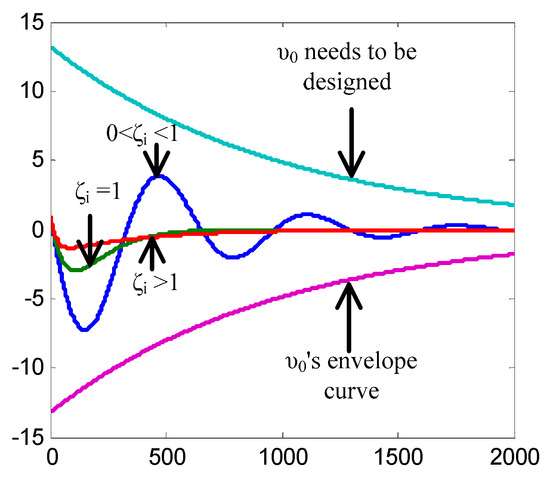
Figure 1.
Envelop function.
The basic idea to design is to ensure its norm is larger than the norm of , and noting Equations (42)–(44), could be designed as follows.
By selecting the initial value of (in this paper, is selected five times larger than the model error and is selected 1/5 times less than the minimum value of ), it could be found that:
Hence, the derivative of in (35) satisfies:
Hence, the sliding mode state could converge to zero within finite time, and based on the previous discussion, the system state could converge to the field near the equilibrium point within finite timem and the systems finite-time stability has been proven.
Moreover, it could be found that the sign function terms in (40) and (28) (except the disturbance term ) tend to zero as the system converges to its equilibrium point and would not cause high-frequency vibrations.
5. Simulation
Comparing Group
Set the system parameters as follows.
Set the disturbance as Gauss white noise and its norm upper bound as follows.
Group A
In order to demonstrate the superiority of the controller in this paper, the standard sliding mode controller (50) is compared.
Select the control parameters as follows.
The simulation results of the standard sliding mode controller (50) are given as follows. Based on Figure 2 and Figure 3, it could be found that the system convergence time is more than 300 s, and the steady accuracy of angular velocity and attitude quaternion is about and . A system governed by a standard sliding mode controller could converge to its equilibrium point, but the convergence rate is relatively slow. Furthermore, based on Figure 4, it could also be found that the modal state also converges to zero as the angular velocity converges to zero, and the maximum vibration is about 0.1 according to numerical simulation.
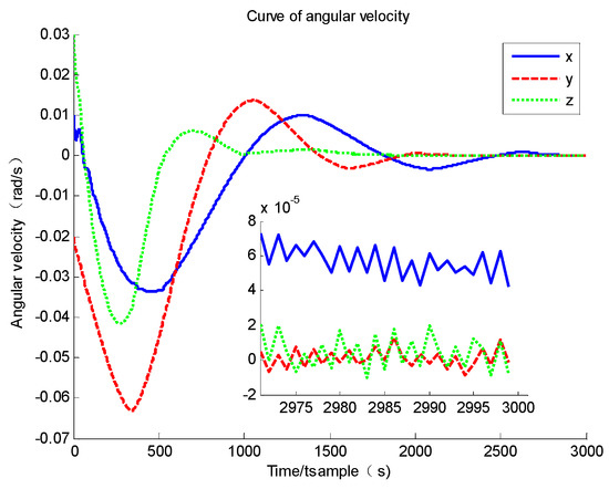
Figure 2.
Curve of angular velocity.
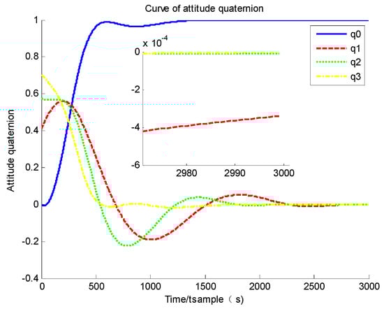
Figure 3.
Curve of attitude quaternion.
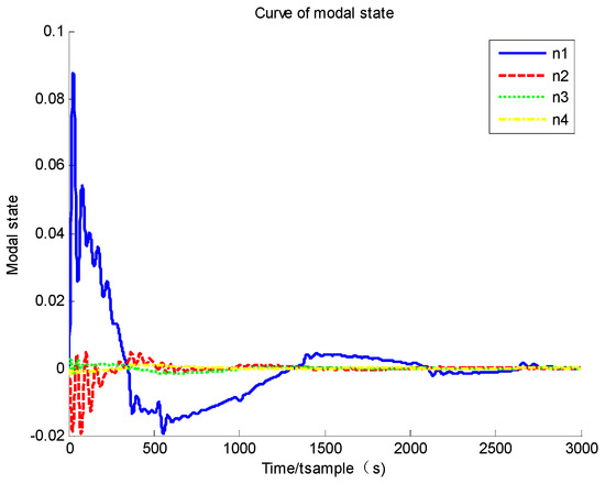
Figure 4.
Curve of modal state.
Group B
The next step is to demonstrate the performance of the finite-time controller proposed by Li [14] in 2017. In this paper, the author pointed out that by designing the trajectory of angular velocity properly, the system convergence rate could be largely improved compared to a standard sliding mode controller. Moreover, finite-time stability, as discussed in this paper, is proven in Li’s work; hence, this method is compared with the method proposed in this paper. The finite-time controller proposed in Li’s work could be written as Equation (52) and select controller parameters as Equation (53) [14].
The simulation results of the finite-time controller (52) are given as follows.
Based on Figure 5 and Figure 6, it could be found that the system converges to its equilibrium point and the convergence time is about 100 s, which is largely improved compared to a standard sliding mode controller. Furthermore, based on Figure 5 and Figure 6, it could be found that the system accuracy at the steady stage is about and of angular velocity and attitude quaternion, which is also improved compared to Group A. The only drawback of this controller is the flexible deformation. Based on Figure 7, although a modal state could converge to zero along the converge of angular velocity, the maximum modal state is about 0.35, and its frequency is also much higher than that of Group A. The high-frequency vibration causes system state chattering near its equilibrium point (based on Figure 5, three axes of angular velocity all have a chattering issue).
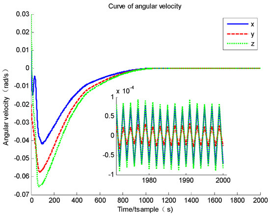
Figure 5.
Curve of angular velocity.
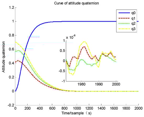
Figure 6.
Curve of attitude quaternion.
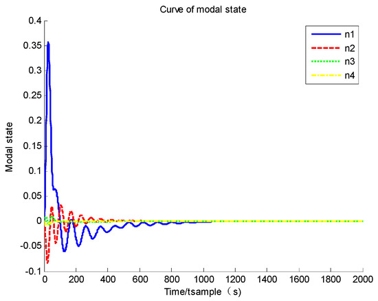
Figure 7.
Curve of modal state.
Group C
The PID control algorithm is also a mature and widely used method in satellite attitude control, and the set control parameters are as follows.
The system performance is governed by PID controllers and are shown as follows.
Based on Figure 8 and Figure 9, it could be found that the system governed by a PID controller is stable, and the convergence time is about 200 s, which is slower than the standard sliding mode controller, but the structure is the strongest and most robust. It could be easily found that the shock of the system state near its equilibrium point is much relieved. Moreover, based on Figure 10, it could be found that the PID controller could also suppress the flexible vibration.
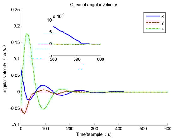
Figure 8.
Curve of angular velocity.
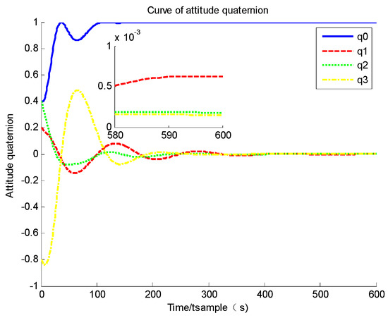
Figure 9.
Curve of attitude quaternion.
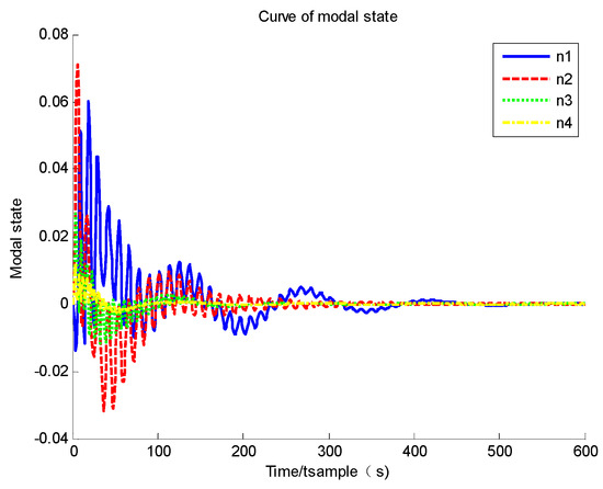
Figure 10.
Curve of modal state.
Group D
The final step is to demonstrate the performance of the controller proposed in this paper. We selected the control parameters as follows.
Moreover, we assume the initial modal state estimation error as follows.
We selected the auxiliary term as follows.
Generally, the larger parameter and could bring a better system convergence rate; however, the system control torque and angular velocity is increased. The parameter determines the rate the system converges to the desired sliding mode. The parameter determines the suppression for the estimation error; when the initial estimation error, disturbance and model error are relatively large, this parameter should be selected to be larger.
The simulation results are given as follows. Based on Figure 11 and Figure 12, it could be found that the system converges to its equilibrium point and the convergence time is about 45 s, which is the fastest of the three groups, and the system accuracy at a steady stage is and of angular velocity and attitude quaternion, which is also the best in the three groups. Moreover, it could be found that the initial value of the sliding mode parameter is 1/3 of Group A, but the system convergence time is about 1/8. This proves that by enlarging the sliding mode parameter, the system convergence time could be largely improved. Based on Figure 13, it could be found that the modal state converges to zero, and its maximum value is about 0.2, which is largely improved compared to the finite-time controller in Group B. Comparing the simulation results of Group D with Groups A, B and C, it could be found that the upper bound and frequency of flexible vibration is suppressed. Hence, the chattering issue is largely relieved (seen in Figure 11, the shocking of angular velocity only exists on the Z-axis and its frequency is much lower). Based on Figure 14, it could be found that although there exists la arge initial estimation error, the state observer could also track the real modal state, and the estimation error tends to zero. Based on Figure 15, it could be found that the sliding mode parameter stops updating when the system state nears its equilibrium point; hence, the system does not have a singularity issue.
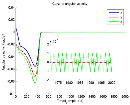
Figure 11.
Curve of angular velocity.
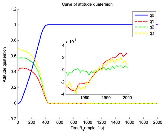
Figure 12.
Curve of attitude quaternion.
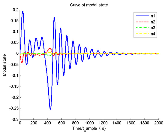
Figure 13.
Curve of modal state.
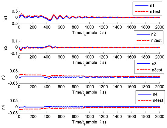
Figure 14.
Curve of modal state and its estimation.
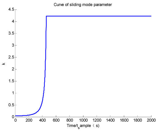
Figure 15.
Curve of sliding mode parameter.
The performance of the three groups of controllers is summarized in the following Table 2.
Table 2.
Comparison of the three controllers.
Based on the comparison in Table 2, it could be found that the major advantages of the method proposed in this paper are its convergence rate, steady accuracy and none singularity issue. Although the updated law of the sliding mode parameter would cause relatively large flexible vibration, the modal state estimation algorithm and auxiliary term could relieve the effect.
6. Conclusions
In this paper: a finite-time controller based on the dynamic sliding mode is proposed, and the system convergence rate is largely improved compared to the standard sliding mode and existing finite-time controller. It is proven that by implementing the updated law of the sliding mode parameter, the system could converge to the field near the equilibrium point within finite time, without causing the singularity issue during the whole control process. Furthermore, it is proven that the key to improving the system performance is to design an angular velocity trajectory properly, and the method proposed in this paper is the updated law of the sliding mode parameter; by implementing this method, the drawback of dropping too fast of angular velocity is avoided. Moreover, a state observer is designed for flexible vibration, and an auxiliary term, which is converging slower than the system state, is designed to suppress the effect of the estimation error. The simulation results prove the effectiveness of the method proposed in this paper, and future work could focus on the modification of the sign function in controllers to avoid high-frequency vibration near the system’s equilibrium point.
Author Contributions
Conceptualization, Y.L. and H.L.; methodology, Y.L. and L.X.; software, Y.L. and L.X.; validation, Y.L.; formal analysis, Y.L.; investigation, H.L.; resources, L.X.; data curation, L.X.; writing—original draft preparation, Y.L.; writing—review and editing, Y.L. All authors have read and agreed to the published version of the manuscript.
Funding
This research was funded byNational Natural Science Foundation of China, grant number 61903289, 62003375 and 6210345.
Institutional Review Board Statement
Not applicable.
Informed Consent Statement
Not applicable.
Data Availability Statement
If anyone wants to get the original data of this paper, please contact liyou@xidian.edu.cn.
Acknowledgments
This work was supported partially by the National Natural Science Foundation of China (Project Nos. 61903289, 62003375 and 62103452). The authors greatly appreciate the above financial support. The authors would also like to thank the associate editor and reviewers for their valuable comments and constructive suggestions that helped to improve the paper significantly.
Conflicts of Interest
The authors declare that we have no financial and personal relationships with other people or organizations that can inappropriately influence our work, there is no professional or other personal interest of any nature or kind in any product, service and/or company that could be construed as influencing the position presented in, or the review of, the manuscript entitled.
References
- Gao, S.; Li, Y.; Yao, S.Y. Robust PD+ Control Algorithm for Satellite Attitude Tracking for Dynamic Targets. Mathematical Problems in Engineering. Math. Probl. Eng. 2021, 2021, 6680994. [Google Scholar]
- Li, Y.; Ye, D. Robust PID controller for flexible satellite attitude control under angular velocity and control torque constraint. Asian J. Control 2020, 22, 1327–1344. [Google Scholar] [CrossRef]
- Li, Y.; Sun, Z.W.; Ye, D. Time Efficient Robust PID Plus Controller for Satellite Attitude Stabilization Control Considering Angular Velocity and Control Torque Constraint. J. Aerosp. Eng. 2017, 30, 04017030. [Google Scholar] [CrossRef]
- Xu, Y.; Lu, Z.; Shan, X.; Jia, W.; Wei, B.; Wang, Y. Study on an Automatic Parking Method Based on the Sliding Mode Variable Structure and Fuzzy Logical Control. Symmetry 2018, 10, 523. [Google Scholar] [CrossRef] [Green Version]
- Zhang, Y.; Nie, Y.; Chen, L. Adaptive Fuzzy Fault-Tolerant Control against Time-Varying Faults via a New Sliding Mode Observer Method. Symmetry 2021, 13, 1615. [Google Scholar] [CrossRef]
- Chakrabarti, D.; Selvaganesan, N. PD and PD beta based sliding mode control algorithms with modified reaching law for satellite attitude maneuver. Adv. Space Res. 2020, 65, 1279–1295. [Google Scholar] [CrossRef]
- Ye, D.; Zhang, H.Z.; Tian, Y.X.; Zhao, Y.; Sun, Z.W. Fuzzy Sliding Mode Control of Nonparallel-ground-track Imaging Satellite with High Precision. Int. J. Control. Autom. Syst. 2020, 18, 1617–1628. [Google Scholar] [CrossRef]
- Gao, S.; Li, Y.; Xue, H.F.; Yao, S.Y. Dynamic Sliding Mode Controller with Variable Structure for Fast Satellite Attitude Maneuver. Math. Probl. Eng. 2021, 2021, 5539717. [Google Scholar]
- Li, Y.; Ye, D.; Sun, Z.W. Time efficient sliding mode controller based on Bang-Bang logic for satellite attitude control. Aerosp. Sci. Technol. 2018, 75, 342–352. [Google Scholar] [CrossRef]
- Xiao, B.; Yin, S.; Wu, L.G. A structure simple controller for satellite attitude tracking maneuver. IEEE Trans. Ind. Electron. 2017, 64, 1436–1446. [Google Scholar] [CrossRef]
- Xiao, B.; Yin, S.; Gao, H.J. Tracking control of robotic manipulators with uncertain kinematics and dynamics. IEEE Trans. Ind. Electron. 2016, 63, 6439–6449. [Google Scholar] [CrossRef]
- Hu, Q.L.; Zhang, Y.M.; Huo, X.; Xiao, B. Adaptive integral-type sliding mode control for spacecraft attitude maneuvering under actuator stuck failures. Chin. J. Aeronaut. 2011, 24, 32–45. [Google Scholar] [CrossRef] [Green Version]
- Ye, D.; Zou, A.M.; Sun, Z.W. Predefined-Time Predefined-Bounded Attitude Tracking Control for Rigid Spacecraft. IEEE Trans. Aerosp. Electron. Syst. 2021. [Google Scholar] [CrossRef]
- Li, Y.; Ye, D.; Sun, Z.W. Robust finite time control algorithm for satellite attitude control. Aerosp. Sci. Technol. 2017, 68, 46–57. [Google Scholar] [CrossRef]
- Liang, H.Z.; Wang, J.Y.; Sun, Z.W. Robust decentralized coordinated attitude control of spacecraft formation. Acta Astronaut. 2011, 69, 280–288. [Google Scholar] [CrossRef]
- Liang, H.Z.; Sun, Z.W.; Wang, J.Y. Finite-time attitude synchronization controllers design for spacecraft formations via behavior-based approach. Part G J. Aerosp. Eng. 2013, 227, 1737–1753. [Google Scholar] [CrossRef]
- Wang, J.Y.; Liang, H.Z.; Sun, Z.W. Dual-quaternion-based finite-time control for spacecraft tracking in six degrees of freedom. J. Aerosp. Eng. 2013, 227, 528–545. [Google Scholar] [CrossRef]
- Wang, J.Y.; Liang, H.Z.; Sun, Z.W.; Zhang, S.J.; Liu, M. Finite-time control for spacecraft formation with dual-number-based description. J. Guid. Control. Dyn. 2012, 35, 950–962. [Google Scholar] [CrossRef]
- Wu, S.N.; Wang, R.; Radice, G.; Wu, Z.G. Robust attitude maneuver control of spacecraft with reaction wheel low-speed friction compensation. Aerosp. Sci. Technol. 2015, 43, 213–218. [Google Scholar] [CrossRef]
- Wu, S.N.; Radice, G.; Sun, Z.W. Robust finite-time control for flexible spacecraft attitude maneuver. J. Aerosp. Eng. 2014, 27, 185–190. [Google Scholar] [CrossRef]
- Wie, B.; Barba, P.M. Quaternion Feedback for Spacecraft Large Angle Maneuvers. J. Guid. Control. Dyn. 1985, 8, 360–365. [Google Scholar] [CrossRef]
- Wie, B.; Weiss, H.; Arapostathis, A. Quaternion Feedback Regulator for Spacecraft Eigenaxis Rotations. J. Guid. Control. Dyn. 1989, 12, 375–380. [Google Scholar] [CrossRef]
- Clarke, F.H.; Ledyaev, Y.S.; Sontag, E.D.; Subbotin, A.I. Asymptotic Controllability Inplies Feedback Stabilization. IEEE Trans. Autom. Control 1997, 42, 1394–1407. [Google Scholar] [CrossRef] [Green Version]
- Vadali, S.R.; Junkins, J.L. Closed Loop Slewing of Flexible Spacecraft. J. Guid. Control. Dyn. 1990, 13, 57–65. [Google Scholar]
Publisher’s Note: MDPI stays neutral with regard to jurisdictional claims in published maps and institutional affiliations. |
© 2021 by the authors. Licensee MDPI, Basel, Switzerland. This article is an open access article distributed under the terms and conditions of the Creative Commons Attribution (CC BY) license (https://creativecommons.org/licenses/by/4.0/).