Determination of a Good Indicator for Estimated Prime Factor and Its Modification in Fermat’s Factoring Algorithm

Abstract

Fermat’s Factoring Algorithm (FFA) is an integer factorisation methods factoring the modulus N using exhaustive search. The appearance of the Estimated Prime Factor (EPF) method reduces the cost of FFA’s loop count. However, the EPF does not work for balanced primes. This paper proposed the modified Fermat’s Factoring Algorithm 1-Estimated Prime Factor (mFFA1-EPF) that improves the EPF method. The algorithm works for factoring a modulus with unbalanced and balanced primes, respectively. The main results of mFFA1-EPF focused on three criteria: (i) the approach to select good candidates from a list of convergent continued fraction, (ii) the establishment of new potential initial values based on EPF, and (iii) the application of the above modification upon FFA. The resulting study shows the significant improvement that reduces the loop count of FFA1 via (improved) EPF compared to existing methods. The proposed algorithm can be executed without failure and caters for both the modulus N with unbalanced and balanced primes factor. The algorithm works for factoring a modulus with unbalanced and balanced primes.

1. Introduction

Cryptography has its crucial parts in Industrial Revolution 4 (IR4) where technology is embedded in artificial intelligent to maintain the secureness of the information data. Regarding cryptography, there are two types of cryptography: symmetric and asymmetric cryptography. Symmetric cryptography uses the same key for the encryption and decryption process while asymmetric cryptography uses different keys for each encryption and decryption process. A lot of asymmetric cryptography strength relies on the Integer Factorisation Problem (IFP). IFP is one of the oldest hard mathematical problems in history. IFP is defined as finding the two distinct primes, p and q, for a given integer (a modulus) $N=pq$, which is the multiplication of those two primes. We et al. [1] mentioned that from the existing classical sense of computation, a modulus with a minimum 1024-bit length is still very hard to be factorised. There are several general purpose algorithms to solve the IFP, such as Pollard’s $p-1$, General Number Field Sieve, Quadratic Sieve, Elliptic Curve Factoring, and Fermat’s Factoring Algorithm [2].

Pierre de Fermat explored Fermat’s Factoring Algorithm (FFA) as one of the IFP methods that is used to factor the modulus N with balanced primes (Ambedkar et al. [3]). According to Somsuk and Tientanopajai [4], the modulus N in FFA is written as $N={\left(\frac{p+q}{2}\right)}^2-{\left(\frac{p-q}{2}\right)}^2$. In this work, the FFA is categorised into Fermat’s Factoring Algorithm 1 (FFA1) and Fermat’s Factoring Algorithm 2 (FFA2). FFA1 uses a square root, while FFA2 uses multiplication as their main processes that lead to factorization of N. Both methods are having their advantages and disadvantages in terms of the number of loop count (iteration) and computational time to complete the factoring process. Many studies have introduced to improve the FFA, to make the algorithm efficient for factoring the modulus N [5,6,7,8]. The main purpose is to speed up the algorithms: either to reduce the loop count or to improve the algorithm’s computational time for exhaustive search or both [9].

The EPF is introduced by Wu et al. [1]. Wu et al’s study enhances the efficiency of FFA2 by shortening the search for the target value of $p+q$ and $p-q$. The EPF method was adopted as a mechanism to reset the initial values of FFA (in this case is FFA2), which results in reducing the loop count for the FFA to complete the search and successfully factor the modulus N. The authors of [1,9] use the continued fraction of $\frac{1}{\sqrt{N}}$ to produce a list of convergent and create an additional extension for the initial values. Potentially, EPF is considered as a good “device” to increase the efficiency of FFA.

However, as reported in [1], the absence of a deterministic approach to select the required parameter in EPF is the limitations of such an approach, and most of the cases cannot work on balanced primes. Somsuk [5] agreed that EPF works perfectly only on unbalanced primes. By observation and empirical evidence, the selected values on the list of convergent certainly cannot be used for the initial value because it may cause the FFA2 algorithm to fail. On the other hand, the authors of [1] overlook a convergent-selecting case that affects the effectiveness of EPF. In finding a solution regarding EPF, FFA1 is chosen to be the main integer factorisation method in this study. This is because FFA1 potentially avoids the failure of running algorithm via EPF and reduce the exhaustive search as it uses a single loop run the algorithm. The resulting study shows a significant improvement that reduces the loop count of FFA1 via (improved) EPF compared to previous methods (FFA1, FFA2, FFA2-EPF, and FFA-Euler).

The rest of this paper is sorted as follows. Section 2 introduces the background of the FFA1, FFA2, and EPF. The definition of a modulus N is provided considering unbalanced and balanced primes. Section 3 discusses the methodology that will support the finding of this work. Section 4 presents the mFFA1-EPF, which works on factoring a modulus N for both unbalanced and balanced primes. The results of numerical examples are shown and compared with other existing FFA-based method. The conclusion is drawn in Section 5.

2. Preliminaries

Some fundamental information for the study, about FFAs and EPF, and some definitions are provided.

2.1. Balanced and Unbalanced Primes

This section provided the definitions of balanced and unbalanced primes, which restructure from [10,11], respectively. The definition of balanced prime is as follows.

Definition 1.

Let $N=pq$ be a number with a multiplication of two primes p and q. The number N is defined to have balanced primes where p and q have the same bit-size and satisfy the relation $q<p<2q$.

The term of unbalanced primes is defined, as follows.

Definition 2.

Let $N=pq$ be a number with a multiplication of two primes p and q. The number N is defined to have unbalanced primes where p and q have the different bit-size and satisfy the relation $q<p<\alpha q$ where $\alpha >2$.

2.2. Fermat’s Factoring Algorithm (FFA)

De Weger [12] studied FFA1 as an approach of IFP to factor the modulus N by searching the value of $p+q$ and $p-q$. There is modulus N written as the difference of square, $N={\left(\frac{p+q}{2}\right)}^2-{\left(\frac{p-q}{2}\right)}^2$. As the value of $p+q$ and $p-q$ are unknown, we need to find the closest of those values. According to Asbullah and Ariffin [10], the smallest value of $p+q$, based on balanced prime, is $2\sqrt{N}$. We start the initial value $x=2\lceil \sqrt{N}\rceil$ and then, compute $y=\sqrt{x^2-N}$. If y is an integer then we accept the pair $(x,y)$. Otherwise, the algorithm is ran by increasing the value of x by 1. If there is a pair of integers ($x,y$), then compute the values $p=x+y$ and $q=x-y$. Note that FFA1 only run a loop on searching the integer value on $p+q$ via initial value of x.

Bressoud [13] introduced FFA2, which is uses two loops on searching $p+q$ and $p-q$ to reduce the running time. Wu et al. [1] reformulated the Bressoud’s method. Suppose there is modulus $N=x^2-y^2$ where $x=\frac{p+q}{2}$ and $y=\frac{p-q}{2}$. The modulus is derived into $4N=u^2-v^2$ where $u=2x$ and $v=2y$. As the actual values of u and v are unknown, reset $u=2\lceil \sqrt{N}\rceil$ and $v=0$. Now compute $r=u^2-v^2-4N$. If $r=0$, thus the solution of $(u,v)$ is found. There are two cases for value of r as $r\ne 0$:

• Case 1: When $r>0$
  The value of v needs to set larger; $v\leftarrow v+2$ and then $r\leftarrow r-(4v+4)$
• Case 2: When $r<0$
  The value of u needs to set larger; $u\leftarrow u+2$ and then $r\leftarrow r+(4u+4)$

When the initial value u and v are created, we need to check the value of r. If $r\ne 0$, there are two cases: $r>0$ and $r<0$. If $r>0$, the new v is produced that is increased by 2 from the old v, then the new r is computed by $r-(4v+4)$. Otherwise, if $r<0$, the new u is produced that is increased by 2 from the old u, then the new r is computed from $r+(4u+4)$. The iteration of both case will be run until $r=0$. If $(u,v)$ found, the factorisation of N occurs as $p=\frac{u+v}{2}$ and $q=\frac{u-v}{2}$.

Remark 1.

The sign ← represents an assignment of changes on a same value. For example, $v\leftarrow v+2$ means the new value v is computed from the old value v with increment by 2.

2.3. Continued Fraction

The continued fraction is a non-integer expansion method that represents a decimal number into a list of integers. The list of the integer can establish a partial quotient that brings into a convergent list in term of a rational number. The continued fraction is suitable for the representation of the rational and irrational number like $\pi$, Euler’s number, e, and $\sqrt{2}$. Chung et al. [14] mentioned that the continued fraction for a rational number may produce a finite yield of integer number while for an irrational number may produce an infinite yield an infinite list of an integer number.

Let r be a real number which has unique continued fraction expansion,

$$\begin{array}{c}\hfill r=[m_0,m_1,m_2,\dots ,m_i,\dots ]=m_0+\frac{1}{m_1+\frac{1}{m_2+\frac{1}{\cdots }}}\end{array}$$

where $m_i\in \mathbb{Z}$ and $i\in \mathbb{N}$. The list of $m_i$ is a list integer form of r, thus, let $r_i$ with an amount of i represent the partial quotients as follows:

$$\begin{array}{cc}\hfill r_0& =m_0\hfill \\ \hfill r_1& =m_0+\frac{1}{m_1}\hfill \\ \hfill r_2& =m_0+\frac{1}{m_1+\frac{1}{m_2}}\hfill \\ \hfill & ⋮\hfill \\ \hfill r_i& =m_0+\frac{1}{m_1+\frac{1}{m_2+\frac{1}{\dots +\frac{1}{m_i}}}}\hfill \end{array}$$

The list of partial quotients, $\left[r_0,r_1,r_2,\dots ,r_i\right]$ is also known as a convergent list. The list of the convergence is significantly used for several purposes such as shortening the distance of the initial value in Fermat’s Factoring Algorithm and creating an approximate value of a rational number. Wu et al. [1] purposed Estimated Prime Factor in which used in application such as shortening the searching distance for (FFA2). It may give a “hint” for a new position for initial values of FFA2. The EPF will be discussed in the next section.

2.4. Estimated Prime Factor (EPF)

Wu et al. [1,9] proposed an approach to estimate $p+q$ and $p-q$ using EPF. The authors of [1,9] mentioned that the continued fraction of $\frac{1}{\sqrt{N}}$ is used to give out the partial knowledge of $\frac{D_p-D_q}{D_p{D}_q}$ in which helps to find $p+q$ and $p-q$ as $D_p-D_q$ and $D_p{D}_q$ are unknown. From the list of convergent $\frac{1}{\sqrt{N}}$, $\frac{h_t}{k_t}$ is selected as the additional extension where $k_t\lesssim N$ and $h_t<D_p-D_q<h_{t+1}$. The in-depth discussion of convergent $\frac{h_t}{k_t}$ in EPF is provided in Appendix A.

Remark 2.

Let $k_t$ be denominator of $\frac{h_t}{k_t}$ from convergent list pf $\frac{1}{\sqrt{N}}$. The value of $k_t$ is approximately less than N, $k_t\lesssim N$, in which $k_t$ need to be less and closer to the value of N. As the value of N is known, it is easy to select $\frac{h_t}{k_t}$ by $k_t$ comparing with the value of N, and $k_t$ could be good indicator to select a good convergent of $\frac{1}{\sqrt{N}}$ as there is i convergents on the list.

We illustrate EPF process in Figure 1.

Figure 1. The process of Estimated Prime Factor (EPF).

3. Methodology

As early discussed in Section 1, Bressoud [13] claimed that the FFA2 has a better component for loop count without any multiplication or division and exhibit faster computational time. However, the FFA2 requires a huge number of cycles because it needs to search for the value of $p+q$ and $p-q$, separately. Compare to FFA2, FFA1 needs to search for the value of $p+q$ only. This eliminates the process of searching for the value of $p-q$, and thus reduces the number of loop count.

Table 1 shows the comparison of loop count between FFA1 and FFA2 based on three distinct moduli $N=pq$. The first modulus of $N=$ 1,783,647,329 is taken from an example in [1]. Observed that the FFA1 dominates the smallest values of loop count (10,552) rather than the FFA2 (42,215) and the FFA2-EPF (11,455). For $N=$ 195,656,557, again, the FFA1 dominates the smallest loop count compare to the other two methods. $N=$ 1,952,194,393 is selected to illustrate the balanced prime situation. Similarly, the FFA1 recorded the smallest loop count, while the loop count for FFA2-EPF is not available as the initial value of u and v are larger than $p+q$ and $p-q$. Overall, the FFA1 requires a lesser loop count, therefore it can factor modulus N relatively faster than the FFA2 and the FFA2-EPF.

Table 1. The comparison on loop count between FFA1, FFA2, and FFA2-EPF based on 3 distinct modulus $N=pq$.

Modulus $\mathit{N}=\mathit{p}\mathit{q}$	Loop Count
	FFA1	FFA2	FFA2-EPF
1,783,647,329 = 84,449 · 21,121	10,552	42,215	11,455
195,656,557 = 27,103 · 7219	3173	13,115	8131
1,952,194,393 = 47,969 · 40,697	150	3785	N/A

Recall that the initial value of the FFA1 started from $\sqrt{N}$ and it increased by 1 until it reach the value $\frac{p+q}{2}$. Therefore, there exists a distance, denoted by $d_0$ from the initial value where it starts from $\sqrt{N}$ to $\frac{p+q}{2}$: $d_0=\left|\frac{p+q}{2}-\sqrt{N}\right|$ (as shown in Figure 2). The methodology is to introduce a new parameter $\lambda \in \mathbb{N}$, such that $\sqrt{N}+\lambda$ will be serve as a new initial value for the FFA1. The reason is to establish a new distance, $d_{new}=\left|\frac{p+q}{2}-(\sqrt{N}+\lambda )\right|$, as shown in Figure 2, where $d_{new}<d_0$. Therefore, a good $\lambda$ is needed toward initial value of FFA1 to obtain the $d_{new}$.

Figure 2. The position of $x=\sqrt{N}$ and $\frac{p+q}{2}$.

In this work, the EPF method is used to extend the initial value of FFA1. We show that the EPF approach is suitable to be used in FFA1 with following conditions. Suppose $x=\frac{p+q}{2}$ and $y=\frac{p-q}{2}$. Note that from Section 2.4, we have $p=\sqrt{N}+D_p$ and $q=\sqrt{N}-D_q$. Recall that modulus $N=x^2-y^2={\left(\frac{p+q}{2}\right)}^2-{\left(\frac{p-q}{2}\right)}^2$, therefore

$$\begin{array}{cc}\hfill N& ={\left(\frac{(D_p+\sqrt{N})+(\sqrt{N}-D_q)}{2}\right)}^2-{\left(\frac{(D_p+\sqrt{N})-(\sqrt{N}-D_q)}{2}\right)}^2\hfill \\ \hfill & ={\left(\frac{2\sqrt{N}+D_p-D_q}{2}\right)}^2-{\left(\frac{D_p+D_q}{2}\right)}^2\hfill \\ \hfill & =\frac{4N+4\sqrt{N}(D_p-D_q)+{(D_p-D_q)}^2}{4}-\frac{{(D_p+D_q)}^2}{4}\hfill \\ \hfill 4N& =4N+4\sqrt{N}(D_p-D_q)+{(D_p-D_q)}^2-{(D_p+D_q)}^2\hfill \\ \hfill 4\sqrt{N}(D_p-D_q)& =4D_p{D}_q\hfill \\ \hfill \sqrt{N}(D_p-D_q)& =D_p{D}_q\hfill \\ \hfill \frac{D_p-D_q}{D_p{D}_q}& =\frac{1}{\sqrt{N}}\hfill \end{array}$$

(1)

From Equation (3), the value $D_p-D_q$ is needed to improve FFA1, which obtained from the convergences of continued fraction of $\frac{1}{\sqrt{N}}$. Recall from Section 2.4, from the continued fraction of $\frac{1}{\sqrt{N}}$ will established a list of $\frac{h_i}{k_i}$. As a candidate $\frac{D_p-D_q}{D_p{D}_q}$, the $\frac{h_t}{k_t}$ is selected with $k_t\lesssim N$ and $h_t$ be the additional extension $\lambda$ to improve the initial value of FFA1.

Now, the bound of $D_p-D_q$ will be consider. Recall in Section 2.4 where $p=D_p+\sqrt{N}$ and $q=\sqrt{N}-D_q$, $p+q=2\sqrt{N}+D_p-D_q$, we have $D_p-D_q=p+q-2\sqrt{N}$. As $h_t<D_p-D_q$, thus

$$\begin{array}{c}\hfill h_t<D_p-D_q=p+q-2\sqrt{N}.\end{array}$$

(2)

We proceed with a lemma that shows $x=\lceil \sqrt{N}+\frac{h_t}{2}\rceil$ is always smaller than $\frac{p+q}{2}$.

Lemma 1.

Let $p=D_p+\sqrt{N}$ and $q=\sqrt{N}-D_q$. If $\frac{h_t}{k_t}$ be a fraction from the convergent list of continued fraction $\frac{1}{\sqrt{N}}$ with $h_t<D_p-D_q$, then $\sqrt{N}+\frac{h_t}{2}<\frac{p+q}{2}$.

Proof. 

Suppose there exist $\frac{h_t}{k_t}$ from convergent list of continued fraction $\frac{1}{\sqrt{N}}$. If $h_t<D_p-D_q$, then substituting the Equation (2) into $\sqrt{N}+\frac{h_t}{2}$, thus it can be rewritten as follows.

$$\begin{array}{cc}\hfill \sqrt{N}+\frac{h_t}{2}& =\frac{2\sqrt{N}+h_t}{2}\hfill \\ \hfill & <\frac{2\sqrt{N}+D_p-D_q}{2}\hfill \\ \hfill & =\frac{p+q}{2}\hfill \end{array}$$

 □

Observation 1.

Consider Lemma 1. As $\sqrt{N}+\frac{h_t}{2}$ is always smaller than $\frac{p+q}{2}$, therefore $\frac{h_t}{2}$ via EPF can be use as the additional extension λ. Furthermore, we can set $x=\sqrt{N}+\frac{h_t}{2}$ to serve as the (improved) initial value of x in the FFA1 algorithm.

In this study, we discover two types of possible selected convergent on the list. The first is Type 1: $\frac{h_t}{k_t}$ from the convergent list of $\frac{1}{\sqrt{N}}$ where $k_t\lesssim N$. For Type 1, Wu et al. [1] mentioned that $\frac{h_t}{k_t}$ can be an indicator of convergent with index t to select the good candidate for initial value.

$$\begin{array}{c}\hfill \left[\frac{h_1}{k_1},\dots ,\frac{h_t}{k_t},\frac{h_{t+1}}{k_{t+1}},\dots ,\frac{h_i}{k_i}\right]\end{array}$$

(3)

Next, is the Type 2: $\frac{h_i^{\prime }}{k_i^{\prime }}$ where it is the last convergent on the list, which will be elaborated further. Thus, $h_i^{\prime }$ will be selected for additional extension for potential initial value.

$$\begin{array}{c}\hfill \left[\frac{h_1}{k_1},\frac{h_2}{k_2},\dots ,\frac{h_i^{\prime }}{k_i^{\prime }}\right]\end{array}$$

(4)

The behaviour of Type 2 convergent selection is analysed via experiment on 50 distinct balanced prime moduli N. Figure 3 shows there are three possible positions on the potential initial value with additional extension that close to $\frac{p+q}{2}$ as follows.

Figure 3. Three possible situations of Type 2 convergent selection.

Observation 2.

Figure 3 shows that Situation 1 happens when the value of $\frac{p+q}{2}$ is larger than the two initial values, Situation 2 shows that position $\frac{p+q}{2}$ is in the middle of potential initial values, and Situation 3 is where the value of $\frac{p+q}{2}$ is smaller than the potential initial values.

The result via experimental analysis of 50 distinct moduli N indicates that 33 moduli are considered as Type 2 convergent selection and 42.42% of them have potential initial value with additional extension $h_{i-3}^{\prime }$ and $h_{i-4}^{\prime }$ larger than $\frac{p+q}{2}$ (i.e., Situation 3), while the rest might fall under Situation 1 or Situation 2. This experimental analysis suggests that the position of those potential initials values close to $\frac{p+q}{2}$ is undecidable. This study aims to provide solutions that covered unbalanced and balanced primes for all three situations. The in-depth analysis of Type 2 will be discussed in Section 4.3.

4. Results and Discussion

By the observation in Section 3, an improvement for FFA1 to increase the effectiveness of the algorithm to factor a modulus N is sought after. The aim is to focus on three important parts: (i) EPF’s technique is used, (ii) establishing potential initial values for FFA1, and (iii) the alteration on the original FFA1 algorithm to suit the said potential initial value. Thus, we introduce mFFA1-EPF to improve the effectiveness of FFA1.

4.1. mFFA1-EPF: Unbalanced Prime

This section is dedicated for the modulus N with unbalanced primes factor. From Observation 1, we setting $x=\lceil \sqrt{N}+\frac{h_t}{2}\rceil$ as the improved initial value in FFA1 algorithm is which less than $\frac{p+q}{2}$. Let us start with the following question.

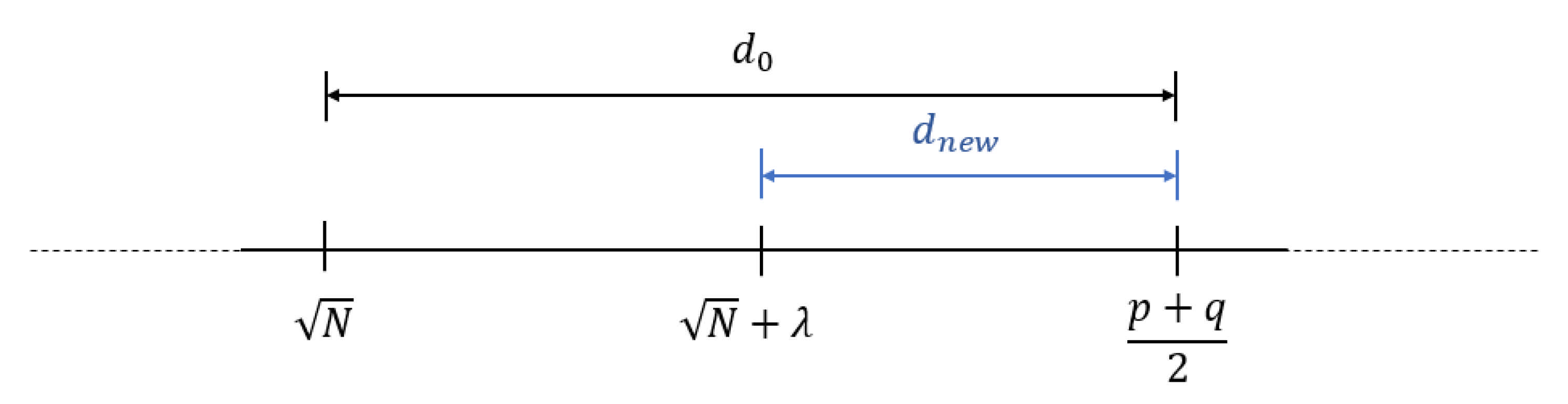
Question 1.

Is there any other potential initial values aside from $x=\sqrt{N}+\frac{h_t}{2}$ that can be selected to shorten the distance towards $\frac{p+q}{2}$?

Answer. 

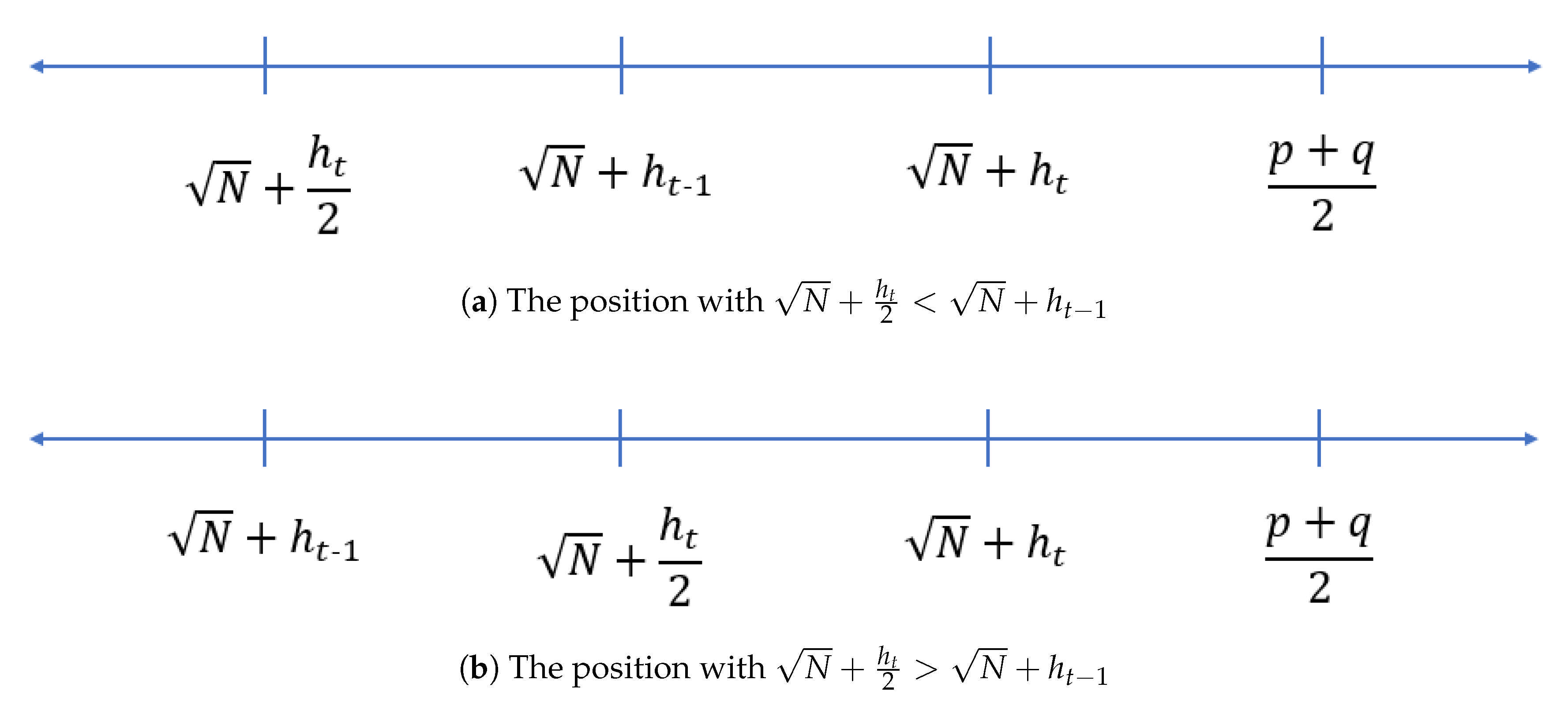
Interestingly, if we can find other candidates for initial values in which potentially reduces the distance $d_{new}$, then it can be useful to reduce the loop count to search for the value of $\frac{p+q}{2}$. Suppose the value of $\sqrt{N}+h_t$ is considered as the other candidate of potential values (i.e., the value of $\lambda$). Then, such value is supposed close to $\frac{p+q}{2}$. However, in general, it position is undecided whether $\sqrt{N}+h_t$ is larger (as shown by Figure 4) or is smaller than $\frac{p+q}{2}$ (i.e., similar to Lemma 1).

Figure 4. The position of $\sqrt{N}+h_t>\frac{p+q}{2}$.

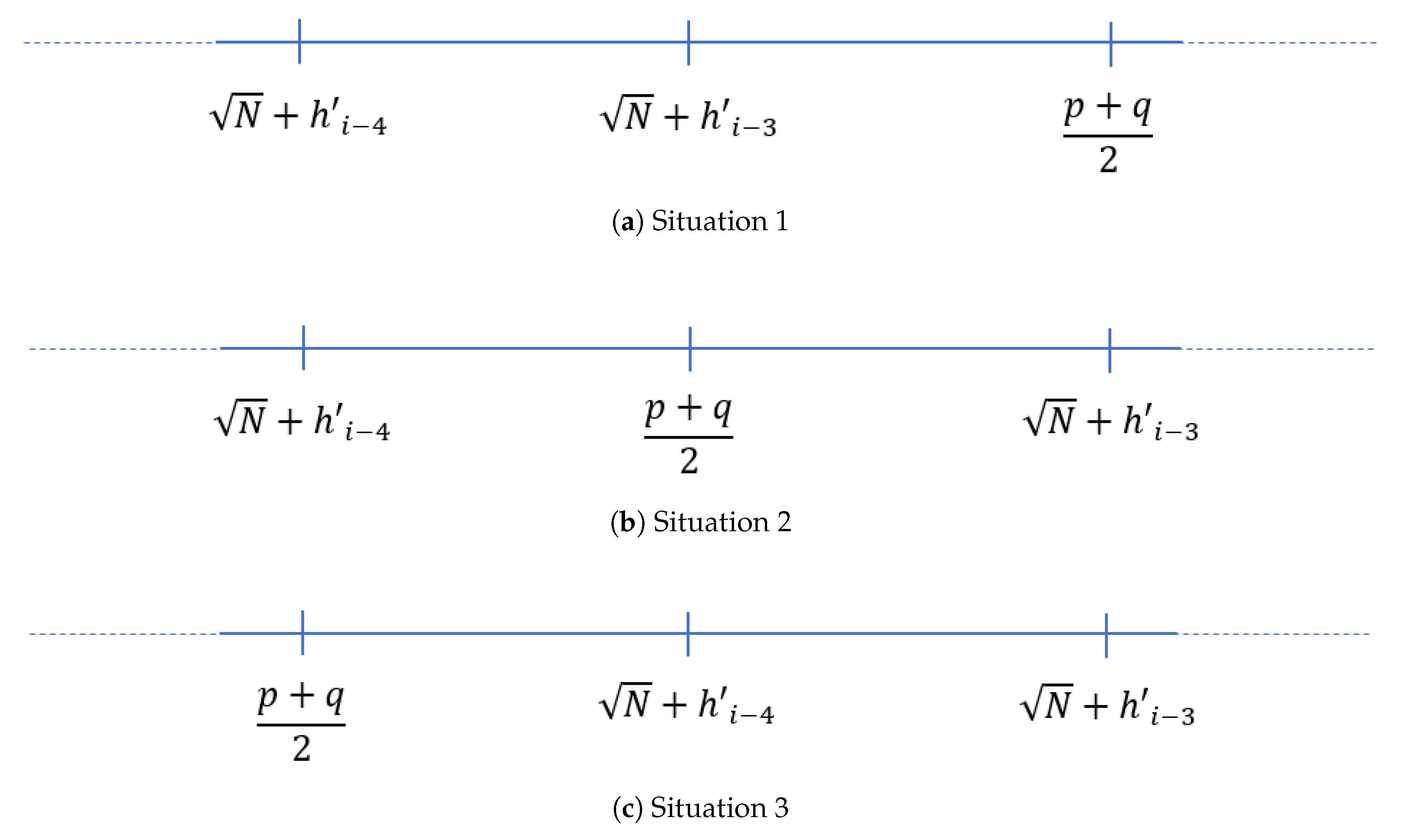
Next, suppose there exist $h_{t-1}$ such that $\frac{h_{t-1}}{k_{t-1}}$ is from the convergent list of $\frac{1}{\sqrt{N}}$ with $k_{t-1}<k_t\lesssim N$. By empirical evident, the value $\sqrt{N}+h_{t-1}<\frac{p+q}{2}$ can be considered as another candidate of additional extension for FFA1. Based on the empirical evident, it shows that the position of $\sqrt{N}+\frac{h_t}{2}$ and $\sqrt{N}+h_{t-1}$ are unpredictable as illustrated in Figure 5a,b.

Figure 5. The possible position between $\sqrt{N}+\frac{h_t}{2}$, $\sqrt{N}+h_{t-1}$, $\sqrt{N}+h_t$, and $\frac{p+q}{2}$.

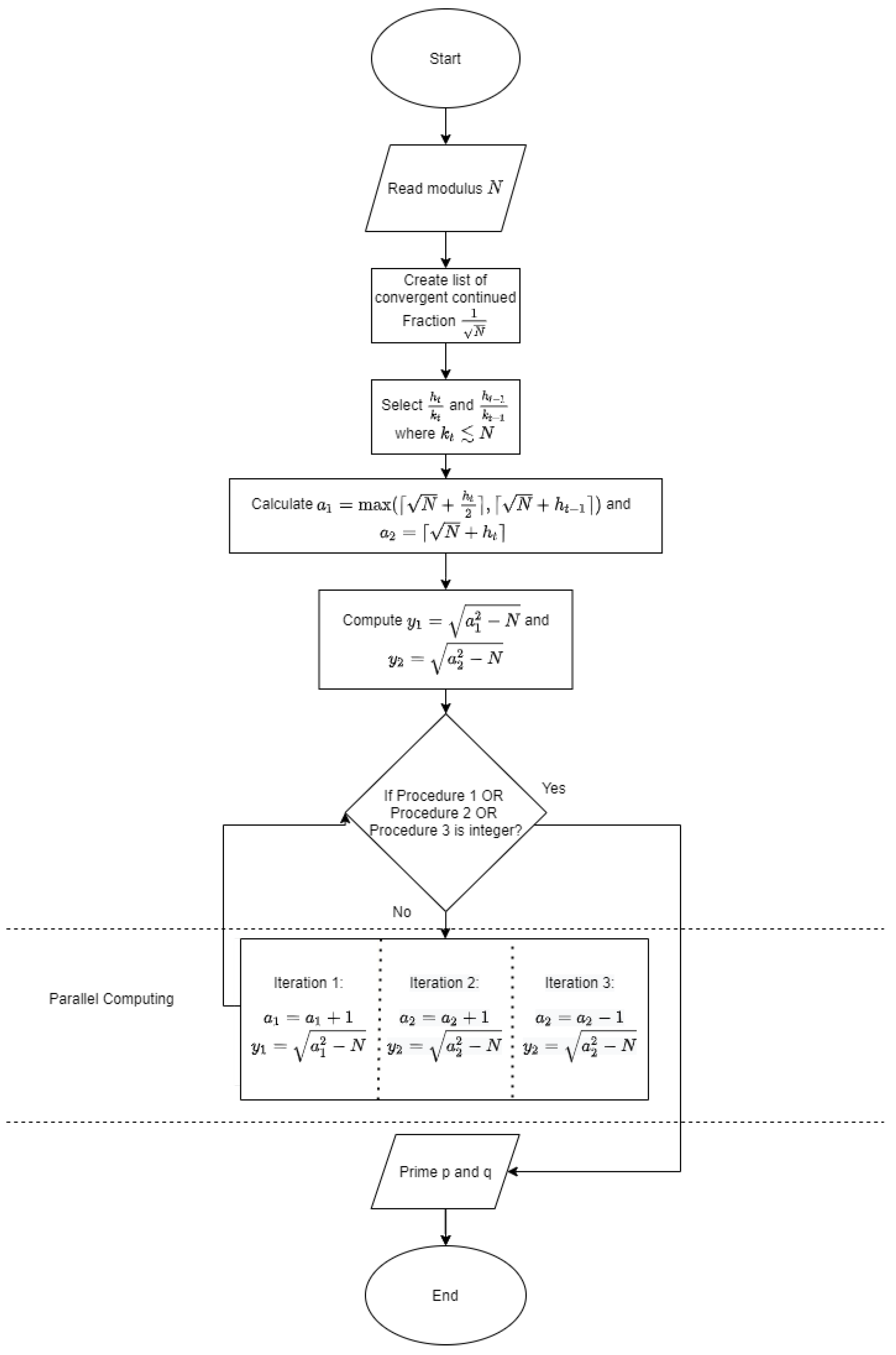
There are three candidates for the potential values for $\lambda$: $\frac{h_t}{2},h_{t-1},$ and $h_t$. In answering Question 1, the algorithm will start to compute the first value, $a_1=max\left(\lceil \sqrt{N}+h_{t-1}\rceil ,\lceil \sqrt{N}+\frac{h_t}{2}\rceil \right)$, while the second value is $a_2=\lceil \sqrt{N}+h_t\rceil$. Once $a_1$ and $a_2$ are established, then two values—$y_1=\sqrt{a_1^2-N}$ and $y_2=\sqrt{a_2^2-N}$—are computed.

After establishing the values of a’s and y’s, three procedures run simultaneously:

• Procedure 1: The iteration with potential initial value $a_1$ and $y_1$. The value $a_1$ is increased by 1 until $y_1$ is integer.
• Procedure 2: The iteration with potential initial value $a_2$ and $y_2$. The value $a_2$ is increased by 1 until $y_2$ is integer.
• Procedure 3: The iteration with potential initial value $a_2$ and $y_2$. The value $a_2$ is decreased by 1 until $y_2$ is integer.

Remark 3.

Note that the same value $a_2$ is applied in both Procedure 2 and Procedure 3. As the value $a_2,$ might be larger than $\frac{p+q}{2}$, the main role of Procedure 3 is to prevent the mFFA1-EPF algorithm to keep running forever. All of the procedure is done by parallel computing, which means that the algorithm will completely be stopped whenever one of the procedures outputs $y_1$ or $y_2$ as an integer. Eventually, p and q will be obtained.

Unbalanced prime is demonstrated in Algorithm 1 as follows and flowchart on Figure A1 in Appendix B.1.

Algorithm 1: mFFA1-EPF: Unbalanced Prime

Remark 4.

For the Type 2 case, Step 1 on Algorithm 1 is changed by selecting $\frac{h_i^{\prime }}{k_i^{\prime }}$ and $\frac{h_{i-1}^{\prime }}{k_{i-1}^{\prime }}$. Beside that, Step 3 will be modified with $a_1=max\left(\lceil \sqrt{N}+h_{i-1}^{\prime }\rceil ,\lceil \sqrt{N}+\frac{h_i^{\prime }}{2}\rceil \right)$ and $a_2=\lceil \sqrt{N}+h_i^{\prime }\rceil$.

Examples 1–4 are presented as illustrations of mFFA1-EPF for unbalanced primes. Example 1 demonstrates Type 1 of convergent-type selection, while Example 2 demonstrates Type 2 of convergent-type selection. Example 3 shows the importance of $a_2$ for this algorithm, and Example 4 shows the application of a previous example from Wu et al. [1].

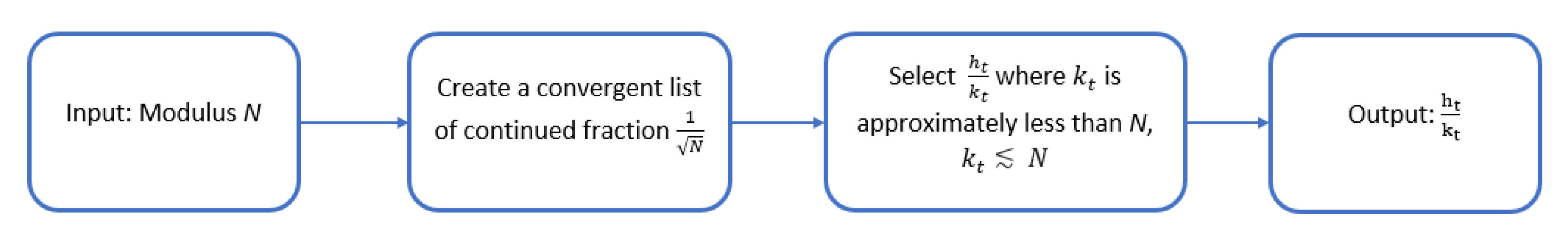
Example 1.

Let $N=\mathrm{707,896,463}$. By the continued fraction method, the following list of fraction $\frac{1}{\sqrt{N}}$ is created

$$\left[\dots ,\frac{34}{\mathrm{904,615}},\frac{139}{\mathrm{3,698,279}},\frac{\mathrm{33,811}}{\mathrm{899,586,412}},\dots \right]$$

We select $\frac{139}{\mathrm{3,698,279}}$ as a candidate of $\frac{h_t}{k_t}$ and $\frac{34}{\mathrm{904,615}}$ as a candidate of $\frac{h_{t-1}}{k_{t-1}}$ since $k_{t-1}<k_t\lesssim N$. Now, the potential initial values are computed as follows:

• $a_1=max\left(\lceil \sqrt{N}+h_{t-1}\rceil ,\lceil \sqrt{N}+\frac{h_t}{2}\rceil \right)=$ 26,676
• $a_2=\lceil \sqrt{N}+h_t\rceil =$ 26,746

With $a_1=\mathrm{26,676}$ and $a_2=\mathrm{26,746}$, Algorithm 1 is performed. The algorithm is stopped when Procedure 2 satisfy the searching on Algorithm 1 where $y_2$ become an integer $(y_2=\mathrm{66,126})$. Finally, $p=a_2+y_2=\mathrm{50,359}$ and $q=a_2-y_2=\mathrm{14,057}$ are computed.

Example 2.

Let $N=\mathrm{7,665,365,527,725,431}$. By continued fraction method, the following convergent list of $\frac{1}{\sqrt{N}}$ is created

$$\left[\dots ,\frac{1273}{\mathrm{111,453,789,228}},\frac{1554}{\mathrm{136,055,921,807}},\frac{2827}{\mathrm{247,509,711,035}}\right]$$

$\frac{2827}{\mathrm{247,509,711,035}}$ is selected as $\frac{h_i^{\prime }}{k_i^{\prime }}$ (the last convergent on the list) and $\frac{1554}{\mathrm{136,055,921,807}}$ as $\frac{h_{i-1}^{\prime }}{k_{i-1}^{\prime }}$ as $k_i^{\prime }<N$. The potential initial values are computed as follows:

• $a_1=max\left(\lceil \sqrt{N}+h_{i-1}^{\prime }\rceil ,\lceil \sqrt{N}+\frac{h_i^{\prime }}{2}\rceil \right)=\mathrm{87,553,628}$
• $a_2=\lceil \sqrt{N}+h_i^{\prime }\rceil =\mathrm{87,554,901}$

With $a_1=\mathrm{87,553,628}$ and $a_2=\mathrm{87,554,901}$, Algorithm 1 is performed. The algorithm is stopped when Procedure 2 satisfies the searching on Algorithm 1 where $y_2$ become an integer $(y_2=\mathrm{96,393,384})$. Last, $p=a_2+y_2=\mathrm{136,721,029}$ and $q=a_2-y_2=\mathrm{56,065,739}$ are computed.

Example 3.

Suppose $N=\mathrm{2,927,489,533}$. By continued fraction method, the following convergent list of $\frac{1}{\sqrt{N}}$ is created

$$\left[\dots ,\frac{5329}{\mathrm{288,332,366}},\frac{7097}{\mathrm{383,992,269}},\frac{12426}{\mathrm{672,324,635}}\right]$$

$\frac{\mathrm{12,426}}{\mathrm{672,324,635}}$ is selected as $\frac{h_i^{\prime }}{k_i^{\prime }}$ and $\frac{7097}{\mathrm{383,992,269}}$ as $\frac{h_{i-1}^{\prime }}{k_{i-1}^{\prime }}$ as $k_i^{\prime }<N$. Now, the potential initial values are computed as follows:

• $a_1=max\left(\lceil \sqrt{N}+h_{i-1}^{\prime }\rceil ,\lceil \sqrt{N}+\frac{h_i^{\prime }}{2}\rceil \right)=\mathrm{61,204}$
• $a_2=\lceil \sqrt{N}+h_i^{\prime }\rceil =\mathrm{66,533}$

With $a_1=\mathrm{29,682}$ and $a_2=\mathrm{36,369}$, Algorithm 1 is performed. The algorithm is stopped when Procedure 3 satisfies the searching on Algorithm 1 where $y_2$ become integer $(y_2=\mathrm{65,903})$. Last, $p=a_2+y_2=\mathrm{49,307}$ and $q=a_2-y_2=\mathrm{10,723}$ are computed.

Example 4.

Suppose $N=\mathrm{1,783,647,329}$ which adapted from the numerical example of Wu et al. [1]. By continued fraction method, the following convergent list of $\frac{1}{\sqrt{N}}$ is created

$$\left[\dots ,\frac{2758}{\mathrm{11,6479,301}},\frac{\mathrm{10,205}}{\mathrm{430,990,307}},\frac{\mathrm{12,963}}{\mathrm{547,469,608}},\dots \right]$$

$\frac{\mathrm{12,963}}{\mathrm{547,469,608}}$ is selected as a candidate of $\frac{h_t}{k_t}$ and $\frac{\mathrm{10,205}}{\mathrm{430,990,307}}$ as a candidate of $\frac{h_{t-1}}{k_{t-1}}$ since $k_{t-1}<k_t<N$. Two potential initial values are computed as follows:

• $a_1=max\left(\lceil \sqrt{N}+h_{t-1}\rceil ,\lceil \sqrt{N}+\frac{h_t}{2}\rceil \right)=\mathrm{52,439}$
• $a_2=\lceil \sqrt{N}+h_t\rceil =\mathrm{55,197}$

Algorithm 1 is performed and stop when Procedure 1 satisfies that $y_1$ is an integer $(y_1=\mathrm{31,664})$. Last, $p=a_1+y_1=\mathrm{84,449}$ and $q=a_1-y_1=\mathrm{21,121}$ are computed.

4.2. Discussion of Algorithm 1 (mFFA1-EPF: Unbalanced Primes)

This section presents a comparative analysis between the mFFA1-EPF and the previous technique, based on loop count and computational time. Note that all experimental results were using a computer running on 2.1 GHz on Intel® Core i3 with 4 GB of RAM.

According to Table 2, the loop count on Procedure 2 of Examples 1 and 2 is the shortest one. It shows that the mFFA1-EPF has the smallest loop count compared to the other methods. For Example 3, Procedure 3 has the shortest path (630), at the same time it indicates $\sqrt{N}+h_t$ is larger than $\frac{p+q}{2}$. Thus far, the results give a good visualization representing the factorization of modulus N by our method experimentally. Example 4 is the same example as given in Wu et al. [1]. Procedure 1 obtained the smallest loop count (346) compared to other methods. This N/A (Not Applicable) means that all the procedure in Algorithm 1 is stopped when one of the y’s from any procedures got the integer first.

Table 2. The comparison on loop count between FFA1, FFA2, and FFA2-EPF with our propose method toward Examples 1–4.

$\mathit{N}=\mathit{p}\mathit{q}$	FFA1	FFA2	FFA2-EPF	mFFA1-EPF
				Procedure 1	Procedure 2	Procedure 3
Example 1	128,439	386,939	342,627	N/A	120,265	N/A
Example 2	8,841,310	98,337,910	97,340,072	N/A	8,838,483	N/A
Example 3	11,796	98,844	33,091	N/A	N/A	630
Example 4 [1]	11455	42,215	10,551	346	N/A	N/A

The mFFA1-EPF is performed by parallel computing, which means Procedures 1–3 were run simultaneously. We recorded the computational time for the three different procedures. In Table 3, mFFA1-EPF is faster than FFA1 by 4 numerical examples. This seems to be a slight improvement for FFA1 as there is an involvement of additional extension. mFFA1-EPF is good in term of loop count, running without failure and computational time (compared to FFA1).

Table 3. The comparison on computational time in second (s) between FFA1, FFA2, and FFA2-EPF with mFFA1-EPF toward Examples 1–4.

$\mathit{N}=\mathit{p}\mathit{q}$	FFA1	FFA2	FFA2-EPF	mFFA1-EPF
				Procedure 1	Procedure 2	Procedure 3
Example 1	2.86	0.64	0.50	N/A	2.01	N/A
Example 2	338.12	215.89	199.27	N/A	301.98	N/A
Example 3	0.63	0.17	0.09	N/A	N/A	0.33
Example 4 [1]	0.55	0.12	0.10	0.23	N/A	N/A

To make mFFA1-EPF more convincing, there are numerical examples from Somsuk [6] provided in Table 4.

Table 4. The comparison loop count between FFA1, FFA2, FFA2-EPF, and FFA-Euler with our proposed method by Somsuk’s Example (Table 2 and Table 3 [6]).

Modulus N	FFA1	FFA2	FFA2-EPF	FFA-Euler	mFFA1-EPF
					Procedure 1	Procedure 2	Procedure 3
1,047,329,636,821,139,813 = 1,971,074,143 · 531,349,691	227,820,673	1,895,365,798	1,893,402,196	227,820,673	N/A	227,819,732	N/A
788,582,867,650,121,563 = 1,066,200,463· 739,619,701	14,888,197	356,357,156	307,600,540	14,888,197	N/A	14,236,836	N/A

This comparison highlights the improvement made by mFFA1-EPF compared to the method FFA-Euler, provided by Somsuk [6]. By two examples from in [6], the exhaustive search is improved with shortest loop counts, and the potential initial values are shorter than the FFA-Euler loop count. This shows that our method can be compatible with all unbalanced prime.

4.3. mFFA1-EPF: Balanced Prime

Previously, in the case of a modulus with unbalanced primes, three candidates are determined as the $\lambda$. Only two potential initial values that possibly shorten the $d_{n}ew$ were selected. In this section, we will explore the case of a modulus with balanced primes. The aim is to dictate the proper candidates from the convergent list (i.e., mFFA1-EPF) for the potential initial values via a similar approach.

Recall that $\frac{h_t}{k_t}$ with index t, where $k_t\lesssim N$, deemed as the indicator for selecting a good convergent to additional extension of initial values for FFA2-EPF [1]. When the EPF technique applied for the balanced prime case on FFA1, by empirical evidence, it shows that such indicator leads to the initial value ($\sqrt{N}+h_t$) relatively far away from the target value (exceeded by $\frac{p+q}{2}$). Therefore, we conjecture that the EPF method seems not to be an effective method to factor the modulus N with a balanced prime. Furthermore, the result in Somsuk [5] agreed that EPF is only suitable for unbalanced prime. It failed to address the convergent with index t as a suitable index to improve the initial value.

Therefore, in this section, we provide the strategies to address such drawback of factoring the modulus N with a balanced prime by imposing modification in the mFFA1-EPF algorithm. The strategies involve convergent selection and modification of potential initial values. Therefore, to enhance the effectiveness via mFFA1-EPF, the additional extension $h_t$ until $h_{t-5}$ is observe empirically to determine the smallest value of $d_{new}$. 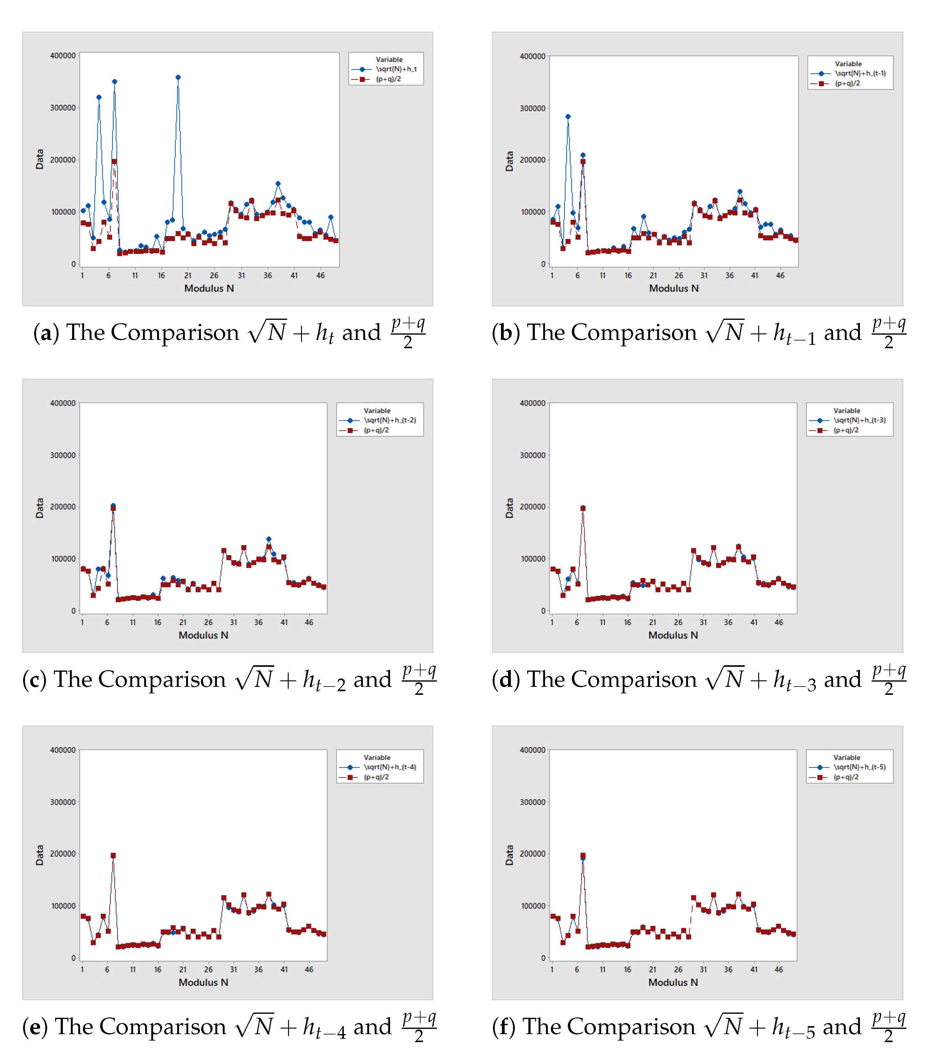The result of the observation is presented on Figure 6, and the discussion follows.

Figure 6. The comparison value of 50 data (distinct modulus N) between $h_t$, $h_{t-1}$, $h_{t-2}$, $h_{t-3}$, $h_{t-4}$ and $\frac{p+q}{2}$.

Suppose $\frac{h_t}{k_t}$ with index t where $k_t\lesssim N$ is chosen via EPF. Note that for the modulus N with balanced primes case, the value $\sqrt{N}+h_t\gg \frac{p+q}{2}$. Therefore, the additional extension from $h_t$ to $h_{t-5}$ is analysed. Interestingly, the additional extension $\sqrt{N}+h_{t-j}$ for $j=0,1,2,3,4,5$ can be a potential initial values as it moves closer to the value of $\frac{p+q}{2}$. Figure 6a–f shows comparison of potential initial values between the additional extension of $\sqrt{N}+h_{t-j}$ for $j=0,1,2,3,4,5$ and $\frac{p+q}{2}$, respectively. The potential initial values decrease, because the value of additional extension is become smaller from $h_t$ to $h_{t-5}$ (i.e., $h_t>h_{t-1}>h_{t-2}>h_{t-3}>h_{t-4}>h_{t-5}$).

Question 2.

What are the suitable initial values that need to be implemented on mFFA1-EPF with balanced primes?

Answer. 

Based on Figure 6, the line graph between the initial value (represented by the blue dots) starts closer to the target value $\frac{p+q}{2}$ (represented by the red dots) as the value of initial values changes. A hindrance to the development process for this approach is that we can not determine the smallest value of $d_{new}$ via additional extension $h_t$ to $h_{t-5}$. In other words, the “closeness” of the potential initial values with additional extension unable to be decided simply from the results of Figure 6. This is because the additional extension a random value from the generation of convergent list of $\frac{1}{\sqrt{N}}$. It requests further analysis. A statistical analysis of 50 distinct moduli N with balanced primes is conducted to determine the closeness of potential initial value through index t to $t-5$, as follows.

In this work, a measurement called Mahalanobis Distance (MD) is implemented. MD is the distance between two points in multivariate space. According to Çakmakçı et al. [15], MD measures the distance between a multidimensional point of probability distribution and distribution of distance. The smaller the value of MD, the closer the mean of candidate of potential initial values to the mean of the target value.

In the one-dimensional case on the mFFA1-EPF for balanced prime, MD is used to calculate the normalized distance between the mean of each $h_t$ to $h_{t-5}$ and the mean of the target value $\frac{p+q}{2}$. The measurement formula is

$$\begin{array}{c}\hfill \mathrm{MD}=\frac{|{\mu }_{IV}-{\mu }_{AV}|}{{\sigma }_{IV+AV}}\end{array}$$

(5)

where ${\mu }_{IV}$ is a mean of each data potential initial value of $\sqrt{N}+h_t$ to $\sqrt{N}+h_{t-5}$ while ${\mu }_{AV}$ is mean of actual value $\frac{p+q}{2}$. The value ${\sigma }_{IV+AV}$ is calculated from combination data from potential initial value and the actual value $\frac{p+q}{2}$. The following formula is represented for MD between $\sqrt{N}+h_t$ and $\frac{p+q}{2}$,

$${\mathrm{MD}}_{\left(\sqrt{N}+h_t\right)}=\frac{\left|{\mu }_{IV\left(\sqrt{N}+h_t\right)}-{\mu }_{AV}\right|}{{\sigma }_{IV+AV}}$$

We calculate MD for $\sqrt{N}+h_t$ to $\sqrt{N}+h_{t-5}$ by same data of 50 moduli N and represent the MD value on Table 5.

Table 5. The comparison on the closeness of value between the candidate of potential initial value with $\frac{p+q}{2}$ by MD.

Mahalanobis Distance (MD)	Value
${\mathrm{MD}}_{\left(\sqrt{N}+h_t\right)}$	0.4965
${\mathrm{MD}}_{\left(\sqrt{N}+h_{t-1}\right)}$	0.2932
${\mathrm{MD}}_{\left(\sqrt{N}+h_{t-2}\right)}$	0.0756
${\mathrm{MD}}_{\left(\sqrt{N}+h_{t-3}\right)}$	0.0114
${\mathrm{MD}}_{\left(\sqrt{N}+h_{t-4}\right)}$	0.0116
${\mathrm{MD}}_{\left(\sqrt{N}+h_{t-5}\right)}$	0.0257

Table 5 shows the comparison of the MD index of “closer distance” between several potential initial values from $h_t$ to $h_{t-5}$ and $\frac{p+q}{2}$. Table 5 reported that the MD index value of $\sqrt{N}+h_{t-3}$ and $\sqrt{N}+h_{t-4}$ are the smallest MD values among other potential initial values, that is, 0.0114 and 0.0116, respectively. It means that $\sqrt{N}+h_{t-3}$ and $\sqrt{N}+h_{t-4}$ are the most suitable candidates for potential initial values, because they have the smallest $d_{new}$ on average with respect to MD measurement.

Observation 3.

The candidates $\sqrt{N}+h_{t-3}$ and $\sqrt{N}+h_{t-4}$ have the smallest value of MD. Therefore, it is highly suggested to select convergents with index $t-3$ and $t-4$ to improve the initial values.

Based on Observation 3, two potential initial values are set as follows:

• $b_1=\sqrt{N}+h_{t-3}$
• $b_2=\sqrt{N}+h_{t-4}$

Remark that the FFA1 algorithm requires an initial value less than the target value and will keep increasing by one (i.e., +1) until it reaches $\frac{p+q}{2}$. Therefore, in mFFA1-EPF, we use the variation technique, which means the value of $b_1$ and $b_2$ need to be increased and decreased by 1 simultaneously. Next, the following values are established:

• $y_1=\sqrt{b_1^2-N}$
• $y_2=\sqrt{b_2^2-N}$

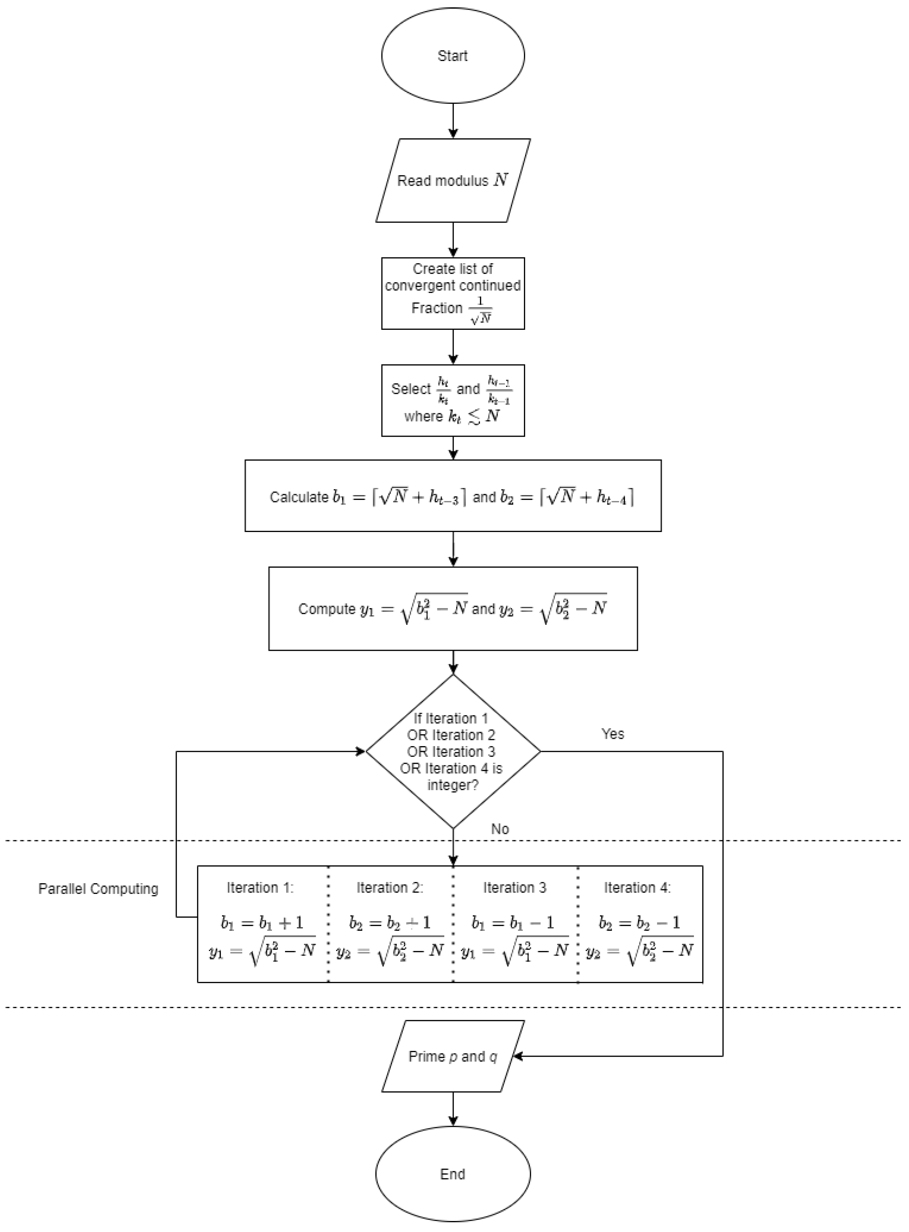
Four procedures are introduced using the above values, with the variation technique as follows:

• Procedure 1: The iteration with potential initial values $b_1$ and $y_1$. The value of $b_1$ is increased by 1 until it is the same as the $y_1$ becomes an integer.
• Procedure 2: The iteration with potential initial values $b_2$ and $y_2$. The value of $b_2$ is increased by 1 until it is the same as $y_2$ becomes an integer.
• Procedure 3: The iteration with potential initial values $b_1$ and $y_1$. The value of $b_1$ is decreased by 1 until it is the same as the $y_1$ becomes an integer.
• Procedure 4: The iteration with potential initial values $b_2$ and $y_2$. The value of $b_2$ is decreased by 1 until it is the same as the $y_2$ becomes an integer.

Note that these four procedures were run simultaneously by parallel computing which will stop when one of the y’s become the first integer. Algorithm 2 shows how the workflow runs.

Algorithm 2: mFFA1-EPF: Balanced Prime

4.4. Discussion on Algorithm 2 (mFFA1-EPF: Balanced Primes)

Algorithm 2 is also illustrated as a flowchart in Figure A2 in Appendix B.2. The experimental result is represented using the mFFA1-EPF via balanced prime on Example 5 while applying mFFA1-EPF is represented on Somsuk’s numerical example [6] in Example 6.

Example 5.

(Procedure 1 satisfies on Example 5). Let $N=\mathrm{616,696,115,591}$. By continued fraction method, the following convergent list $\frac{1}{\sqrt{N}}$ is created

$$\left[\dots ,\frac{61}{\mathrm{47,903,301}},\frac{123}{\mathrm{96,591,902}},\frac{184}{\mathrm{144,495,203}},\frac{491}{\mathrm{385,582,308}},\dots \right]$$

$\frac{491}{\mathrm{385,582,308}}$ is selected as a candidate of $\frac{h_{t-3}}{k_{t-3}}$ and $\frac{184}{\mathrm{144,495,203}}$ as a candidate of $\frac{h_{t-4}}{k_{t-4}}$ since $k_{t-4}<k_{t-3}<k_t\lesssim N$. Now, there are two candidates of potential initial value and 2 y’s are computed as follows:

• $b_1=\lceil \sqrt{N}+h_{t-3}\rceil =\mathrm{785,792}$
• $b_2=\lceil \sqrt{N}+h_{t-4}\rceil =\mathrm{785,485}$

Algorithm 2 is performed because $y_1$ and $y_2$ not integers. The values $b_1$ and $b_2$ in Procedure 1 and 2 are increased by 1 while initial values in Procedure 3 and 4 are decreased by 1. The algorithm stop where $y_1$ from Procedure 1 is integer $(y_1=\mathrm{801,204})$. Finally, compute $p=b_1+y_1=\mathrm{960,049}$ and $q=b_1-y_1=\mathrm{642,359}$.

Example 6.

[6] (Procedure 1 satisfies on Example 6) Say $N=\mathrm{340,213}$. By continued fraction method, a list of fraction $\frac{1}{\sqrt{N}}$ is created

$$\left[\dots ,\frac{1}{583},\frac{3}{1750},\frac{4}{2333},\frac{7}{4083},\dots \right]$$

$\frac{3}{1750}$ is selected as a candidate of $\frac{h_{t-3}}{k_{t-3}}$ and $\frac{1}{583}$ as a candidate of $\frac{h_{t-4}}{k_{t-4}}$ since $k_{t-4}<k_{t-3}<k_t<N$. Now, there are two candidates of potential initial value and 2 y’s are computed as follows:

• $b_1=\lceil \sqrt{N}+h_{t-3}\rceil =587$
• $b_2=\lceil \sqrt{N}+h_{t-4}\rceil =585$

Algorithm 2 is performed because $y_1$ and $y_2$ not integer. The values $b_1$ and $b_2$ in Procedure 1 and 2 are increased by 1 while initial values in Procedure 3 and 4 are decreased by 1. The algorithm stop where $y_1$ from Procedure 1 is integer $(y_1=587)$. We compute $p=b_1+y_1=653$ and $q=b_1-y_1=521$.

Table 6 shows the comparison on count loop and computational time in seconds (s), between several FFAs with our proposed method toward Example 5. The loop count on Procedure 1 (15412) is the least number of loop count compared to previous methods. Besides, FFA2-EPF can not undergo the process and the loop count is not available since the initial value exceeded the value of $p+q$ and $p-q$. When it goes on computational time, the algorithm is not shown the fastest one but it still improves from FFA1.

Table 6. The comparison on loop count and computational time in second (s) between several FFAs with our propose method toward Example 5.

Example 5	FFA1	FFA2	FFA2-EPF	mFFA1-EPF
				Procedure 1	Procedure 2	Procedure 3	Procedure 4
Loop count	15,903	174,748	N/A	15,412	N/A	N/A	N/A
Computational time, s	0.71	0.2	N/A	0.48	N/A	N/A	N/A

For Table 7, mFFA1-EPF is applied toward [6] to compare the loop count and computational time. It shows the shortest loop count even the initial value is exactly the value of $\frac{p+q}{2}$ ($\frac{p+q}{2}=\sqrt{N}+h_{t-3}=587$). Using Algorithm 2, the loop count reduced significantly, which result in the exhaustive search to run without fail.

Table 7. The comparison on loop count and computational time in second (s) between several FFAs with our propose method toward Example 6 [6].

Example 6	FFA1	FFA2	FFA2-EPF	FFA-Euler	mFFA1-EPF
					Procedure 1	Procedure 2	Procedure 3	Procedure 4
Loop count	3	6	N/A	3	0	N/A	N/A	N/A
Computational time, s	$2.12\times {10}^{-2}$	$1.45\times {10}^{-2}$	N/A	$7.89\times {10}^{-3}$	$4.92\times {10}^{-2}$	N/A	N/A	N/A

Remark 5.

Consider Type 2 of the continued fraction convergent selection of the modulus N with balanced primes. For Type 2, we use Algorithm 2 with a changes in Step 2 where $h_{i-3}^{\prime }$ and $h_{i-4}^{\prime }$ and $k_i^{\prime }<N$.

Now, we replicate a numerical example from the Algorithm 2 with respect to Remark 5 on Example 7.

Example 7.

(Procedure 4 satisfies on Example 7). Suppose $N=\mathrm{9,355,908,869}$. By continued fraction method, a convergent list of $\frac{1}{\sqrt{N}}$ is created

$$\left[\dots ,\frac{1611}{\mathrm{155,825,501}},\frac{2009}{\mathrm{194,322,428}},\frac{3620}{\mathrm{350,147,929}},\frac{9249}{\mathrm{894,618,286}},\frac{\mathrm{22,118}}{\mathrm{2,139,384,501}}\right]$$

As $\frac{h_i^{\prime }}{k_i^{\prime }}$ is the last convergent on the list, $\frac{2009}{\mathrm{194,322,428}}$ is selected as a candidate of $\frac{h_{i-3}^{\prime }}{k_{i-3}^{\prime }}$ and $\frac{1611}{\mathrm{155,825,501}}$ as a candidate of $\frac{h_{i-4}^{\prime }}{k_{i-4}^{\prime }}$ as $k_{i-4}^{\prime }<k_{i-3}^{\prime }<k_i^{\prime }<N$. We compute two candidates of initial value of x, $y_1$ and $y_2$ as follows:

• $b_1=\lceil \sqrt{N}+h_{i-3}^{\prime }\rceil =\mathrm{98,735}$
• $b_2=\lceil \sqrt{N}+h_{i-4}^{\prime }\rceil =\mathrm{98,337}$

Since $y_1$ and $y_2$ are not integer, the values $b_1$ and $b_2$ in Procedures 1 and 2 are increased by 1 while initial values in Procedures 3 and 4 are decreased by 1. The algorithm stop where $y_2$ in Procedure 4 is integer $(y_2=\mathrm{97,245})$. We compute $p=b_2+y_2=\mathrm{107,279}$ and $q=b_2-y_2=\mathrm{87,211}$.

Table 8 shows the comparison on loop count and computational time in second between several FFAs with our propose method toward Example 7. Procedure 4 shows the smallest loop count with 1092 compared to FFA1 (1590) and FFA2 (10,553). The loop count of FFA2-EPF is unavailable as the initial values are exceeded the value of $p+q$ and $p-q$. On computational time, our algorithm is slightly better than FFA1. Procedure 4 plays it crucial part to achieve the value $\frac{p+q}{2}$, and, at the same time, Procedure 4 obtains the indicators of whether the value is larger or smaller than $\frac{p+q}{2}$. Therefore, Algorithm 2 with Remark 5 helps to search for the value of $\frac{p+q}{2}$ without failure.

Table 8. The comparison on loop count and computational time in second (s), between several FFAs with our propose method toward Example 7.

Example 7	FFA1	FFA2	FFA2-EPF	mFFA1-EPF
				Procedure 1	Procedure 2	Procedure 3	Procedure 4
Loop count	1590	10553	N/A	N/A	N/A	N/A	1092
Computational time, s	8.90 × ${10}^{-2}$	1.90 × ${10}^{-2}$	N/A	N/A	N/A	N/A	4.07× ${10}^{-2}$

Recall that there is $d_{new}=\frac{p+q}{2}-(\sqrt{N}+\lambda )$. For mFFA1-EPF, the $\lambda$ varies according to type of modulus N; $\lambda =h_t$ and $\lambda =h_{t-1}$ for a modulus with unbalanced primes while $\lambda =h_{t-3}$ and $\lambda =h_{t-4}$ for a modulus with balanced primes. Multiple $\lambda$ can lead to the shortest path toward $\frac{p+q}{2}$. For comparison on mFFA1-EPF with FFA1, both methods use the same process of calculating the square roots to reach the target value $\frac{p+q}{2}$. However, mFFA1-EPF uses the additional extension on its potential initial values $d_{new}<d_0$ where $d_0$ is the loop count of FFA1. Based on the empirical results in this work, the loop count and computational time of mFFA1-EPF are improved compared to FFA1. Consequently, it reduces the cost of running the exhaustive search.

The uniqueness of FFA2 is that it uses multiplication operation as the main process, it has less cost in computational time compared to the mFFA1-EPF which uses square root operation. Alas, FFA2 requires a greater number of iterations to achieve $p+q$ and $p-q$. In this regard, the mFFA1-EPF uses less cost in terms of computational memory and less space to run the iteration compared to FFA2.

The objective of establishing additional extension on FFA2-EPF is the same as mFFA1-EPF, to shorten the path toward $p+q$ and $p-q$. mFFA1-EPF has a shorter loop count than FFA2-EPF because the main operation comes from FFA2, which uses a huge number of iteration to achieve its target values: $p+q$ and $p-q$. Thus, mFFA1-EPF requires less cost in terms of space compared to FFA2-EPF.

5. Conclusions and Future Works

In this study, we discovered two types of convergent list selections. The first is Type 1: $\frac{h_t}{k_t}$ is selected from the convergent list of $\frac{1}{\sqrt{N}}$ where $k_t\lesssim N$. For Type 1, Wu et al. [1] mentioned that $\frac{h_t}{k_t}$ can be an indicator of convergent with index t to select a good candidate for initial value. Next, Type 2: $\frac{h_i^{\prime }}{k_i^{\prime }}$ where $k_i^{\prime }$ is the last convergent on the list (as illustrated by Figure 4) where $h_i^{\prime }$ will be selected for additional extension for potential initial value. This paper proposed two improved factoring algorithms called mFFA1-EPF for unbalanced primes and mFFA1-EPF for balanced primes. The general idea for designing the algorithms is due to a modification made to EPF and then implemented to (improved) FFA1. The resulting study shows a significant improvement that reduces the loop count of FFA1 via (improved) EPF compared to previous methods (FFA1, FFA2, FFA2-EPF, and FFA-Euler).

An interesting limitation to our work is that the computational time of mFFA1-EPF is still far beyond efficient to factor a modulus with 1024-bit size of balanced primes, with the current technology. We foresee that the mFFA1-EPF might be useful once a large quantum computer with stable qubits is available. The mFFA1-EPF is a type of searching algorithm, thus it might take advantage of making fine adjustments or manipulating the mathematical nature within Grover’s searching quantum algorithm [16]. The mFFA1-EPF can be used in machine architecture with low power such as the Internet of Things-based devices, which requires to factor small composites integer [1,9]. Furthermore, we expect mFFA1-EPF to be an assistive tool to increase the effort on the machine learning and artificial intelligence approaches, such as in [17], have been introduced in the literature to deal with similar problems as ours.

Appendix B.1. mFFA1-EPF on Unbalanced Prime

Figure A1. The flowchart of mFFA1-EPF on unbalanced prime.

Figure A1. The flowchart of mFFA1-EPF on unbalanced prime.

Appendix B.2. mFFA1-EPF on Balanced Prime

Figure A2. The flowchart of mFFA1-EPF on balanced prime.

Figure A2. The flowchart of mFFA1-EPF on balanced prime.