Lyapunov Functions and Lipschitz Stability for Riemann–Liouville Non-Instantaneous Impulsive Fractional Differential Equations

Abstract

In this paper a system of nonlinear Riemann–Liouville fractional differential equations with non-instantaneous impulses is studied. We consider a Riemann–Liouville fractional derivative with a changeable lower limit at each stop point of the action of the impulses. In this case the solution has a singularity at the initial time and any stop time point of the impulses. This leads to an appropriate definition of both the initial condition and the non-instantaneous impulsive conditions. A generalization of the classical Lipschitz stability is defined and studied for the given system. Two types of derivatives of the applied Lyapunov functions among the Riemann–Liouville fractional differential equations with non-instantaneous impulses are applied. Several sufficient conditions for the defined stability are obtained. Some comparison results are obtained. Several examples illustrate the theoretical results.

1. Introduction

Fractional differential equations have attracted considerable attention due to their many applications in science and engineering (see the monographs [1,2,3,4] and the references therein). The main advantage of fractional derivatives is that they can describe the properties of heredity and memory of many materials. There are various types of fractional derivatives known in the literature. One of the most important properties of the solutions is stability. There are various types of stability that describe different properties of the solutions. One of them is Lipschitz stability, defined and studied for ordinary differential equations in [5]. Later, this type of stability was studied for various types of differential equations and problems, such as nonlinear differential systems [6,7,8], impulsive differential equations with delays [9], fractional differential systems [10], Caputo fractional differential equations with non-instantaneous impulses [11], a piecewise linear Schrödinger potential [12], a hyperbolic inverse problem [13], the electrical impedance tomography problem [14], the radiative transport equation [15] and neural networks with non-instantaneous impulses [16].

In this paper we define and study Lipschitz stability for Riemann–Liouville (RL) fractional differential equations with non-instantaneous impulses. We will initially introduce the statement of the problem.

Let two sequences of points ${\left\{t_i\right\}}_{i=0}^{\infty }$, $t_0=0$, and ${\left\{s_i\right\}}_{i=0}^{\infty }$ be given such that $t_k<s_k<t_{k+1}<s_{k+1},k=0,1,2,\dots ,$ and ${lim}_{i\to \infty }{t}_i=\infty$.

There are mainly two types of impulses involved in differential equations: instantaneous impulses (known as impulses), where time of action is negligibly small comparatively with the whole duration of the process and non-instantaneous impulses that start their actions abruptly and continue to act on a finite interval.

In this paper we will consider the non-instantaneous impulses starting at points $s_i,i=0,1,2,\dots$ and acting on intervals $(s_i,t_{i+1}),i=0,1,2,\dots$. The intervals $(s_i,t_{i+1}),i=0,1,2,\dots$ will be called impulsive intervals. In addition, we will consider the RL fractional derivatives with changeable lower limits at each stop time point $t_i,i=0,1,2,\dots$ of the impulsive action.

The presence of the RL fractional derivative leads to two particular types of initial conditions that are equivalent (see the classical book [2]):

-

integral form of the initial condition

$${}_0{I}_t^{1-q}{x\left(t\right)|}_{t=0}=x_0.$$

-

weighted form of the initial condition

$$\underset{t\to 0+}{lim}\left(t^{1-q}x\left(t\right)\right)=\frac{x_0}{\Gamma \left(q\right)}.$$

Following the ideas of the impulses in ordinary differential equations, i.e., after the impulse the differential equation is the same with a new initial condition, the integral form and weighted form of the impulsive conditions can be defined.

In this paper we will use the integral form of both the initial condition and the impulsive conditions.

Keeping in mind the above description, in this paper we will study the initial value problem (IVP) for the following system of nonlinear RL fractional differential equations with non-instantaneous impulses (NIRLFDE) of fractional order $q\in (0,1)$:

$$\begin{array}{cc}& {}_{t_i}^{RL}{D}_t^{q}x\left(t\right)=f(t,x\left(t\right))\mathrm{for}t\in (t_i,s_i],i=0,1,2,\dots ,\hfill \\ & \underset{t\to t_i+}{lim}\left[{(t-t_i)}^{1-q}x\left(t\right)\right]=\frac{{\Psi }_{i-1}(t_i,x(s_{i-1}-0))}{\Gamma \left(q\right)},\mathrm{for}i=1,2,\dots ,\hfill \\ & x\left(t\right)={\Psi }_i(t,x(s_i-0))\mathrm{for}t\in (s_i,t_{i+1}],i=0,1,2,\dots .\hfill \\ & \underset{t\to 0+}{lim}\left[t^{1-q}x\left(t\right)\right]=\frac{x_0}{\Gamma \left(q\right)},\hfill \end{array}$$

(1)

where $x\in {\mathbb{R}}^n$ and ${}_0^{RL}{D}_t^{q}x\left(t\right)$ is the Riemann–Liouville fractional derivative.

Remark 1.

Both given sequences ${\left\{t_i\right\}}_{i=0}^{\infty }$ and ${\left\{s_i\right\}}_{i=0}^{\infty }$ divide the positive real line into two types of intervals: the intervals $(t_k,s_k],k=0,1,2,\dots ,$ on which the differential equation is given, and the impulsive intervals $(s_k,t_{k+1}],k=0,1,2,\dots ,$.

Remark 2.

The equality ${lim}_{t\to t_i+}\left[{(t-t_i)}^{1-q}x\left(t\right)\right]=\frac{{\Psi }_{i-1}(t_i,x(s_{i-1}-0))}{\Gamma \left(q\right)}$ could be replaced by ${lim}_{t\to t_i+}\left[{(t-t_i)}^{1-q}x\left(t\right)\right]=\frac{x(t_i-0)}{\Gamma \left(q\right)}.$

Remark 3.

For $q\to 1$ the impulsive condition ${lim}_{t\to t_i+}\left[{(t-t_i)}^{1-q}x\left(t\right)\right]=\frac{{\Psi }_{i-1}(t_i,x(s_{i-1}-0))}{\Gamma \left(q\right)}$ in Equation (1) is reduced to $x(t_i+)={\Psi }_{i-1}(t_i,x(s_{i-1}-0))$, which is an impulsive condition for ordinary differential equations with impulses (see the book [17]).

Note that the solutions of the IVP for the NIRLFDE of Equation (1) have singularities at each point $t_i,i=0,1,2,\dots$. This requires stability properties to be studied at intervals excluding these points. In this paper we will define a new type of Lipschitz stability for NIRLFDE of the type in Equation (1), which is an appropriate generalization of the classical Lipschitz stability introduced in [5]. It is called generalized Lipschitz stability in time. This type of stability is connected with the singularity of the solution at both the initial time point and the stop time points of impulses. In connection with this we consider an interval excluding these time points. We use Lyapunov functions and two types of derivatives of these Lyapunov functions among the studied RL fractional equation with non-instantaneous impulses. Several sufficient conditions for Lipschitz stability in time are obtained. Some examples illustrating the theoretical results and comparing the application of both fractional derivatives of Lyapunov functions are given.

We will use the following sets:

$$\begin{array}{cc}\hfill C_{1-q}([a,b],{\mathbb{R}}^n)=& \left\{u:(a,b]\to {\mathbb{R}}^n:u\in C((a,b),{\mathbb{R}}^n),\underset{t\to a+}{lim}{(t-a)}^{1-q}u\left(t\right)<\infty \right\},\hfill \\ \hfill P{C}_{1-q}([0,\infty ),{\mathbb{R}}^n)=& \{u:(0,\infty )\to {\mathbb{R}}^n:u\in C\left(\mathcal{J},{\mathbb{R}}^n\right),\hfill \\ & u\left(t_k\right)=u(t_k-0)=\underset{\epsilon \to 0+}{lim}u(t_k-\epsilon )<\infty ,k=1,2,\dots ,\hfill \\ & u\left(s_k\right)=u(s_k-0)=\underset{\epsilon \to 0+}{lim}u(s_k-\epsilon )<\infty ,k=0,1,2,\dots ,\hfill \\ & \underset{t\to t_k+}{lim}{(t-t_k)}^{1-q}u\left(t\right)<\infty ,k=0,1,\dots \},\hfill \end{array}$$

where $\mathcal{J}=\left({\cup }_{k=0}^{\infty }(t_k,s_k]\right)\bigcup \left({\cup }_{k=0}^{\infty }(s_k,t_{k+1}]\right)$, $a,b\in {\mathbb{R}}_{+}:a>b$.

Remark 4.

If $u\in P{C}_{1-q}([0,\infty ),{\mathbb{R}}^n)$ then for any $k=0,1,2,\dots$ we get $u\in C_{1-q}([t_k,s_k],{\mathbb{R}}^n)$.

The main contributions of the paper can be summarized as follows:

-

for a nonlinear system with RL fractional derivatives of order $q\in (0,1)$ and non-instantaneous impulses we define in an appropriate way both the initial condition and the non-instantaneous impulsive conditions;

-

generalized Lipschitz stability in time of the zero solution of a system of nonlinear RL fractional differential equations with non-instantaneous impulses is defined;

-

two types of derivatives of Lyapunov functions among the RL fractional differential equations with non-instantaneous impulses are applied;

-

comparison results with Lyapunov functions, scalar RL fractional equations with non-instantaneous impulses and both types of derivatives of Lyapunov functions are proved;

-

sufficient conditions for generalized Lipschitz stability in time are obtained by the application of both types of derivatives of Lyapunov functions.

2. Preliminaries

In this section we will give the definitions of fractional derivatives used in the paper (see, for example, [1,2,3]). These definitions are given for scalar functions but they also are easily generalized to the vector case by taking fractional derivatives component-wisely. Throughout the paper we will assume $q\in (0,1)$.

-

Riemann–Liouville (RL) fractional integral:

$${}_a{I}_t^{1-q}m\left(t\right)=\frac{1}{\Gamma \left(1-q\right)}\underset{a}{\overset{t}{\int }}\frac{m\left(s\right)}{{(t-s)}^q}ds,t>a,$$

where $\Gamma (.)$ denotes the Gamma function;

-

Riemann–Liouville fractional derivative:

$${}_a^{RL}{D}_t^{q}m\left(t\right)=\frac{1}{\Gamma \left(1-q\right)}\frac{d}{dt}\underset{a}{\overset{t}{\int }}{\left(t-s\right)}^{-q}m\left(s\right)ds,t>a;$$

-

The Grünwald–Letnikov fractional derivative is given by

$${}_a^{GL}{D}_t^{q}m\left(t\right)=\underset{h\to 0}{lim}\frac{1}{h^q}\sum _{r=0}^{\left[\frac{t-a}{h}\right]}{\left(-1\right)}^r{}_q{C}_{r}m\left(t-rh\right),t>a,$$

and the Grünwald–Letnikov fractional Dini derivative by

$${}_a^{GL}{D}_{+}^{q}m\left(t\right)=\underset{h\to 0+}{lim\; sup}\frac{1}{h^q}\sum _{r=0}^{\left[\frac{t-a}{h}\right]}{(-1)}^r{}_q{C}_{r}m(t-rh),t>a,$$

(2)

where ${}_q{C}_r=\frac{q(q-1)\dots (q-r+1)}{r!}$ and $\left[\frac{t-a}{h}\right]$ denotes the integer part of the fraction $\frac{t-a}{h}>0$.

Remark 5.

If $m\in C\left(\right[a,a+T],\mathbb{R})$, then ${}_a^{RL}{D}_t^{q}m\left(t\right)={}_a^{GL}{D}_t^{q}m\left(t\right)={}_a^{GL}{D}_{+}^{q}m\left(t\right)$ hold (see Theorem 2.25 [2]).

Proposition 1

(Lemma 2.3 [18]). Let $m\in C_{1-q}([a,a+T),\mathbb{R})$. Suppose that for an arbitrary $t_1\in (a,a+T)$, we have $m\left(t_1\right)=0$ and $m\left(t\right)<0$ for $a\le t<t_1$. Then it follows that ${}_a^{RL}{D}_t^q{m\left(t\right)|}_{t=t_1}\ge 0$.

Remark 6.

From Remark 5 it follows that in Proposition 1 the fractional derivative could be replaced by ${}_a^{GL}{D}_t^q{m\left(t\right)|}_{t=t_1}$.

The practical definition of the initial condition as well as the impulsive conditions of fractional differential equations with RL derivatives is based on the following result:

Proposition 2

([2]). Let $q\in (0,1)$ and $a,T>0$, $m:[a,a+T]\to \mathbb{R}$ be a Lebesgue measurable function.

(a) 

If there exists a.e. a limit ${lim}_{t\to a+}\left[{(t-a)}^{1-q}m\left(t\right)\right]=c\in \mathbb{R}$, then there also exists a limit

$${}_a{I}_t^{1-q}{m\left(t\right)|}_{t=a}:=\underset{t\to a+}{lim}\frac{1}{\Gamma \left(1-q\right)}\underset{a}{\overset{t}{\int }}\frac{m\left(s\right)}{{(t-s)}^q}ds=c\Gamma \left(q\right)=\Gamma \left(q\right)\underset{t\to a+}{lim}\left[{(t-a)}^{1-q}m\left(t\right)\right].$$

(b) 

If there exists a.e. ${}_a{I}_t^{1-q}{m\left(t\right)|}_{t=a}=c\in \mathbb{R},$ and if there exists ${lim}_{t\to a+}\left[{(t-a)}^{1-q}m\left(t\right)\right]$, then

$$\underset{t\to a+}{lim}\left[{(t-a)}^{1-q}m\left(t\right)\right]=\frac{c}{\Gamma \left(q\right)}=\frac{1}{\Gamma \left(q\right)}{}_a{I}_t^{1-q}{m\left(t\right)|}_{t=a}.$$

Remark 7.

According to Proposition 2 the initial condition and the impulsive conditions in Equation (1) could be replaced by the equalities ${}_0{I}_t^{1-q}{x\left(t\right)|}_{t=0}=x_0$ and ${}_{t_k}{I}_t^{1-q}{x\left(t\right)|}_{t=t_k}={\Psi }_{i-1}(t_i,x(s_{i-1}-0)),i=1,2,\dots ,$ respectively.

We introduce the assumptions:

(A1) The sequences ${\left\{t_i\right\}}_{i=0}^{\infty }$, $t_0=0$, and ${\left\{s_i\right\}}_{i=0}^{\infty }$ are such that $t_k<s_k<t_{k+1}<s_{k+1},k=0,1,2,\dots ,$${lim}_{i\to \infty }{t}_i=\infty$ and ${inf}_i(s_i-t_i)=\lambda >0$.

(A2) The function $f\in C({\cup }_{i=0}^{\infty }[t_i,s_i]\times {\mathbb{R}}^n,{\mathbb{R}}^n)$, $f(t,0)=0$ for $t\in {\cup }_{i=0}^{\infty }[t_i,s_i]$.

(A3) The functions ${\Psi }_i\in C([s_i,t_{i+1}]\times {\mathbb{R}}^n,{\mathbb{R}}^n),i=0,1,2,\dots ,$${\Psi }_i(t,0)=0$ for $t\in [s_i,t_{i+1}]$. Let $\rho >0$ and $J\subset {\mathbb{R}}_{+},0\in J$ be an interval. Defining the classes:

$$\begin{array}{cc}& \mathit{M}\left(J\right)=\{a\in C[J,{\mathbb{R}}_{+}]:a\left(0\right)=0,\mathrm{is}\mathrm{strictly}\mathrm{increasing}\mathrm{in}J,\mathrm{and}\hfill \\ & a^{-1}\left(\alpha r\right)\le r{q}_a\left(\alpha \right)\text{for some function}{q}_a:q_a\left(\alpha \right)\ge 1,\mathrm{if}\alpha \ge 1\},\hfill \\ & K\left(J\right)=\{a\in C[J,{\mathbb{R}}_{+}]:a\left(0\right)=0,\mathrm{a}\left(\mathrm{r}\right)\mathrm{is}\mathrm{strictly}\mathrm{increasing}\mathrm{in}J,\mathrm{and}\hfill \\ & a\left(r\right)\le K_{a}r\text{for some constant}{K}_a>0\},\hfill \\ & S_{\rho }=\{x\in {\mathbb{R}}^n:\left|\right|x\left|\right|\le \rho \}.\hfill \end{array}$$

Remark 8.

The function $a\left(u\right)=u\in \mathit{K}\left({\mathbb{R}}_{+}\right)$ and $a\left(u\right)=u\in \mathit{M}\left({\mathbb{R}}_{+}\right)$. In addition, $a\left(u\right)=K_{1}u$, $K_1>0$ is from the class $\mathit{K}\left({\mathbb{R}}_{+}\right)$ with $K_a=K_1$. The function $a\left(u\right)=K_2{u}^2,K_2\in (0,1]$ is from the class $\mathit{M}\left(\right[1,\infty \left)\right)$ with $q\left(u\right)=\sqrt{\frac{u}{K_2}}\ge 1$ for $u\ge 1$.

We will generalize Lipschitz stability ([5]) to systems of RL fractional differential equations with non-instantaneous impulses. In our further considerations below we will assume the existence of the solution of the IVP for the NIRLFDE of Equation (1) and we will denote it by $x(t;x_0)\in P{C}_{1-q}([0,\infty ),{\mathbb{R}}^n)$.

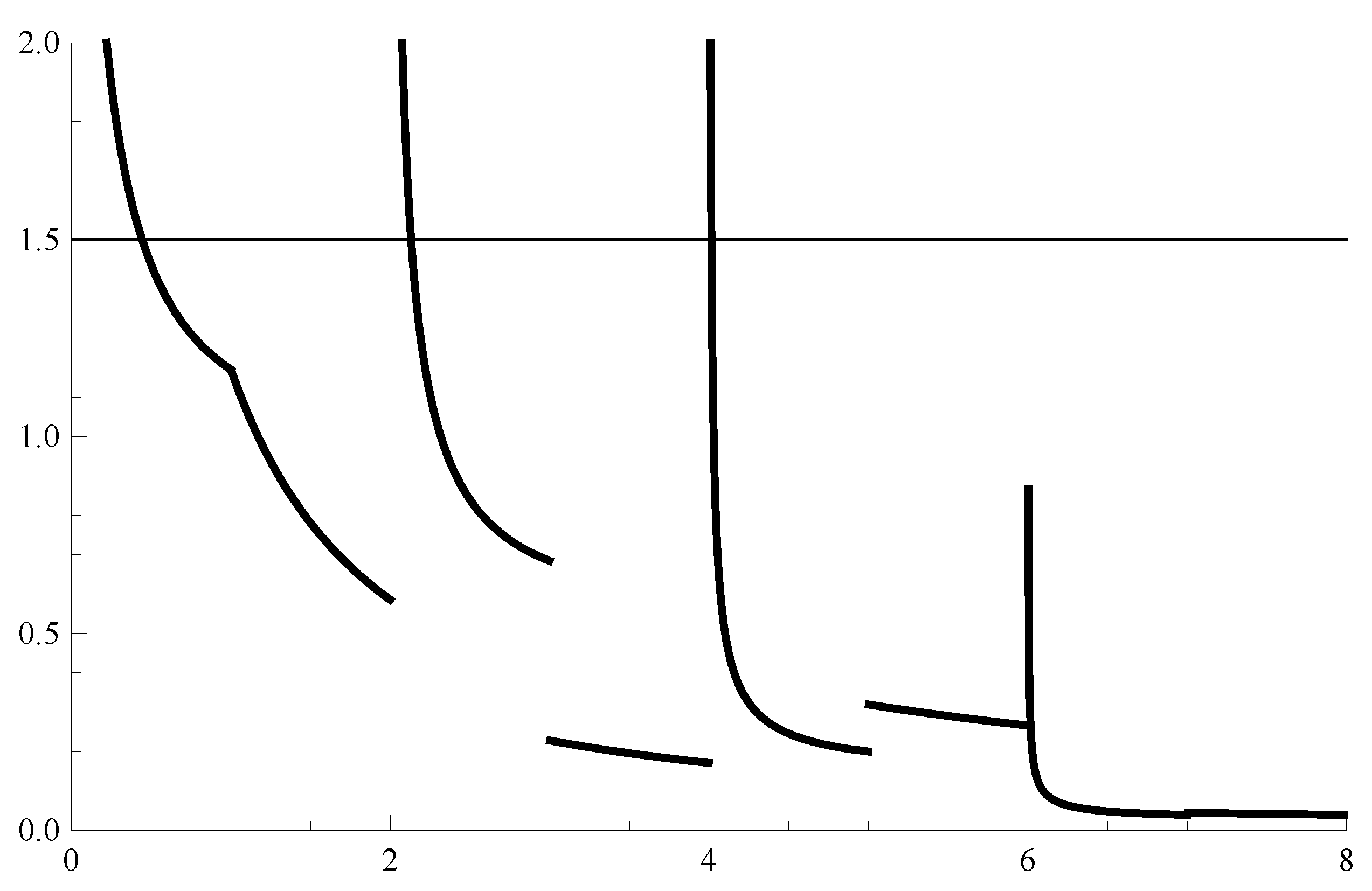
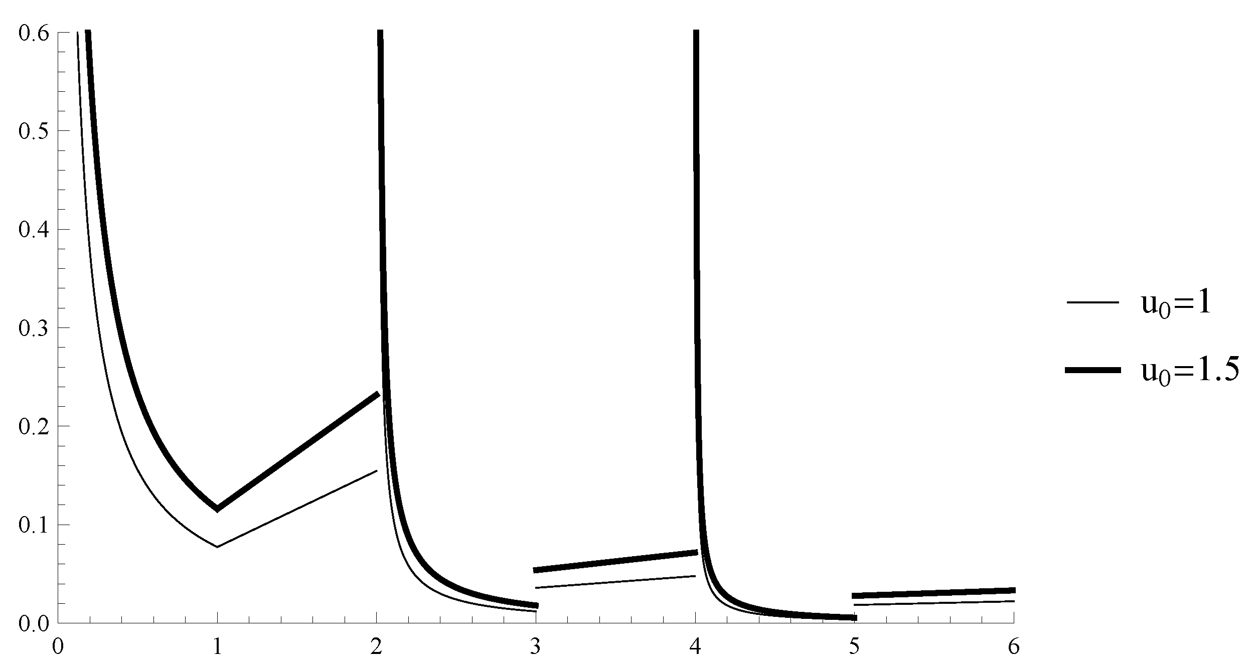
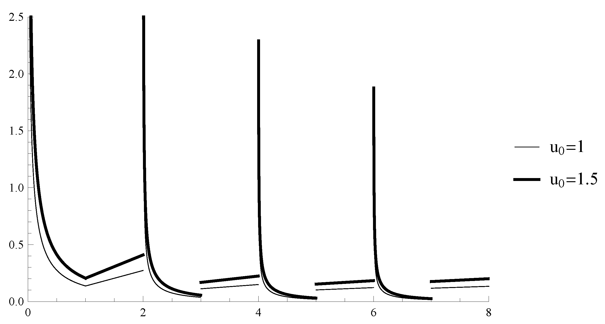
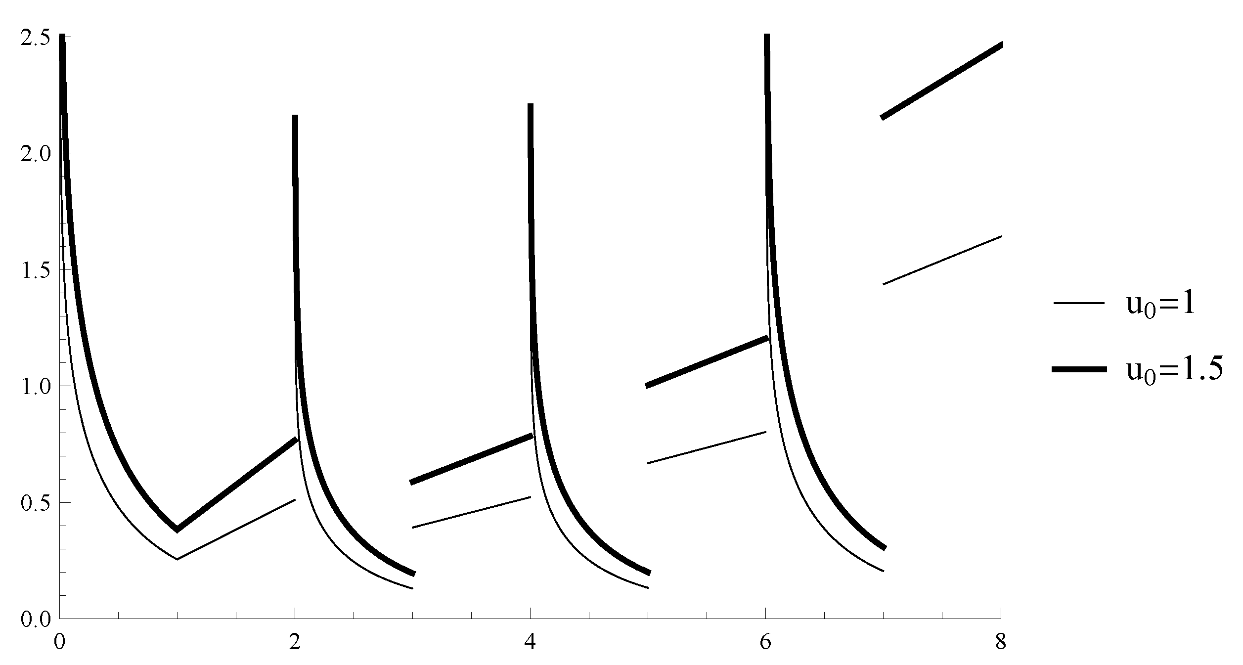
Example 1.

Consider the IVP for the scalar linear NIRLFDE

$$\begin{array}{cc}& {}_{t_i}^{RL}{D}_t^{q}y\left(t\right)=ay\left(t\right)fort\in (t_i,s_i],i=0,1,2,\dots ,\hfill \\ & \underset{t\to t_i+}{lim}\left[{(t-t_i)}^{1-q}y\left(t\right)\right]=\frac{y(s_{i-1}-0)}{t_i\Gamma \left(q\right)},fori=1,2,\dots ,\hfill \\ & y\left(t\right)=\frac{y(s_i-0)}{t}fort\in (s_i,t_{i+1}],i=0,1,2,\dots ,\hfill \\ & \underset{t\to 0+}{lim}\left[t^{1-q}y\left(t\right)\right]=\frac{y_0}{\Gamma \left(q\right)},\hfill \end{array}$$

(3)

where $y_0\in R$, $a\in R$.

The solution of Equation (3) is given by

$$y\left(t\right)=\left\{\begin{array}{cc}{y}_0\left(\prod _{i=0}^{k-1}\frac{{(s_i-t_i)}^{q-1}{E}_{q,q}\left(a{(s_i-t_i)}^q\right)}{t_{i+1}}\right){(t-t_k)}^{q-1}{E}_{q,q}\left(a{(t-t_k)}^q\right),\hfill & \mathrm{if}t\in (t_k,s_k],\hfill \\ y_0\left(\prod _{i=0}^{k-1}\frac{{(s_i-t_i)}^{q-1}{E}_{q,q}\left(a{(s_i-t_i)}^q\right)}{t_{i+1}}\right)\frac{{(s_k-t_k)}^{q-1}{E}_{q,q}\left(a{(s_k-t_k)}^q\right)}{t},\hfill & \mathrm{if}t\in (s_k,t_{k+1}],\hfill \\ \hfill & k=0,1,2,\dots .\hfill \end{array}\right.$$

It has singularities at the point $t_k,k=0,1,2,3,\dots$ which are the initial time and the end times of action of the non-instantaneous impulses at which the impulsive condition is switching to the differential equation (in the particular case $a=0.5,y_0=1$, $t_k=2k,s_k=k+1,k=0,1,2,\dots$, $q=0.3$ the graph of the solution $y\left(t\right)$ is given on Figure 1).

Figure 1. Example 1. Graph of the solution of Equation (3) for $a=0.5,y_0=1$, and $q=0.3$.

Example 1 illustrates that the stability of the solution for non-instantaneous impulsive differential equations in the case of the RL fractional derivative has to be studied on intervals excluding from the right the points $t_k,k=0,1,2,\dots$. In connection with this phenomenon we will define a new type of stability:

Definition 1.

The zero solution of the IVP for the NIRLFDE of Equation (1) is said to begeneralized Lipschitz stable in timeif there exist a nonegative integer N, positive numbers $\delta ,M:M\ge 1$ and a sequence of positive numbers ${\left\{T_i\right\}}_{i=0}^{\infty },T_i<{inf}_i(s_i-t_i)$ such that for any initial value $x_0\in {\mathbb{R}}^n:\left|\right|x_0\left|\right|<\delta$ the inequality $\left|\right|x(t;x_0)\left|\right|\le M\left|\right|x_0\left|\right|$ holds for $t\in {\cup }_{i=N}^{\infty }[t_i+T_i,t_{i+1}].$

Remark 9.

Note the generalized Lipschitz stability in time gives a bound of the solution to the right of an existing point and over intervals excluding to the right of any of the starting time points of the non-instantaneous impulses.

3. Lyapunov Functions and Comparison Results

Definition 2

([17]). Let $J\subset {\mathbb{R}}_{+},0\in J,$$\mathcal{J}=J\bigcap \left\{{\cup }_{i=0}^{\infty }(t_i,t_{i+1}]\right\}$ and $\Delta \subset {\mathbb{R}}^n$. We will say that the function $V(t,x)$ belongs to the class $\Lambda (J,\Delta )$ if $V\in C(\mathcal{J}\times \Delta ,{\mathbb{R}}_{+})$, $V(t_i,x)=V(t_i-0,x)={lim}_{\epsilon \to 0+}V(t_i-\epsilon ,x)$ for $i=1,2,\dots ,x\in \Delta$, and it is locally Lipschitz with respect to its second argument.

We will use two types of derivatives of Lyapunov functions from the class $\Lambda ({\mathbb{R}}_{+},\Delta )$ to study the Lipschitz stability of the NIRLFDE of Equation (1) (see Remark 1):

-

The RL fractional derivative of the Lyapunov function $V\in \Lambda ({\mathbb{R}}_{+},\Delta )$ among the NIRLFDE of Equation (1) is defined by

$${}_{t_k}^{RL}{D}^{q}V(t,x\left(t\right))=\frac{1}{\Gamma \left(1-q\right)}\frac{d}{ds}\underset{t_k}{\overset{t}{\int }}{\left(t-s\right)}^{-q}V(s,x\left(s\right))ds,t\in (t_k,s_k],k=0,1,2,\dots ,$$

(4)

where $x\in P{C}_{1-q}({\mathbb{R}}_{+},\Delta )$ is a solution of Equation (1).

-

The Dini fractional derivative of the Lyapunov function $V\in \Lambda ({\mathbb{R}}_{+},\Delta )$ among the NIRLFDE of Equation (1) is defined by:

$$\begin{array}{cc}& D_{\left(1\right)}^{t_k}V(t,x)=\underset{h\to 0+}{lim\; sup}\frac{1}{h^q}\left[V(t,x)-\sum _{r=1}^{\left[\frac{t-t_k}{h}\right]}{(-1)}^{r+1}{}_q{C}_{r}V(t-rh,x-h^{q}f(t,x))\right]\hfill \\ & \mathrm{for}t\in (t_k,s_k],x\in \Delta ,k=0,1,2,\dots .\hfill \end{array}$$

(5)

Remark 10.

The definition of the Dini fractional derivative of the Lyapunov function $V\in \Lambda ({\mathbb{R}}_{+},\Delta )$ among the NIRLFDE of Equation (1) is similar to the Grünwald–Letnikov fractional Dini derivative in Equation (2).

Remark 11.

Let $x\left(t\right)$ be a solution of Equation (1). Then for any $k=0,1,2,\dots$ the equality

$$\begin{array}{cc}\hfill D_{\left(1\right)}^{t_k}V(t,x\left(t\right))& =\underset{h\to 0+}{lim\; sup}\frac{1}{h^q}\left[V(t,x\left(t\right))-\sum _{r=1}^{\left[\frac{t-t_k}{h}\right]}{(-1)}^{r+1}{}_q{C}_{r}V(t-rh,x\left(t\right)-h^{q}f(t,x\left(t\right)))\right],\hfill \\ & t\in (t_k,s_k],\hfill \end{array}$$

holds.

We will use as a comparison scalar equation the following equation:

$$\begin{array}{cc}& {}_{t_i}^{RL}{D}_t^{q}u\left(t\right)=g(t,u\left(t\right))\mathrm{for}t\in (t_i,s_i],i=0,1,2,\dots ,\hfill \\ & \underset{t\to t_i+}{lim}\left[{(t-t_i)}^{1-q}u\left(t\right)\right]=\frac{H_{i-1}(t_i,u(s_{i-1}-0))}{\Gamma \left(q\right)},\mathrm{for}i=1,2,\dots ,\hfill \\ & u\left(t\right)=H_i(t,u(s_i-0))\mathrm{for}t\in (s_i,t_{i+1}],i=0,1,2,\dots ,\hfill \\ & \underset{t\to 0+}{lim}\left[t^{1-q}u\left(t\right)\right]=\frac{u_0}{\Gamma \left(q\right)},\hfill \end{array}$$

(6)

where $u_0\in \mathbb{R},g:{\cup }_{i=0}^{\infty }[t_i,s_i]\times \mathbb{R}\to \mathbb{R},H_i:[s_i,t_{i+1}]\times R\to R,i=0,1,2,\dots$.

We introduce the following conditions:

(A4) The function $g\in C({\cup }_{i=0}^{\infty }[t_i,s_i]\times \mathbb{R},\mathbb{R})$ is decreasing w.r.t. its second argument and $g(t,0)=0$ for $t\in {\cup }_{i=0}^{\infty }[t_i,s_i]$.

(A5) The functions $H_k\in C([s_k,t_{k+1}]\times \mathbb{R},\mathbb{R}),k=1,2,3,\dots ,$ are increasing w.r.t. its second argument and $H_k(t,0)=0$ for $t\in [s_k,t_{k+1}]$.

In our study we will use some comparison results with both defined above types of derivatives of Lyapunov functions.

3.1. Comparison Result with RL Fractional Derivative of Lyapunov Functions

Lemma 1.

Assume the following conditions are satisfied:

1. 

Conditions (A2)–(A5) are satisfied.

2. 

The function $x^{*}\left(t\right)=x(t;x_0),x^{*}\in P{C}_{1-q}({\mathbb{R}}_{+},{\mathbb{R}}^n)$ is a solution of Equation (1).

3. 

The function $u\left(t\right)=u(t;u_0),u\in P{C}_{1-q}({\mathbb{R}}_{+},\mathbb{R})$ is a solution of Equation (6).

4. 

The function $V\in \Lambda ({\mathbb{R}}_{+},{\mathbb{R}}^n)$ is such that

(i) 

The inequality

$${}_{t_i}^{RL}{D}_t^{q}V(t,x^{*}\left(t\right))\le g(t,V(t,x^{*}\left(t\right))),t\in (t_i,s_i],i=0,1,2,\dots ,$$

holds.

(ii) 

For all $i=0,1,2,\dots$ the inequalities

$$V(t,{\Psi }_i(t,x^{*}(s_i-0)))\le H_i(t,V(s_i,x^{*}(s_i-0))),t\in [s_i,t_{i+1}],$$

hold.

(iii) 

For all $i=1,2,\dots$ the inequalities

$$\underset{t\to t_i+}{lim}{(t-t_i)}^{1-q}V(t,x^{*}\left(t\right))\le \frac{V(t_i,x^{*}\left(t_i\right)))}{\Gamma \left(q\right)}$$

hold.

If ${lim}_{t\to 0+}{t}^{1-q}V(t,x^{*}\left(t\right))\le \frac{u_0}{\Gamma \left(q\right)},$ then the inequality

$$V(t,x^{*}\left(t\right))\le u\left(t\right)fort>0$$

(7)

holds.

Proof. 

Let $m\left(t\right)=V(t,x^{*}\left(t\right))$, $t>0$.

Case 1. Let $t\in (0,s_0]$.

Let $\epsilon >0$ be an arbitrary number. We will prove

$$m\left(t\right)<u\left(t\right)+t^{q-1}\epsilon ,t\in (0,s_0].$$

(8)

From the choice of the initial point $u_0$ we obtain

$$\begin{array}{cc}\hfill \underset{t\to 0+}{lim}{t}^{1-q}V(t,x^{*}\left(t\right))& \le \frac{u_0}{\Gamma \left(q\right)}<\frac{u_0}{\Gamma \left(q\right)}+\epsilon =\underset{t\to 0+}{lim}{t}^{1-q}u\left(t\right)+\underset{t\to 0+}{lim}{t}^{1-q}{t}^{q-1}\epsilon \hfill \\ & =\underset{t\to 0+}{lim}{t}^{1-q}\left(u\left(t\right)+t^{q-1}\epsilon \right).\hfill \end{array}$$

(9)

From inequalities (9) there exists a number $\delta >0$ such that $t^{1-q}V(t,x^{*}\left(t\right))<t^{1-q}\left(u\left(t\right)+t^{q-1}\epsilon \right)$ for $t\in (0,\delta )$, i.e., Equation (8) is satisfied on $(0,\delta )$.

If $\delta \ge s_0$ the inequality in Equation (8) is proved.

If $\delta <s_0$ we assume the inequality in Equation (8) is not true. Then there exists a point $t^{*}\in [\delta ,s_0]$ such that $m\left(t^{*}\right)=u\left(t^{*}\right)+{\left(t^{*}\right)}^{q-1}\epsilon ,m\left(t\right)<u\left(t\right)+t^{q-1}\epsilon ,t\in (0,t^{*})$.

From condition (A4), equality ${}_0^{RL}{D}_t^q{t}^{q-1}=0$ and Proposition 1 with $t_1=t^{*}$ and $v\left(t\right)=m\left(t\right)-u\left(t\right)-t^{q-1}\epsilon$ we obtain the inequality

$$\begin{array}{cc}\hfill {}_0^{RL}{D}_t^q{m\left(t\right)|}_{t=t^{*}}& \ge {}_0^{RL}{D}_t^q\left(u\left(t\right)+t^{q-1}\epsilon \right){{|}_{t=t^{*}}={}_0^{RL}{D}_t^{q}u\left(t\right)|}_{t=t^{*}}=g(t^{*},u\left(t^{*}\right))\hfill \\ & =g\left(t^{*},m\left(t^{*}\right)-{\left(t^{*}\right)}^{q-1}\epsilon \right)>g(t^{*},m\left(t^{*}\right)).\hfill \end{array}$$

(10)

The inequality of Equation (10) contradicts condition 4 (i). Therefore, the inequality in Equation (8) is true for any arbitrary number $\epsilon$ and thus Equation (7) holds for $t\in (0,s_0].$

Case 2. Let $t\in (s_0,t_1]$. Then from conditions 4(ii), (A5), and the inequality $V(s_0,x^{*}(s_0-0))\le u\left(s_0\right)$ we get $V(t,x^{*}\left(t\right))=V(t,{\Psi }_0(t,x^{*}(s_0-0))\le H_0(t,V(s_0,x^{*}(s_0-0)))\le H_0(t,u(s_0-0))=u\left(t\right)$, i.e., the inequality of Equation (7) holds on $(s_0,t_1]$.

Case 3. Let $t\in (t_1,s_1]$.

Let $\epsilon >0$ be an arbitrary number. We will prove

$$m\left(t\right)<u\left(t\right)+{(t-t_1)}^{q-1}\epsilon ,t\in (t_1,s_1].$$

(11)

From condition 4(iii) and the inequality $V(t_1,x^{*}\left(t_1\right))\le u\left(t_1\right)=H_0(t_1,u(s_0-0))$ we obtain

$$\begin{array}{cc}& \underset{t\to t_1+}{lim}{(t-t_1)}^{1-q}V(t,x^{*}\left(t\right))\le \frac{V(t_1,x^{*}\left(t_1\right))}{\Gamma \left(q\right)}\le \frac{H_0(t_1,u(s_0-0))}{\Gamma \left(q\right)}\hfill \\ & <\frac{H_0(t_1,u(s_0-0))}{\Gamma \left(q\right)}+\epsilon \hfill \\ & =\underset{t\to t_1+}{lim}\left[{(t-t_1)}^{1-q}u\left(t\right)\right]+\underset{t\to t_1+}{lim}{(t-t_1)}^{1-q}{(t-t_1)}^{q-1}\epsilon \hfill \\ & =\underset{t\to t_1+}{lim}{(t-t_1)}^{1-q}\left(u\left(t\right)+{(t-t_1)}^{q-1}\epsilon \right).\hfill \end{array}$$

(12)

From the inequality of Equation (12) there exists a number ${\delta }_1>0$ such that ${(t-t_1)}^{1-q}V(t,x^{*}\left(t\right))<{(t-t_1)}^{1-q}\left(u\left(t\right)+{(t-t_1)}^{q-1}\epsilon \right)$ for $t\in (t_1,t_1+{\delta }_1)$, i.e., inequality $V(t,x^{*}\left(t\right))<u\left(t\right)+{(t-t_1)}^{q-1}\epsilon$ holds, i.e., Equation (11) is satisfied on $(t_1,t_1+{\delta }_1)$.

If ${\delta }_1\ge s_1-t_1$ the inequality of Equation (11) is proved.

If ${\delta }_1<s_1-t_1$ we assume the inequality of Equation (11) is not true. Then there exists a point $t_1^{*}\in [t_1+\delta ,s_1]$ such that $m\left(t_1^{*}\right)=u\left(t_1^{*}\right)+{(t_1^{*}-t_1)}^{q-1}\epsilon ,m\left(t\right)<u\left(t\right)+{(t-t_1)}^{q-1}\epsilon ,t\in [t_1,t_1^{*})$.

From condition (A4), equality ${}_{t_1}^{RL}{D}_t^q{(t-t_1)}^{q-1}=0$ and Proposition 1 with $t_1=t_1^{*}$ and $v\left(t\right)=m\left(t\right)-u\left(t\right)-{(t-t_1)}^{q-1}\epsilon$ we obtain the inequality

$$\begin{array}{cc}\hfill {}_{t_1}^{RL}{D}_t^q{m\left(t\right)|}_{t=t_1^{*}}& \ge {}_{t_1}^{RL}{D}_t^q\left(u\left(t\right)+{(t-t_1)}^{q-1}\epsilon \right){{|}_{t=t_1^{*}}={}_{t_1}^{RL}{D}_t^{q}u\left(t\right)|}_{t=t_1^{*}}=g(t_1^{*},u\left(t_1^{*}\right))\hfill \\ & =g\left(t_1^{*},m\left(t_1^{*}\right)-{(t_1^{*}-t_1)}^{q-1}\epsilon \right)>g(t_1^{*},m\left(t_1^{*}\right)).\hfill \end{array}$$

(13)

The inequality of Equation (13) contradicts condition 4(i). Therefore, the inequality of Equation (11) is true for any arbitrary number $\epsilon$ and thus Equation (7) holds for $t\in (s_1,t_1].$

Following the above procedure we prove the claim of Lemma 1. □

3.2. Comparison Result with Dini Fractional Derivative of Lyapunov Functions

Lemma 2.

Assume:

1. 

Conditions 1,2,3, 4(ii) and 4(iii) of Lemma 1 are satisfied.

2. 

The function $V\in \Lambda ({\mathbb{R}}_{+},\mathbb{R})$ is such that the inequality

$$D_{\left(1\right)}^{t_k}V(t,x^{*}\left(t\right))\le g(t,V(t,x^{*}\left(t\right)),fort\in (t_k,s_k],k=0,1,2,\dots ,$$

holds.

If ${lim}_{t\to 0+}{t}^{1-q}V(t,x^{*}\left(t\right))\le \frac{u_0}{\Gamma \left(q\right)},$ then the inequality $V(t,x^{*}\left(t\right))\le u\left(t\right)$ for $t>0$ holds.

Proof. 

The proof is similar to the one in Lemma 1 where instead of the RL fractional derivative of the Lyapunov function we will use the Dini fractional derivative. The main difference between both proofs of Lemma 1 and Lemma 2, respectively, is connected with the inequalities of Equations (10) and (13) for $t^{*}\in (t_0,s_0]$ and $t_1^{*}\in (t_1,s_1]$.

We will consider the general case of $(t_k,s_k],k=0,1,2,\dots$, i.e., assume that for a fixed non-zero integer k there exist ${\delta }_k\in (0,t_k-s_k)$ and a point $t_k^{*}\in (t_k+{\delta }_k,s_k]$ such that $m\left(t_k^{*}\right)=u\left(t_k^{*}\right)+{(t_k^{*}-t_k)}^{q-1}\epsilon ,m\left(t\right)<u\left(t\right)+{(t-t_k)}^{q-1}\epsilon ,t\in (t_k,t_k^{*})$.

According to Remark 6 with $\tau =t_k^{*}$ we obtain the inequality

$$\begin{array}{cc}\hfill {}_{t_k}^{GL}{D}_{+}^q{m\left(t\right)|}_{t=t_k^{*}}& \ge {}_{t_k}^{GL}{D}_{+}^q{u\left(t\right)|}_{t=t_k^{*}}+{}_0^{GL}{D}_{+}^q\left({(t-t_k)}^{q-1}\epsilon \right){{|}_{t=t_k^{*}}={}_{t_k}^{GL}{D}_{+}^{q}u\left(t\right)|}_{t=t_k^{*}}\hfill \\ & =g(t_k^{*},u\left(t_k^{*}\right))=g(t_k^{*},m\left(t_k^{*}\right)-{(t_k^{*}-t_k)}^{q-1}\epsilon )>g(t_k^{*},m\left(t_k^{*}\right)).\hfill \end{array}$$

(14)

For any fixed $t\in (t_k,s_k]$ we have (see Equation (2))

$$\begin{array}{cc}& {}_{t_k}^{GL}{D}_{+}^{q}m\left(t\right)=\underset{h\to 0+}{lim\; sup}\frac{1}{h^q}\sum _{r=0}^{\left[\frac{t-t_k}{h}\right]}{(-1)}^r{}_q{C}_{r}m(t-rh)\hfill \\ & =\underset{h\to 0+}{lim\; sup}\frac{1}{h^q}\sum _{r=0}^{\left[\frac{t-t_k}{h}\right]}{(-1)}^r{}_q{C}_{r}V(t-rh,x^{*}(t-rh))\hfill \\ & =\underset{h\to 0+}{lim\; sup}\frac{1}{h^q}\left\{V(t,x^{*}\left(t\right))-\sum _{r=1}^{\left[\frac{t-t_k}{h}\right]}{(-1)}^{r+1}{}_q{C}_{r}V(t-rh,x^{*}(t-rh))\right]\hfill \\ & =\underset{h\to 0+}{lim\; sup}\frac{1}{h^q}\left[V(t,x^{*}\left(t\right))-\sum _{r=1}^{\left[\frac{t-t_k}{h}\right]}{(-1)}^{r+1}{}_q{C}_{r}V(t-rh,x^{*}\left(t\right)-h^{q}f(t,x^{*}\left(t\right))\right]\hfill \\ & +\sum _{r=1}^{\left[\frac{t-t_k}{h}\right]}{(-1)}^{r+1}{}_q{C}_r\left[V(t-rh,x^{*}\left(t\right)-h^{q}f(t,x^{*}\left(t\right))-V(t-rh,x^{*}(t-rh))\right]\}.\hfill \end{array}$$

(15)

Denote

$$F(t,x^{*},t_k,h)=\sum _{r=1}^{\left[\frac{t-t_k}{h}\right]}{(-1)}^{r+1}{}_q{C}_r{x}^{*}(t-rh).$$

From Equation (1) it follows

$${}_{t_k}^{GL}{D}_t^q{x}^{*}\left(t\right)=\underset{h\to 0+}{lim\; sup}\left[x^{*}\left(t\right)-F(t,x^{*},t_k,h)\right]={}_{t_k}^{RL}{D}_t^q{x}^{*}\left(t\right)=f(t,x^{*}\left(t\right)).$$

Therefore, $x^{*}\left(t\right)-h^{q}f(t,x^{*}\left(t\right))=F(t,x^{*},t_k,h)+\Omega \left(h^q\right)$ where ${lim}_{h\to 0+}\frac{\left|\right|\Omega \left(h^q\right)\left|\right|}{h^q}=0$.

Therefore, for any $r=1,2,\dots$ and $h>0$

$$\begin{array}{cc}& V(t-rh,x^{*}\left(t\right)-h^{q}f(t,x^{*}\left(t\right))-V(t-rh,x^{*}(t-rh))\hfill \\ & \le L\left|\right|F(t,x^{*},t_k,h)+\Omega \left(h^q\right)-x^{*}(t-rh)\left|\right|\hfill \\ & \le L\left|\right|\sum _{j=1}^{\left[\frac{t-t_k}{h}\right]}{(-1)}^{j+1}{}_q{C}_j{x}^{*}(t-jh)-x^{*}(t-rh)\left|\right|+L\left|\right|\Omega \left(h^q\right)\left|\right|.\hfill \end{array}$$

(16)

Thus, by ${(1+u)}^{\alpha }=1+{\sum }_{k=1}^{\infty }{}_{\alpha }{C}_k{u}^k$, i.e., $1={\sum }_{k=1}^{\infty }{(-1)}^{k+1}{}_{\alpha }{C}_k$, we obtain

$$\begin{array}{cc}& \left|\right|\sum _{j=1}^{\left[\frac{t-t_k}{h}\right]}{(-1)}^{j+1}{}_q{C}_j{x}^{*}(t-jh)-x^{*}(t-rh)\left|\right|\hfill \\ & =\left|\right|\sum _{j=1}^{\left[\frac{t-t_k}{h}\right]}{(-1)}^{j+1}{}_q{C}_j{x}^{*}(t-jh)-\left(\sum _{j=1}^{\infty }{(-1)}^{j+1}{}_q{C}_j\right)x^{*}(t-rh)\left)\right||\hfill \\ & \le \left|\right|\sum _{j=1}^{\left[\frac{t-t_k}{h}\right]}{(-1)}^{j+1}{}_q{C}_j[x^{*}(t-jh)-x^{*}(t-rh)]\left|\right|\hfill \\ & +\left|\right|\sum _{j=\left[\frac{t-t_k}{h}\right]}^{\infty }{(-1)}^{j+1}{}_q{C}_j\left|\right|\left|\right|x^{*}(t-rh)\left|\right|.\hfill \end{array}$$

(17)

From Equations (15)–(17) and condition 2 of Lemma 2 we get

$$\begin{array}{cc}& {}_{t_k}^{GL}{D}_{+}^{q}m\left(t\right)\le D_{\left(1\right)}^{t_k}V(t,x^{*}\left(t\right))+L\underset{h\to 0+}{lim\; sup}\frac{\left|\right|\Omega \left(h^q\right)\left|\right|}{h^q}\sum _{r=1}^{\left[\frac{t-t_k}{h}\right]}{(-1)}^{r+1}{}_q{C}_r\hfill \\ & +L\underset{h\to 0+}{lim\; sup}\frac{1}{h^q}\sum _{r=1}^{\left[\frac{t-t_k}{h}\right]}{(-1)}^{r+1}{}_q{C}_r\left|\right|\sum _{j=1}^{\left[\frac{t-t_k}{h}\right]}{(-1)}^{j+1}{}_q{C}_j{x}^{*}(t-jh)-x^{*}(t-rh)\left|\right|\hfill \\ & =D_{\left(1\right)}^{t_k}V(t,x^{*}\left(t\right))\hfill \\ & +L\underset{h\to 0+}{lim\; sup}\frac{1}{h^q}\sum _{r=1}^{\left[\frac{t-t_k}{h}\right]}{(-1)}^{r+1}{}_q{C}_r\left|\right|\sum _{j=1}^{\left[\frac{t-t_k}{h}\right]}{(-1)}^{j+1}{}_q{C}_j[x^{*}(t-jh)-x^{*}(t-rh)]\left|\right|\hfill \\ & +L\underset{h\to 0+}{lim\; sup}\left|\right|\sum _{j=\left[\frac{t-t_k}{h}\right]}^{\infty }{(-1)}^{j+1}{}_q{C}_j\left|\right|\frac{1}{h^q}\sum _{r=1}^{\left[\frac{t-t_k}{h}\right]}{(-1)}^{r+1}{}_q{C}_r\left|\right|x^{*}(t-rh)\left|\right|\hfill \\ & =D_{\left(1\right)}^{t_k}V(t,x^{*}\left(t\right))\le g(t,V(t,x^{*}\left(t\right))).\hfill \end{array}$$

(18)

The inequality of Equation (18) contradicts the inequality of Equation (14). □

4. Main Results

We will obtain some sufficient conditions for generalized Lipschitz stability in time by Lyapunov functions and their two fractional derivatives.

4.1. RL Fractional Derivative of Lyapunov Functions Among the Solutions

Theorem 1.

Let the following conditions be satisfied:

1. 

Conditions (A1)–(A5) are fulfilled.

2. 

There exists a function $V\in \Lambda ({\mathbb{R}}_{+},{\mathbb{R}}^n)$ such that

(i) 

there exists a sequence of numbers ${\left\{{\tau }_i\right\}}_{i=0}^{\infty },0<{\tau }_i<\lambda ={inf}_i(s_i-t_i)$ such that the inequality

$$b\left(\right|\left|x\right|\left|\right)\le V(t,x),x\in {\mathbb{R}}^n,t\in {\cup }_{i=0}^{\infty }[t_i+{\tau }_i,t_{i+1}]$$

(19)

holds, where $b\in \mathit{M}\left(\right[0,\rho \left]\right)$, $\rho >0$;

(ii) 

for any function $y\in C_{1-q}([0,s_0],{\mathbb{R}}^n):{lim}_{t\to 0+}\left(t^{1-q}y\left(t\right)\right)=y_0\in S_{\rho }$ the inequality

$$t^{1-q}{V(t,y\left(t\right))|}_{t=0+}=\underset{t\to 0+}{lim}{t}^{1-q}V(t,y\left(t\right))\le a\left(\right||y_0\left|\right|)$$

holds with $a\in \mathit{K}\left(\right[0,\rho \left]\right)$;

(iii) 

For all $i=0,1,2,\dots$ the inequalities

$$V(t,{\Psi }_i(t,x))\le H_i(t,V(s_i,x)),t\in (s_i,t_{i+1}],x\in {\mathbb{R}}^n,$$

hold;

(iv) 

for any function $y\in C_{1-q}([t_k,s_k],{\mathbb{R}}^n):{lim}_{t\to t_k+}\left({(t-t_k)}^{1-q}y\left(t\right)\right)=\frac{y_k}{\Gamma \left(q\right)}<\infty$ the inequality

$${(t-t_k)}^{1-q}V(t,y\left(t\right)){|}_{t=t_k+}=\underset{t\to t_k+}{lim}{(t-t_k)}^{1-q}V(t,y\left(t\right))\le V(t_k,y_k)$$

holds;

(v) 

for any initial value $x_0\in S_{\rho }$ and the corresponding solution $x\left(t\right)=x(t;x_0)$ of Equation (1) the inequality

$${}_{t_k}^{RL}{D}_t^{q}V(t,x\left(t\right))\le g(t,V(t,x\left(t\right))),t\in (t_k,s_k],k=0,1,2,\dots ,$$

holds.

3.

The zero solution of the scalar comparison Equation (6) is generalized Lipschitz stable in time.

Then the zero solution of the system in Equation (1) is generalized Lipschitz stable in time.

Proof. 

Let the zero solution of Equation (6) be generalized Lipschitz stable in time. Therefore, there exist a nonegative integer N, a sequence of numbers ${\left\{{\varsigma }_i\right\}}_{i=0}^{\infty },{\varsigma }_i\in (0,\delta ),0<\delta <\lambda ={inf}_i(s_i-t_i)$, a number ${\delta }_1>0$, and $M_1\ge 1$ such that for any for $u_0\in {\mathbb{R}}^n:\left|u_0\right|<{\delta }_1$ the inequality

$$|u(t;u_0)|\le M_1\left|u_0\right|\mathrm{for}t\in {\cup }_{i=N}^{\infty }[t_i+{\varsigma }_i,t_{i+1}]$$

(20)

holds, where $u(t;u_0)$ is a solution of Equation (6) with the initial value $u_0$.

From the inclusions $a\in \mathit{K}\left(\right[0,\rho \left]\right)$ and $b\in \mathit{M}\left(\right[0,\rho \left]\right)$ there exists a function $q_b\left(u\right)\ge 1$ for $\alpha \ge 1$ and a positive constant $K_a$ such that

$$\alpha r\le b\left(r{q}_a\left(\alpha \right)\right),r\in [0,\rho ],$$

(21)

and

$$a\left(r\right)\le K_{a}r,r\in [0,\rho ].$$

(22)

Without loss of generality we can assume $K_a\ge 1$.

Choose the positive constants $M_2,\delta$ such that $M_2>max\{1,q_b\left(M_1{K}_a\right)\}\ge 1$ and $\delta =min\left\{\rho ,\frac{{\delta }_1}{K_a}\right\}$. Choose the initial value $x_0\in {\mathbb{R}}^n:\left|\right|x_0\left|\right|<\delta$, thus $x_0\in S_{\rho }$.

Consider the solution $x^{*}\left(t\right)=x(t;x_0)$ of Equation (1) for the chosen initial value $x_0$. Then applying $\Gamma \left(q\right)>1$ for $q\in (0,1)$ we obtain $\left|\right|{lim}_{t\to 0+}{t}^{1-q}{x}^{*}\left(t\right)\left|\right|=\left|\right|\frac{x_0}{\Gamma \left(q\right)}\left|\right|<\frac{\delta }{\Gamma \left(q\right)}<\delta \le \rho$, i.e., ${lim}_{t\to 0+}{t}^{1-q}{x}^{*}\left(t\right)\in S_{\rho }$ and according to condition 2(ii) the inequalities

$$t^{1-q}V(t,x^{*}\left(t\right)){|}_{t=0+}<a\left(\frac{\left|\right|x_0\left|\right|}{\Gamma \left(q\right)}\right)<a\left(\right||x_0\left|\right|)$$

(23)

hold.

Consider the solution $u^{*}\left(t\right)$ of Equation (6) with $u_0^{*}={lim}_{t\to 0+}{t}^{1-q}V(t,x^{*}\left(t\right))$. From the choice of $x_0$, the inequalities of Equations (22) and (23) and condition $2\left(ii\right)$ we obtain $u_0^{*}={lim}_{t\to 0+}{t}^{1-q}V(t,x^{*}\left(t\right))\le a\left(\frac{\left|\right|x_0\left|\right|}{\Gamma \left(q\right)}\right)<a\left(\right||x_0\left|\right|)\le K_a\left|\right|x_0\left|\right|<K_a\delta \le {\delta }_1$. Therefore, the function $u^{*}\left(t\right)$ satisfies Equation (20) for ${\cup }_{i=N}^{\infty }[t_i+{\varsigma }_i,t_{i+1}]$ with $u_0=u_0^{*}$, where $u^{*}\left(t\right)=u(t;u_0^{*})$ is a solution of Equation (6) with the initial value $u_0^{*}$.

From condition 2(v) of Theorem 1 for $x\left(t\right)\equiv x^{*}\left(t\right)$ we have condition 4(i) of Lemma 1.

From condition 2(iii) of Theorem 1 for $x=x^{*}(s_i-0)$ we have condition 4(ii) of Lemma 1.

From condition 2(iv) of Theorem 1 for $y\left(t\right)\equiv x^{*}\left(t\right)$ and $y_k=x^{*}(t_i-0)$ we have condition 4(iii) of Lemma 1.

Therefore, all conditions of Lemma 1 are satisfied and thus,

$$V(t,x^{*}\left(t\right))\le u^{*}\left(t\right)\mathrm{for}t>0.$$

(24)

Let $T_i=max\{{\tau }_i,{\varsigma }_i\}$ for $i=0,1,2,\dots$. Then for any $k=0,1,2,\dots$ the inclusions $[t_k+T_k,t_{k+1}]\subset [t_k+{\tau }_k,t_{k+1}]$ and $[t_k+T_k,t_{k+1}]\subset [t_k+{\varsigma }_k,t_{k+1}]$ hold.

Let $k\ge N$ be a fixed integer. Then from conditions 2(i), 2(ii), the inequalities of Equations (20)–(22) with $r=\left|\right|x_0\left|\right|$, $\alpha =M_1{K}_a>1$ and Equations (23) and (24) we obtain for $t\in [t_k+T_k,t_{k+1}]$

$$\begin{array}{cc}\hfill b\left(\right|\left|x^{*}\left(t\right)\right|\left|\right)& \le V(t,x^{*}\left(t\right))\le u^{*}\left(t\right)<M_1|u_0^{*}|=M_1{t}^{1-q}V(t,x^{*}\left(t\right)){|}_{t=0+}<M_{1}a\left(\right||x_0\left|\right|)\hfill \\ & \le M_1{K}_a\left|\right|x_0\left|\right|\le b(q_b\left(M_1{K}_a\right)\left|\right|x_0\left|\right|)\le b(M_2\left|\right|x_0\left|\right|).\hfill \end{array}$$

(25)

The inequality in Equation (25) proves the claim of Theorem 1. □

Theorem 2.

Let the conditions of Theorem 1 be satisfied where$a\left(s\right)=A_2{s}^p,A_2>0,p\ge 1$in condition 2(ii) and the condition 2(i) is replaced by:

${\mathit{2}}^{*}\left(\mathit{i}\right)$there exists a sequence of numbers${\left\{{\tau }_i\right\}}_{i=0}^{\infty },0<{\tau }_i<\lambda ={inf}_i(s_i-t_i)$such that the inequality

$${\mu \left(t\right)\left|\right|x\left|\right|}^p\le V(t,x),x\in {\mathbb{R}}^n,t\in {\cup }_{i=0}^{\infty }[t_i+{\tau }_i,t_{i+1}],$$

(26)

holds where $\mu \left(t\right)\ge A_1,t\in {\cup }_{i=0}^{\infty }[t_i+{\tau }_i,t_{i+1}]$, $A_1>0$ is a constant.

Then the zero solution of the system in Equation (1) is generalized Lipschitz stable in time.

Proof. 

The proof is similar to the one in Theorem 1 where $M_2=\sqrt[p]{\frac{M_1{A}_2}{A_1}}$ and $\delta =min\left\{\lambda ,\sqrt[p]{\frac{{\delta }_1}{A_2}}\right\}$. □

4.2. Dini Fractional Derivative of Lyapunov Functions Among the Solutions

Theorem 3.

Let the conditions of Theorem 1 be satisfied where condition 2(v) is replaced by:

2(v*) the inequality

$$D_{\left(1\right)}^{t_k}V(t,x)\le g(t,V(t,x)),x\in {\mathbb{R}}^n,t\in (t_k,s_k],k=0,1,2,\dots ,$$

holds.

Then the zero solution of Equation (1) is generalized Lipschitz stable in time.

The proof of Theorem 3 is similar to the one of Theorem 1 where Lemma 2 is applied instead of Lemma 1.

Theorem 4.

Let the conditions of Theorem 1 be satisfied where $a\left(s\right)=A_2{s}^p,A_2>0,p\ge 1$ in condition 2(ii), the condition 2(i) is replaced by condition 2*(i) of Theorem 2 and the condition 2(v) is replaced by condition 2(v*) of Theorem 3.

Then the zero solution of Equation (1) is generalized Lipschitz stable in time.

The proof of Theorem 4 is similar to the one of Theorem 2 with the application of Lemma 2 so we omit it.

Example 2.

Let the sequences ${\left\{t_i\right\}}_{i=0}^{\infty }$, $t_0=0$, and ${\left\{s_i\right\}}_{i=0}^{\infty }$ be given such that ${sup}_k(t_{k+1}-t_k)=L\ge 1$. Consider IVP for the system of non-instantaneous impulsive RL fractional differential equations

$$\begin{array}{cc}& {}_{t_k}^{RL}{D}_t^q{x}_1\left(t\right)=-\left(0.5t^{q-1}+t^{-q}\frac{\Gamma (2-q)}{\Gamma (2-2q)}+x_2^2\left(t\right)\right)x_1\left(t\right),\hfill \\ & {}_{t_k}^{RL}{D}_t^q{x}_2\left(t\right)=-\left(0.5t^{q-1}+t^{-q}\frac{\Gamma (2-q)}{\Gamma (2-2q)}-\frac{x_1^2\left(t\right)}{1+x_2^2\left(t\right)}\right)x_2\left(t\right)\hfill \\ & fort\in (t_k,s_k],k=0,1,2,\dots ,\hfill \\ & x_1\left(t\right)={\Psi }_k^1(t,x_1(s_k-0),x_2(s_k-0)),\hfill \\ & x_2\left(t\right)={\Psi }_k^2(t,x_1(s_k-0),x_2(s_k-0)),fort\in (s_k,t_{k+1}],k=0,1,2,\dots ,\hfill \\ & \underset{t\to t_k+}{lim}\left[{(t-t_k)}^{1-q}{x}_1\left(t\right)\right]=\frac{{\Psi }_{k-1}^1(t_k,x_1(s_{k-1}-0),x_2(s_{k-1}-0))}{\Gamma \left(q\right)},\hfill \\ & \underset{t\to t_k+}{lim}\left[{(t-t_k)}^{1-q}{x}_2\left(t\right)\right]=\frac{{\Psi }_{k-1}^2(t_k,x_1(s_{k-1}-0),x_2(s_{k-1}-0))}{\Gamma \left(q\right)},k=1,2,\dots ,\hfill \\ & \underset{t\to t_0+}{lim}\left[t^{1-q}{x}_1\left(t\right)\right]=\frac{x_{0,1}}{\Gamma \left(q\right)},\underset{t\to t_0+}{lim}\left[t^{1-q}{x}_2\left(t\right)\right]=\frac{x_{0,2}}{\Gamma \left(q\right)},\hfill \end{array}$$

(27)

where $x\in R^2,x=(x_1,x_2)$, ${\Psi }_k^1(t,x_1,x_2)=\frac{x_1}{t},{\Psi }_k^2(t,x_1,x_2)=\frac{x_2}{t}$ for $t\in [s_k,t_{k+1}],k=0,1,2,\dots .$

Consider the Lyapunov function $V(t,x)={(t-t_k)}^{1-q}(x_1^2+x_2^2)$ for $t\in (t_k,t_{k+1}],k=0,1,2,\dots ,$ and $x=(x_1,x_2)\in {\mathbb{R}}^2$. The function $V\in \Lambda ([0,\infty ),R^2)$ is locally Lipschitz with a constant L.

Thus, condition 2*(i) of Theorem 2 is satisfied with $p=2,\mu \left(t\right)={(t-t_k)}^{1-q}$ for $t\in (t_k,t_{k+1})$ and ${\tau }_k:{\tau }_k=t_k+\sqrt[1-q]{0.1},A_1=\sqrt[1-q]{0.1}$.

Let the function $y\in C_{1-q}([0,s_0],{\mathbb{R}}^2)$, $y=(y_1,y_2)$, be such that ${lim}_{t\to 0+}\left(t^{1-q}{y}_k\left(t\right)\right)=y_{0,k},k=1,2$. Then

$$\begin{array}{cc}& \underset{t\to 0+}{lim}{t}^{1-q}V(t,y\left(t\right))=\underset{t\to 0+}{lim}{t}^{1-q}\left(t^{1-q}(y_1^2\left(t\right)+y_2^2\left(t\right)\right)\hfill \\ & ={\left(\underset{t\to 0+}{lim}{t}^{1-q}{y}_1\left(t\right)\right)}^2+{\left(\underset{t\to 0+}{lim}{t}^{1-q}{y}_2\left(t\right)\right)}^2=y_{0,1}^2+y_{0,2}^2=\left|\right|y_0{\left|\right|}^2.\hfill \end{array}$$

(28)

Therefore, condition 2(ii) of Theorem 1 is satisfied with $a\left(s\right)=A_2{s}^p,A_2=1,p=2$.

Let the function $y\in C_{1-q}([t_k,s_k],{\mathbb{R}}^2):{lim}_{t\to t_k+}\left({(t-t_k)}^{1-q}y\left(t\right)\right)=\frac{y_k}{\Gamma \left(q\right)}<\infty ,y_k=(y_{1,k},y_{2,k})$. Then for $t\in (t_k,t_{k+1}]$ we obtain the inequality

$$\begin{array}{cc}& {(t-t_k)}^{1-q}V(t,y\left(t\right)){|}_{t=t_k+}=\underset{t\to t_k+}{lim}{(t-t_k)}^{1-q}V(t,y\left(t\right))\hfill \\ & =\underset{t\to t_k+}{lim}{(t-t_k)}^{1-q}{(t-t_k)}^{1-q}(y_1{\left(t\right)}^2+y_2{\left(t\right)}^2)\hfill \\ & ={\left(\underset{t\to t_k+}{lim}{(t-t_k)}^{1-q}{y}_1\left(t\right)\right)}^2+{\left(\underset{t\to t_k+}{lim}{(t-t_k)}^{1-q}{y}_2\left(t\right)\right)}^2<y_{1,k}^2+y_{2,k}^2\hfill \\ & \le {(t_k-t_{k-1})}^{1-q}(y_{1,k}^2+y_{2,k}^2)=V(t_k,y_k).\hfill \end{array}$$

(29)

Therefore, condition 2(iv) of Theorem 1 is satisfied.

Let k be a fixed non-negative integer and $t\in [s_i,t_{i+1}],x\in {\mathbb{R}}^2,x=(x_1,x_2)$. Then we obtain the inequalities

$$\begin{array}{cc}\hfill V(t,{\Psi }_i(t,x^{*}(s_i-0)))& ={(t-t_i)}^{1-q}\left(\frac{x_1^2}{t^2}+\frac{x_2^2}{t^2}\right)=H_i(t,V(s_i,x^{*}(s_i-0))),\hfill \end{array}$$

(30)

Therefore, condition 2(iii) of Theorem 1 is satisfied with $H_i(t,u)=\frac{u}{t^2}$. The RL fractional derivative of the Lyapunov function, i.e., ${}_{t_k}^{RL}{D}_t^{q}V(t,x\left(t\right))={}_{t_k}^{RL}{D}_t^q{(t-t_k)}^{1-q}(x_1^2\left(t\right)+x_2^2\left(t\right))=\frac{1}{\Gamma \left(1-q\right)}\frac{d}{dt}\underset{a}{\overset{t}{\int }}{\left(t-s\right)}^{-q}{(s-t_k)}^{1-q}(x_1^2\left(s\right)+x_2^2\left(s\right))ds$ with $x\left(t\right)=(x_1\left(t\right),x_2\left(t\right)),t>0$ being the solution of Equation (27), is very difficult to obtain, so the results with the RL fractional derivative of Lyapunov functions are not applicable.

We will apply the Dini fractional derivative of the function V among Equation (27).

Let k be a fixed non-negative integer and $t\in (t_k,s_k],x_1,x_2\in \mathbb{R}$. Then we get

$$\begin{array}{cc}& D_{\left(27\right)}^{t_k}{(t-t_k)}^{1-q}(x_1^2+x_2^2)=\underset{h\to 0+}{lim\; sup}\frac{1}{h^q}[{(t-t_k)}^{1-q}(x_1^2+x_2^2)\hfill \\ & -\sum _{r=1}^{\left[\frac{t-t_k}{h}\right]}{(-1)}^{r+1}{}_q{C}_r{(t-rh-t_k)}^{1-q}[{(x_1-h^q{f}_1(t,x))}^2+{(x_2-h^q{f}_2(t,x))}^2]]\hfill \\ & =\underset{h\to 0+}{lim\; sup}\frac{1}{h^q}{(t-t_k)}^{1-q}\left[x_1^2-{(x_1-h^q{f}_1(t,x))}^2+x_2^2-{(x_2-h^q{f}_2(t,x))}^2\right]\hfill \\ & +\underset{h\to 0+}{lim\; sup}\frac{1}{h^q}[{(x_1-h^q{f}_1(t,x))}^2+{(x_2-h^q{f}_2(t,x))}^2]\sum _{r=0}^{\left[\frac{t-t_k}{h}\right]}{(-1)}^r{}_q{C}_r{(t-t_k-rh)}^{1-q}\hfill \\ & =\underset{h\to 0+}{lim\; sup}\frac{1}{h^q}{(t-t_k)}^{1-q}\left[(2x_1-h^q{f}_1(t,x))h^q{f}_1(t,x)+2(x_2+h^q{f}_2(t,x))h^q{f}_2(t,x)\right]\hfill \\ & +[x_1^2+x_2^2]{}_{t_k}^{RL}{D}_t^q{(t-t_k)}^{1-q}\hfill \\ & =2{(t-t_k)}^{1-q}{x}_1{f}_1(t,x)+2{(t-t_k)}^{1-q}{x}_2{f}_2(t,x)+[x_1^2+x_2^2]\frac{\Gamma (2-q)}{\Gamma (2-2q)}{(t-t_k)}^{1-2q}\hfill \\ & =2{(t-t_k)}^{1-q}{x}_1(-0.5t^{q-1}{x}_1-t^{-q}\frac{\Gamma (2-q)}{\Gamma (2-2q)}{x}_1-x_2^2{x}_1)\hfill \\ & +2{(t-t_k)}^{1-q}{x}_2(-0.5t^{q-1}{x}_2-t^{-q}\frac{\Gamma (2-q)}{\Gamma (2-2q)}{x}_2+\frac{x_2{x}_1^2}{1+x_2^2})\hfill \\ & +[x_1^2+x_2^2]\frac{\Gamma (2-q)}{\Gamma (2-2q)}{(t-t_k)}^{1-2q}\hfill \\ & \le 2{(t-t_k)}^{1-q}{x}_1(-0.5t^{q-1}{x}_1-{(t-t_k)}^{-q}\frac{\Gamma (2-q)}{\Gamma (2-2q)}{x}_1-x_2^2{x}_1)\hfill \\ & +2{(t-t_k)}^{1-q}{x}_2(-0.5t^{q-1}{x}_2-t^{-q}\frac{\Gamma (2-q)}{\Gamma (2-2q)}{x}_2+\frac{x_2{x}_1^2}{1+x_2^2})\hfill \\ & +[x_1^2+x_2^2]\frac{\Gamma (2-q)}{\Gamma (2-2q)}{(t-t_k)}^{1-2q}=-V(t,x)-[x_1^2+x_2^2]\frac{\Gamma (2-q)}{\Gamma (2-2q)}{(t-t_k)}^{1-2q}\hfill \\ & \le -V(t,x)fort>0,x\in {\mathbb{R}}^2.\hfill \end{array}$$

(31)

Therefore, condition 2(v*) of Theorem 3 is satisfied with $g(t,u)\equiv -u,u\in \mathbb{R}$.

Consider the IVP for the scalar linear NIRLFDE

$$\begin{array}{cc}& {}_{t_i}^{RL}{D}_t^{q}u\left(t\right)=-u\left(t\right)fort\in (t_i,s_i],i=0,1,2,\dots ,\hfill \\ & \underset{t\to t_i+}{lim}\left[{(t-t_i)}^{1-q}u\left(t\right)\right]=\frac{u(s_{i-1}-0)}{t_i\Gamma \left(q\right)},fori=1,2,\dots ,\hfill \\ & u\left(t\right)=u(s_i-0)tfort\in (s_i,t_{i+1}],i=0,1,2,\dots ,\hfill \\ & \underset{t\to 0+}{lim}\left[t^{1-q}u\left(t\right)\right]=\frac{u_0}{\Gamma \left(q\right)},\hfill \end{array}$$

(32)

where $u_0\in \mathbb{R}$. According to Example 1 the solution of Equation (32) is given by

$$u\left(t\right)=\left\{\begin{array}{cc}{u}_0\left(\prod _{i=0}^{k-1}\frac{{(s_i-t_i)}^{q-1}{E}_{q,q}(-{(s_i-t_i)}^q)}{t_{i+1}}\right){(t-t_k)}^{q-1}{E}_{q,q}(-{(t-t_k)}^q),\hfill & ift\in (t_k,s_k],\hfill \\ u_0\left(\prod _{i=0}^{k-1}\frac{{(s_i-t_i)}^{q-1}{E}_{q,q}(-{(s_i-t_i)}^q)}{t_{i+1}}\right)\frac{{(s_k-t_k)}^{q-1}{E}_{q,q}(-{(s_k-t_k)}^q)}{t},\hfill & ift\in (s_k,t_{k+1}],\hfill \\ & k=0,1,2,\dots .\hfill \end{array}\right.$$

For $q\in (0,0.5)$ the solution $u\left(t\right)$ is generalized Lipschitz stable in time (for particular values $q=0.3$, $t_k=2k,s_k=k,k=1,2,\dots$ and $u_0=1,u_0=1.5$ the graphs of the solutions are given in Figure 2 and the graphs of the solutions for $q=0.5$ are given in Figure 3).

Figure 2. Example 2. Graph of the solution of Equation (32) for$a=-1,q=0.3$.

Figure 3. Example 2. Graph of the solution of Equation (32) for$a=-1,q=0.5$.

For $q\in (0.5,1)$ the solution $u\left(t\right)$ is not generalized Lipschitz stable in time (for particular values $q=0.8$, $t_k=2k,s_k=k,k=1,2,\dots$ and $u_0=1,u_0=1.5$ the graphs of the solutions are given in Figure 4).

Figure 4. Example 2. Graph of the solution of Equation (32) for$a=-1,q=0.8$.

According to Theorem 4 if $q\in (0,0.5]$ the zero solution of the system in Equation (27) is generalized Lipschitz stable in time.

5. Conclusions

A system of nonlinear RL fractional differential equations with non-instantaneous impulses was studied. We studied the case when the lower limit of the RL fractional derivative was changed at each stop point of the action of the impulses. This led to a singularity of the solution at the initial time and the stop time points of impulses and it required appropriate initial conditions as well as non-instantaneous impulsive conditions. A generalization of the classical Lipschitz stability was defined and studied. Two types of derivatives of the applied Lyapunov functions among the studied system were applied to obtain sufficient conditions for the defined stability. Some comparison results were obtained.

The study in this paper could be continued in future works in various ways. For example, the obtained theoretical results could be applied to some models described by RL fractional differential equations with non-instantaneous impulses to study the stability properties of the equilibrium. Theoretically, some other types of stability of the solutions for nonlinear NIRLFDE of the type in Equation (1) could be defined and studied.