Second-Order EKF White Noise Estimator Design for Hybrid Systems

Abstract

The extended Kalman filter (EKF) has a wide range of applications (especially in power battery management systems) with a rapidly increasing market share. It aims to minimize the symmetric loss function (mean square error) and it has high accuracy and efficiency in battery state estimation. This study deals with the second-order extended Kalman filter-based process and the measurement white noise estimation problem for nonlinear continuous-discrete systems. The design of the white noise filter and smoother were, firstly, converted into a linear estimation problem by the second-order Taylor series expansion approximation and the function that makes the second-order term approximately equivalent to the estimation error variance. Secondly, based on the projection formula of the Kalman filtering (KF) theory and the Lemma of expectation for quadratic and quartic product traces of random vectors, the second-order EKF was derived. Then, to generate white noise estimators in the forms of filtering and smoothing, we derived a recursive solution, using an innovation method. Finally, a numerical example is given to show the effectiveness of the proposed method.

1. Introduction

Process and measurement noise estimation is a task worthy of attention, and it has wide applications in many fields, such as battery condition estimation, multifrequency signal estimation, oil seismic exploration, and image processing [1,2,3,4,5]. Based on error covariance-matrix information, the process white noise estimator was proposed by theKF approach [4]. G. Z. Dai and J. Mendel pioneered the study of white noise estimation with application in oil exploration [6]. For the linear discrete time-varying stochastic system (multi-model and multi-sensor), the optimal weight fusion Kalman estimator and white noise deconvolution were given, respectively [7]. A unified white noise estimate theory based on a modern time series analysis approach was presented, which included a process and measurement white noise estimator design, and proposed a new approach for steady-state optimal state estimation [8]. For linear discrete-time non-Gaussian systems, according to the polynomial filtering theory, a solution to the quadratic estimation problem of non-Gaussian noise was given in [9]. H. Zhao and Z. Li presented a novel Kalman-like nonlinear non-Gaussian noise estimation method based on the packet dropout probability distribution and polynomial filtering technique [10]. W. Liu and Z. Deng solved the design problem of robust white noise deconvolution estimators for a class of uncertain systems with missing measurements, uncertain noise variances, and linearly correlated white noises [11]. The innovation method for the linear least squares estimation problem was extended by T. Kailath to deal with nonstationary continuous time processes on the finite time domain [12]. The nonlinear system is approximated to the linear system by real-time linear Taylor approximation; EKF is designed based on KF. This is the idea of the EKF, which was originally proposed by Stanley Schmidt, so that the Kalman filter could be applied to nonlinear spacecraft navigation problems [13]. It can be seen from the above discussion that the research on white noise estimation of linear systems has been relatively mature, but there are few studies on the white noise estimation of nonlinear systems; reports on the white noise estimation of continuous discrete hybrid nonlinear systems are even less.

In recent years, state estimator designs for nonlinear system have been actively researched [14,15], and the second-order EKF was better than the first-order EKF in this area [16,17]. D. Simon presented the continuous-discrete system EKF (also called hybrid system EKF) [18]. M. De la Sen and N. Luo dealt with the design of linear observers for a class of linear hybrid systems. Moreover, such systems were composed of continuous-time and digital substates [19]. In order to solve the estimation problem of continuous-discrete linear systems with parametric uncertainties, V. Shin, D. Y. Kim et al. proposed a novel suboptimal filter by summing the local KF with weights, depending only on time instants [20]. For nonlinear hybrid stochastic systems, G.Y. Kulikov and M.V. Kulikova Gennady proposed a novel square root algorithm in order to solve the lack of square root implementation within the high-degree cubature KF [21]. In [22], the authors presented the derivation of the dynamical equations of a second-order filter, which estimated the states of the nonlinear system on the base of discrete noisy measurements. For the state of charge estimation of the lithium-ion battery in the linear hybrid systems, the authors of [23] proved that the second-order EKF could improve the estimation effect compared with the first-order EKF. Y. Wang and H. Zhang proposed the accurate Gaussian sum-smoothing method, which was derived by extended-cubature Kalman filters to approximate the non-Gaussian estimation densities as a finite number of weighted sums of Gaussian densities [24].

To the authors’ knowledge, the study of white noise estimation based on second-order EKF for hybrid systems has not been reported. Thus, we discuss the second-order EKF-based white noise estimation problem for a nonlinear hybrid system in this paper. The estimation problem is aimed to minimize a symmetric loss function (mean square error). By the second-order Taylor series expansion approximation, the function that makes the second-order term approximately equivalent to the estimation error variance and projection formula, and the second-order EKF formula, are derived. The Lemmas of expectation for quadratic and quartic product traces of random vectors are proved in detail by using the knowledge of probabilistic property analysis. Then, the continuous process white noise estimator and the discrete measurement white noise estimator are calculated by the Riccati equation, respectively. The main contributions of this paper are as follows: (i) to the best of our knowledge, the process and measurement white noise estimators of second-order EKF for continuous-discrete systems are presented, for the first time. (ii) The results of this paper enrich the traditional theory of white noise estimation and could directly extend to discrete nonlinear systems or continuous nonlinear systems. (iii) The white noise estimation algorithm for hybrid systems, proposed in this paper, is actually a symmetric solution to the fault estimation problem of such systems, under the assumption that the fault signal is white noise. Therefore, the proposed algorithm can be used for fault estimation of hybrid systems under the assumption that the fault signal is white noise.

The rest of this paper is organized as follows. Section 2 introduces some preparations of the second order Taylor expansion approximate for nonlinear hybrid systems, and presents the problem description. Section 3 presents the state estimation of the second-order EKF for systems, with continuous-time system dynamics and discrete-time measurements, and proposes the process and measurement white noise estimator by projection formula. Section 4 compares the performances of white noise estimations for first-order and second-order EKFs, using an example. Finally, we summarize the research results.

Notation 1. 

The superscripts ‘−1’ and ‘${\rm T}$’ stand for the inverse and transpose of a matrix, respectively.$E[·]$denotes the expectation operator.${\delta }_{ij}$is the Kronecker delta function,${\delta }_{ij}=0$for$i\ne j$and${\delta }_{ii}=1$.$R^n$denotes the$n$-dimensional Euclidean space. For a real matrix,$P>0$($P<0$, respectively) means that$P$is symmetric and positive (negative, respectively) definite.$[t]$is an integer ceiling function, which is the largest integer not exceeding t.$\langle f,g\rangle$denotes the covariance of$f$and$g^{{\rm T}}$.

2. Materials and Methods

Let us consider the hybrid system with continuous-time system dynamics and discrete-time measurements:

$$\{\begin{array}{c}\dot{x}=f(x,u,t)+w(t),\\ y_k=h_k(x_k)+v_k, \end{array}$$

(1)

where $f(·)$ and $h_k(·)$ are nonlinear functions, $t\in [a,b)$ is the continuous-time index, $[a,b]$ is a finite interval on the real line. $x\in R^n$ is the unknown system state, $y_k\in R^m$ is the system measurement, the process noise $w(t)\in R^n$ is continuous-time white noise, and the measurements noise $v_k\in R^m$ is discrete-time white noise.

Assumption 1. 

The variables$w(t)\in R^n$and$v_k\in R^m$are sequences of Gaussian random vectors with zero-means and covariance matrices, as follows

$$\{\begin{array}{l}E[w(t_1)w^{\mathrm{T}}(t_2)]=Q(t){\delta }_{t_1{t}_2}, \\ E[v_k{v}_j^{\mathrm{T}}]=R_k{\delta }_{kj}, \\ E[w(t)v_k^{\mathrm{T}}]=0, \\ k, j\in N;t,t_1, t_2\in R, \end{array}$$

it is assumed that$Q$and$R$are positive definite, and that$w$and$v$are uncorrelated.

Assumption 2. 

The initial state$x_0^{+}$is unknown and uncorrelated to$w(t)$and$v_k$that satisfies

$$\{\begin{array}{c}E[x_0^{+}]=x_0, \\ E[(x_0^{+}-x_0){(x_0^{+}-x_0)}^{\mathsf{{\rm T}}}]=P_0.\end{array}$$

Then, we consider only the expansion around a nominal $x$. The second-order Taylor expansion around $x=\widehat{x}$ versus $f(x,u,t)$ is:

$$f(x,u,t)=f(\widehat{x},u_0,t)+{\frac{\partial f}{\partial x}|}_{\widehat{x}}(x-\widehat{x})+\frac{1}{2}{\sum }_{i=1}^n{\phi }_i{(x-\widehat{x})}^{\mathsf{{\rm T}}}{\frac{{\partial }^2{f}_i}{\partial x^2}|}_{\widehat{x}}(x-\widehat{x}),$$

(2)

where $n$ is the dimension of the state vector, $f_i$ is the $\mathrm{i}$th element of $f(x,u,t)$, and the ${\phi }_i$ vector is defined as an $n\times 1$ vector with all zeros, except for a one in the $\mathrm{i}$th element.

The quadratic term in Education (2) can be written as

$${(x-\widehat{x})}^T{\frac{{\partial }^2{f}_i}{\partial x^2}|}_{\widehat{x}}(x-\widehat{x})=Tr[{\frac{{\partial }^2{f}_i}{\partial x^2}|}_{\widehat{x}}(x-\widehat{x}){(x-\widehat{x})}^T].$$

(3)

Assumption 3. 

If we replace the value of$(x-\widehat{x}){(x-\widehat{x})}^T$in the Equation (3) with its expected value, we obtain

$${(x-\widehat{x})}^{\mathsf{{\rm T}}}{\frac{{\partial }^2{f}_i}{\partial x^2}|}_{\widehat{x}}(x-\widehat{x})\approx Tr[{\frac{{\partial }^2{f}_i}{\partial x^2}|}_{\widehat{x}}P],$$

(4)

where$P$is the variance of the estimation error as$E[(x-\widehat{x}){(x-\widehat{x})}^{{\rm T}}]$.

Evaluate Equation (2) at $x=\hat{\mathrm{x}}$, and substitute Equations (4) and (2) into (1), the time-update equation of $\widehat{x}$ is obtained as

$$\dot{\widehat{x}}=f(\widehat{x},u_0,t)+\frac{1}{2}{\sum }_{i=1}^{n}Tr[{\frac{{\partial }^2{f}_i}{\partial x^2}|}_{\widehat{x}}P]+w(t),$$

(5)

the time-update equation of $P$ remains the same as in the standard hybrid EKF as shown the following:

$$\dot{P}=FP+P{F}^{\mathsf{{\rm T}}}+LQ{L}^{\mathsf{{\rm T}}},$$

(6)

where $F$ and $L$ are the first partial of $x$ and $w$ at $x=\widehat{x}$.

Problem 1. 

In this paper, the problem is to find the linear minimum variance estimation of the process and measurement noise of a class of continuous-discrete systems. Throughout this paper, we denote$\widehat{w}(t|t+l)$and$\widehat{v}(k|k+N)$as a linear function based on measurement sequence$L\{{y(\tau )|}_{0\le \tau \le t+l}\}$and$L\{{y_i|}_{0\le i\le k+N}\}$that minimize the mean-squared estimation error.

Remark 1. 

Similar to the KF case, the second-order EKF-based process white noise estimator$\widehat{w}(t|t+l)$is a filter when$l=0$and a smoother when$l>0$. In the same way, the second-order EKF based measurement white noise estimator$\widehat{v}(k|k+N)$is a filter when$N=0$and a smoother when$N>0$.

3. Numerical Analysis Results

In this section, we design the white noise estimator based on the second-order approximation of the hybrid nonlinear system.

Suppose that the filtering update equation for the state estimate is given as

$${\widehat{x}}_k^{+}={\widehat{x}}_k^{-}+K_k[y_k-h({\widehat{x}}_k^{-},t_k)]-{\pi }_k,$$

(7)

where $K_k$ is the filtering gain, which is chose to minimize the trace estimation of variance. Moreover, ${\pi }_k$ is a correction term, so that the estimate ${\widehat{x}}_k^{+}$ unbiased.

We define the state estimation errors as follows

$$\{\begin{array}{c}{e}_k^{+}=x_k-{\widehat{x}}_k^{+},\\ e_k^{-}=x_k-{\widehat{x}}_k^{-}.\end{array}$$

We can see from Equations (1) and (7) that

$$e_k^{+}=e_k^{-}-K_k[h(x_k,t_k)-h({\widehat{x}}_k^{-},t_k)]-K_k{v}_k+{\pi }_k.$$

(8)

Now, the second-order Taylor series expansion of $h(x_k,t_k)$ around the nominal point ${\widehat{x}}_k^{-}$ is performed to obtain

$$h(x_k,t_k)=h({\widehat{x}}_k^{-},t_k)+H_k(x_k-{\widehat{x}}_k^{-})+\frac{1}{2}{\sum }_{i=1}^m{\phi }_i{(x_k-{\widehat{x}}_k^{-})}^{\mathsf{{\rm T}}}{\frac{{\partial }^2{h}_i}{\partial x^2}|}_{{\widehat{x}}_k^{-}}(x_k-{\widehat{x}}_k^{-}),$$

(9)

where $H_k$ is defined as ${\frac{\partial h}{\partial x}|}_{{\widehat{x}}_k^{-}}$, $m$ is the dimension of the measurement vector, $h_i$ is the $i$th element of $h(x_k,t_k)$, and ${\phi }_i$ is defined as an $n\times 1$ matrix, whose elements are all zero, except for a one in the $i$th element. Substituting Equation (9) into (8), then we have the filtering estimate error $e_k^{+}$ as

$$e_k^{+}=e_k^{-}-K_k{H}_k{e}_k^{-}-\frac{1}{2}{K}_k{\sum }_{i=1}^m{\phi }_i{(e_k^{-})}^{\mathsf{{\rm T}}}{H}_{k,i}(e_k^{-})-K_k{v}_k+{\pi }_k,$$

(10)

where $H_{k,i}$ is defined as

$$H_{k,i}={\frac{{\partial }^2{h}_i}{\partial x^2}|}_{{\widehat{x}}_k^{-}}.$$

Taking the expected value of both sides of Equation (10), and assuming that $E(e_k^{-})=0$, we can see that, in order to satisfy$E(e_k^{+})=0$, we must let

$${\pi }_k=\frac{1}{2}{K}_k{\sum }_{i=1}^m{\phi }_{i}Tr[H_{k,i}{P}_k^{-}].$$

Define the filtering variance matrix $P_k^{+}$ as

$$P_k^{+}=E[e_k^{+}{(e_k^{+})}^T],$$

and using the Equation (8), it can be derived by using the following Lemma 1.

$$\begin{array}{l}{P}_k^{+}=E[e_k^{+}{(e_k^{+})}^T]\\ =E\{[(I-K_k{H}_k)e_k^{-}-\frac{1}{2}{K}_k{\sum }_{i=1}^m{\phi }_{i}Tr[H_{k,i}(e_k^{-}{(e_k^{-})}^{\mathsf{{\rm T}}}-P_k^{-})]-K_k{v}_k]{[\cdots ]}^{\mathsf{{\rm T}}}\}\\ =(I-K_k{H}_k)E[e_k^{-}{(e_k^{-})}^T]{(I-K_k{H}_k)}^{\mathsf{{\rm T}}}+K_{k}E[v_k{(v_k)}^T]K_k^{\mathsf{{\rm T}}}\\ +\frac{1}{4}{K}_{k}E\{[{\sum }_{i=1}^m{\phi }_{i}Tr[H_{k,i}(e_k^{-}{(e_k^{-})}^{\mathsf{{\rm T}}}-P_k^{-})]]{[{\sum }_{j=1}^m{\phi }_{i}Tr[H_{k,j}(e_k^{-}{(e_k^{-})}^{\mathsf{{\rm T}}}-P_k^{-})]]}^{\mathsf{{\rm T}}}\}{K}_k^{\mathsf{{\rm T}}} \\ =(I-K_k{H}_k)P_k^{-}{(I-K_k{H}_k)}^{\mathsf{{\rm T}}}+K_k(R_k+{\mathsf{\Lambda }}_k)K_k^{\mathsf{{\rm T}}},\end{array}$$

(11)

where the matrix ${\mathsf{\Lambda }}_k$ is defined as

$${\mathsf{\Lambda }}_k=\frac{1}{4}E\{[{\sum }_{i=1}^m{\phi }_{i}Tr[H_{k,i}(e_k^{-}{(e_k^{-})}^{\mathsf{{\rm T}}}-P_k^{-})]]{[{\sum }_{i=1}^m{\phi }_{j}Tr[H_{k,j}(e_k^{-}{(e_k^{-})}^{\mathsf{{\rm T}}}-P_k^{-})]]}^{\mathsf{{\rm T}}}\}$$

(12)

Let us give a useful probability Lemma.

Lemma 1. 

Suppose we have the n-element random vector$x~N(0,P)$, then

$$E[xTr(Ax{x}^{\mathsf{{\rm T}}})]=0.$$

(13)

The proof is given in Appendix A.

Further, we define a cost function $J_k$ that minimize as a weighted sum of estimation errors:

$$J_k=E[{(e_k^{+})}^T{e}_k^{+}]=Tr[P_k^{+}].$$

(14)

The $K_k$ that minimizes this cost function can be computed as

$$K_k=P_k^{-}{H}_k^{\mathsf{{\rm T}}}{(H_k{P}_k^{-}{H}_k^{\mathsf{{\rm T}}}+R_k+{\mathsf{\Lambda }}_k)}^{-1}.$$

(15)

From the projection theorem and Equation (7), we derive the following formulas:

$$\begin{array}{cc}\hfill {\widehat{x}}_k^{+}& ={\sum }_{i=0}^k\{E[e_k^{-}{\epsilon }^{\mathsf{{\rm T}}}(i)]{[E(\epsilon (i){\epsilon }^{\mathsf{{\rm T}}}(i))]}^{-1}\epsilon (i)-{\pi }_i\}\hfill \\ & ={\widehat{x}}_k^{-}+K_k[y_k-h({\widehat{x}}_k^{-},t_k)]-{\pi }_k\hfill \\ & ={\widehat{x}}_k^{-}+K_k\epsilon (k)-{\pi }_k, \hfill \end{array}$$

(16)

$$\begin{array}{cc}\hfill K_k& =E[e_k^{-}{\epsilon }^{\mathsf{{\rm T}}}(k)]{[E(\epsilon (k){\epsilon }^{\mathsf{{\rm T}}}(k))]}^{-1}\hfill \\ & =P_k^{-}{H}_k^{\mathsf{{\rm T}}}{(H_k{P}_k^{-}{H}_k^{\mathsf{{\rm T}}}+R_k+{\mathsf{\Lambda }}_k)}^{-1},\hfill \end{array}$$

(17)

By substituting (17) into (11), we have

$$P_k^{+}=P_k^{-}-P_k^{-}{H}_k^{\mathsf{{\rm T}}}{(H_k{P}_k^{-}{H}_k^{\mathsf{{\rm T}}}+R_k+{\mathsf{\Lambda }}_k)}^{-1}{H}_k{P}_k^{-}.$$

(18)

We rewrite ${\mathsf{\Lambda }}_k$ as the double summation

$${\mathsf{\Lambda }}_k=\frac{1}{4}E\{{\sum }_{i,j=1}^m{\phi }_i{\phi }_j{}^{\mathsf{{\rm T}}}Tr[H_{k,i}(e_k^{-}{(e_k^{-})}^{\mathsf{{\rm T}}}-P_k^{-})]Tr[H_{k,j}(e_k^{-}{(e_k^{-})}^{\mathsf{{\rm T}}}-P_k^{-})]\} ,$$

where the element in the $\mathrm{i}$th row and $\mathrm{j}$th column of ${\mathsf{\Lambda }}_k$ is given by

$${\mathsf{\Lambda }}_k(i,j)=\frac{1}{4}E\{Tr[H_{k,i}(e_k^{-}{(e_k^{-})}^{\mathsf{{\rm T}}}-P_k^{-})]Tr[H_{k,j}(e_k^{-}{(e_k^{-})}^{\mathsf{{\rm T}}}-P_k^{-})]\}.$$

(19)

To calculate (19), we introduce the following Lemma.

Lemma 2. 

Suppose we have the n-element random vector$x~N(0,P)$, then

$$\begin{array}{cc}\hfill \mathrm{E}[Tr(Ax{x}^{\mathsf{{\rm T}}}Bx{x}^{\mathsf{{\rm T}}})]& =\mathrm{E}[Tr(Ax{x}^{\mathsf{{\rm T}}})Tr(Bx{x}^{\mathsf{{\rm T}}})]\hfill \\ & =2Tr(APBP)+Tr(AP)Tr(BP).\hfill \end{array}$$

(20)

The proof is given in Appendix B.

According to Lemma 2 and Equation (19), we have

$${\mathsf{\Lambda }}_k(i,j)=\frac{1}{2}Tr(H_{k,i}{P}_k^{-}{H}_{k,j}{P}_k^{-}).$$

3.1. The Process White Noise Estimator of Hybrid Nonlinear System

Theorem 1. 

Given system (1) with Assumptions 1–3, and Problem 1, the process white noise estimator $\widehat{w}(t|t+l)$r is calculated by

$$\begin{array}{l}\widehat{w}(t|t+l)={\sum }_{k=[t+1]}^{[t+l-1]}{\int }_k^{k+1}{S}_1(t,\tau ,k)H_k^{\mathsf{{\rm T}}}{R}_k^{-1}{\epsilon }_{k}d\tau \\ +{\int }_{[t+l]}^{t+l}{S}_1(t,\tau ,k)H_k^{\mathsf{{\rm T}}}{R}_k^{-1}{\epsilon }_{k}d\tau \\ +{\int }_t^{[t+1]}{S}_1(t,\tau ,[t])H_{[t]}^{\mathsf{{\rm T}}}{R}_{[t]}^{-1}{\epsilon }_{[t]}d\tau ,\end{array}$$

(21)

where$[t]$is the integer ceiling function of$t$, and$S_1(t,\tau ,k)$,$0<\tau \le l$is given as

$$\{\begin{array}{l}\frac{d{S}_1(t,\tau ,k)}{d\tau }=S_1(t,\tau ,k){(I-K_k{H}_k)}^{\mathsf{{\rm T}}}{({\frac{\partial f}{\partial x}|}_{\widehat{x}})}^{\mathsf{{\rm T}}}, 0<\tau \le l, \\ S_1(t,\tau ,k)=0, \tau =0.\end{array}$$

(22)

Proof of Theorem 1. 

Let $\widehat{w}(t|t+l)$ is the projection of $w(t)$ onto set $L\{{y(\tau )|}_{0\le \tau \le t+l}\}$ that minimizes the mean-square error $trace \{[w(t)-\widehat{w}(t|t+l)]{[w(t)-\widehat{w}(t|t+l)]}^{\mathsf{{\rm T}}}\}$, where $y(\tau )$ is the measurement. If we consider the discrete-time measurements, we can replace $y(\tau )$, $k-1<\tau \le k, k=1,2,\cdots ,N$ by $y_{k-1}(\tau )=y_{k-1}$. In order to calculate $\widehat{w}(t|t+l)$ using the projection formula, an innovation sequence is introduced and $y_k(\tau )$ is given as

$${\epsilon }_k(\tau )\triangleq y_k(\tau )-{\widehat{y}}_k(\tau ) , 0<k\le t+l, k\in N,$$

(23)

where ${\widehat{y}}_k(t+\tau )$ is the projection of $y_k(t+\tau )$ onto the linear space $L\{{y_i(s)|}_{t\le s,i<t+\tau , i\in N}\}$.

Further, in view of Equations (1) and (9), it follows from (23) that

$${\epsilon }_k(\tau )=H_k{e}^{-}(\tau )-\frac{1}{2}{\sum }_{j=1}^m{\phi }_{j}Tr[H_{k,j}(e^{-}(\tau ){(e^{-}(\tau ))}^{\mathsf{{\rm T}}})]+v_k.$$

(24)

Note that $\widehat{w}(t|t+l)$ is the projection of $w(t)$ onto the linear space $L\{{{\epsilon }_i(\tau )|}_{t\le \tau ,i<t+l, i\in N}\}$ by using projection formula, $\widehat{w}(t|t+l)$ is given by

$$\begin{array}{l}\widehat{w}(t|t+l)={\sum }_{k=[t+1]}^{[t+l-1]}{\int }_k^{k+1}\langle w(t),{\epsilon }_k(\tau )\rangle E{({\epsilon }_k{\epsilon }_k^{\mathsf{{\rm T}}})}^{-1}{\epsilon }_{k}d\tau \\ +{\int }_{[t+l]}^{t+l}\langle w(t),{\epsilon }_{[t+l]}(\tau )\rangle E{({\epsilon }_{[t+l]}{\epsilon }_{[t+l]}^{\mathsf{{\rm T}}})}^{-1}{\epsilon }_{[t+l]}d\tau \\ +{\int }_t^{[t+1]}\langle w(t),{\epsilon }_{[t]}(\tau )\rangle E{({\epsilon }_{[t]}{\epsilon }_{[t]}^{\mathsf{{\rm T}}})}^{-1}{\epsilon }_{[t]}d\tau .\end{array}$$

(25)

Let us think about the first part to the right of the equal sign of Equation (25), using Equation (24), we obtain

$$\begin{array}{l}{\sum }_{k=[t+1]}^{[t+l-1]}{\int }_k^{k+1}\langle w(t),{\epsilon }_k(\tau )\rangle E{({\epsilon }_k{\epsilon }_k^{\mathsf{{\rm T}}})}^{-1}{\epsilon }_{k}d\tau \\ ={\sum }_{k=1}^{[t+l]}{\int }_{k-1}^k\langle w(t),H_{k-1}{e}^{-}(\tau )-\frac{1}{2}{\sum }_{j=1}^m{\phi }_{j}Tr[H_{k-1,j}(e^{-}(\tau ){(e^{-}(\tau ))}^{\mathsf{{\rm T}}})]+v_{k-1}\rangle \\ \times R^{-1}{\epsilon }_{k-1}d\tau \\ ={\sum }_{k=1}^{[t+l]}{\int }_{k-1}^k\langle w(t),e^{-}(\tau )\rangle H_{k-1}^{\mathsf{{\rm T}}}{R}_{k-1}^{-1}{\epsilon }_{k-1}(\tau )d\tau \\ ={\sum }_{k=1}^{[t+l]}{\int }_{k-1}^k{S}_1(t,\tau ,k)H_{k-1}^{\mathsf{{\rm T}}}{R}_{k-1}^{-1}{\epsilon }_{k-1}(\tau )d\tau ,\end{array}$$

(26)

where

$$S_1(t,\tau ,k)=w(t),e^{-}(t+\tau ),$$

by considering (2), (5), and (10), it follows that

$$\begin{array}{cc}\hfill \frac{de(\tau )}{d\tau }& ={\frac{\partial f}{\partial x}|}_{\widehat{x}}{e}^{+}(\tau )+w(\tau )\hfill \\ & ={\frac{\partial f}{\partial x}|}_{\widehat{x}}\{e^{-}(\tau )-K_k{H}_k{e}^{-}(\tau )-\frac{1}{2}{K}_k{\sum }_{i=1}^m{\phi }_i{(e^{-}(\tau ))}^{\mathsf{{\rm T}}}{H}_{k,i}(e^{-}(\tau ))-K_k{v}_k+{\pi }_k\}+w(\tau )\hfill \\ & ={\frac{\partial f}{\partial x}|}_{\widehat{x}}(I-K_k{H}_k)e^{-}(\tau )\hfill \\ & -{\frac{\partial f}{\partial x}|}_{\widehat{x}}\{\frac{1}{2}{K}_k{\sum }_{i=1}^m{\phi }_i{(e^{-}(\tau ))}^{\mathsf{{\rm T}}}{H}_{k,i}(e^{-}(\tau ))+K_k{v}_k-{\pi }_k\}+w(\tau ).\hfill \end{array}$$

(27)

Noting $w(t)$ is uncorrelated with $v_k$, the term $\langle w(t),{\sum }_{i=1}^m{\phi }_i{(e^{-}(\tau ))}^{\mathsf{{\rm T}}}{H}_{k,i}(e^{-}(\tau ))\rangle =0$ can be derived from Equation (13) in Lemma 1 and taking differential on both sides of (22) with $\tau$, Equation (22) follows directly from the definition of $S_1(t,\tau ,k)$ and (27).

That is all the proof. □

3.2. The Measurement White Noise Estimator of Hybrid Nonlinear System

Theorem 2. 

Given system (1) with Assumption 1, Assumption 2, Assumption 3, and Problem 1, the measurement white noise estimator$\widehat{v}(k|k+N)$is given by the following formula.

$$\widehat{v}(k|k+N)=\widehat{v}(k|k)+{\sum }_{i=k+1}^{k+N}{S}_2(k,i-1)F_{i-1}^{\mathsf{{\rm T}}}{H}_i^{\mathsf{{\rm T}}}{(H_i{P}_i^{-}{H}_i^{\mathsf{{\rm T}}}+R_i+{\mathsf{\Lambda }}_i)}^{-1}{\epsilon }_i,$$

(28)

where${\Lambda }_i$is the difference of white noise estimation by EKF, and$S_2(k,i)$is given as

$$\{\begin{array}{c}{S}_2(k,i)=\langle v_k,e_i^{+}\rangle , i>k , i\in N, \\ S_2(k,k)=-R_k{K}_k^{\mathsf{{\rm T}}}. \end{array}$$

Proof of Theorem 2. 

$\widehat{v}(k|k+N)$ is the projection of $v(k)$ onto the linear space $L\{{y_i|}_{0\le i\le k+N}\},$ where $y_i$ is the measurement. In order to calculate $\widehat{v}(k|k+N)$ using the projection formula, let us calculate $\langle v_k,{\epsilon }_{k+N}\rangle$ first.

$$\langle v_k,{\epsilon }_{k+N}\rangle =\langle v_k,H_{k+N}{e}_{k+N}^{-}-\frac{1}{2}{K}_{k+N}{\sum }_{j=1}^m{\phi }_{j}Tr[H_{k+N,j}(e_{k+N}^{-}{(e_{k+N}^{-})}^{\mathsf{{\rm T}}})]+v_{k+N}\rangle ,$$

(29)

since $v_k$ is uncorrelated with the innovation $v_{k+N}$ for $N\ge 1$, and combining Equation (13) in Lemma 1, we obtain

$$\begin{array}{cc}\hfill \langle v_k,{\epsilon }_{k+N}\rangle & =\langle v_k,H_{k+N}{e}_{k+N}^{-}\rangle \hfill \\ & =\langle v_k,e_{k+N}^{-}\rangle H_{k+N}^{\mathsf{{\rm T}}}\hfill \\ & =\langle v_k,F_{k+N-1}{e}_{k+N-1}^{+}+w(k+N-1)\rangle H_{k+N}^{\mathsf{{\rm T}}}\hfill \\ & =\langle v_k,e_{k+N-1}^{+}\rangle F_{k+N-1}^{\mathsf{{\rm T}}}{H}_{k+N}^{\mathsf{{\rm T}}}\hfill \\ & =S_2(k,k+N-1)F_{k+N-1}^{\mathsf{{\rm T}}}{H}_{k+N}^{\mathsf{{\rm T}}}.\hfill \end{array}$$

(30)

Note that $\widehat{v}(k|k+N)$ is the projection of $v(k)$ onto the linear space $L\{{{\epsilon }_{k+N}|}_{0\le N, }\}$ by using projection formula and Equation (30), $\widehat{v}(k|k+N)$ is given by

$$\begin{array}{cc}\hfill \widehat{v}(k|k+N)& =\widehat{v}(k|k)+{\sum }_{i=k}^{k+N}E[v(k){\epsilon }_i^{\mathsf{{\rm T}}}]{[E({\epsilon }_i{\epsilon }_i^{\mathsf{{\rm T}}})]}^{-1}{\epsilon }_i\hfill \\ & =\widehat{v}(k|k)+{\sum }_{i=k+1}^{k+N}\langle v_k,{\epsilon }_i\rangle {(H_i{P}_i^{-}{H}_i^{\mathsf{{\rm T}}}+R_i+{\mathsf{\Lambda }}_i)}^{-1}{\epsilon }_i \hfill \\ & =\widehat{v}(k|k)+{\sum }_{i=k+1}^{k+N}{S}_2(k,i-1)F_{i-1}^{\mathsf{{\rm T}}}{H}_i^{\mathsf{{\rm T}}}{(H_i{P}_i^{-}{H}_i^{\mathsf{{\rm T}}}+R_i+{\mathsf{\Lambda }}_i)}^{-1}{\epsilon }_i,\hfill \end{array}$$

(31)

where

$$\begin{array}{cc}\hfill \widehat{v}(k|k)& ={\sum }_{i=1}^{k}E[v(k){\epsilon }_i^{\mathsf{{\rm T}}}]{[E({\epsilon }_i{\epsilon }_i^{\mathsf{{\rm T}}})]}^{-1}{\epsilon }_i\hfill \\ & =E[v(k){\epsilon }_k^{\mathsf{{\rm T}}}]{[E({\epsilon }_k{\epsilon }_k^{\mathsf{{\rm T}}})]}^{-1}{\epsilon }_k\hfill \\ & =R_k{(H_i{P}_i^{-}{H}_i^{\mathsf{{\rm T}}}+R_i+{\mathsf{\Lambda }}_i)}^{-1}{\epsilon }_k.\hfill \end{array}$$

(32)

Further, the recurrence formula for $S_2(k,k+N)$ is derived

$$\begin{array}{l}{S}_2(k,k+N)=\langle v_k,e_{k+N}^{+}\rangle \\ =\langle v_k,e_{k+N}^{-}-K_{k+N}{H}_{k+N}{e}_{k+N}^{-}-\frac{1}{2}{K}_{k+N}{\sum }_{j=1}^m{\phi }_j{(e_{k+N}^{-})}^{\mathsf{{\rm T}}}{H}_{k+N,j}(e_{k+N}^{-})-K_{k+N}{v}_{k+N}+{\pi }_{k+N}\rangle \\ =\langle v_k,e_{k+N}^{-}\rangle {(I-K_{k+N}{H}_{k+N})}^{\mathsf{{\rm T}}}\\ =\langle v_k,F_{k+N-1}{e}_{k+N-1}^{+}\rangle {(I-K_{k+N}{H}_{k+N})}^{\mathsf{{\rm T}}} \\ =S_2(k,k+N-1){[(I-K_{k+N}{H}_{k+N})F_{k+N-1}]}^{\mathsf{{\rm T}}}\\ =S_2(k,k){\prod }_{i=k+1}^{k+N}{[(I-K_i{H}_i)F_{i-1}]}^{\mathsf{{\rm T}}}. \end{array}$$

(33)

That is all the proof. □

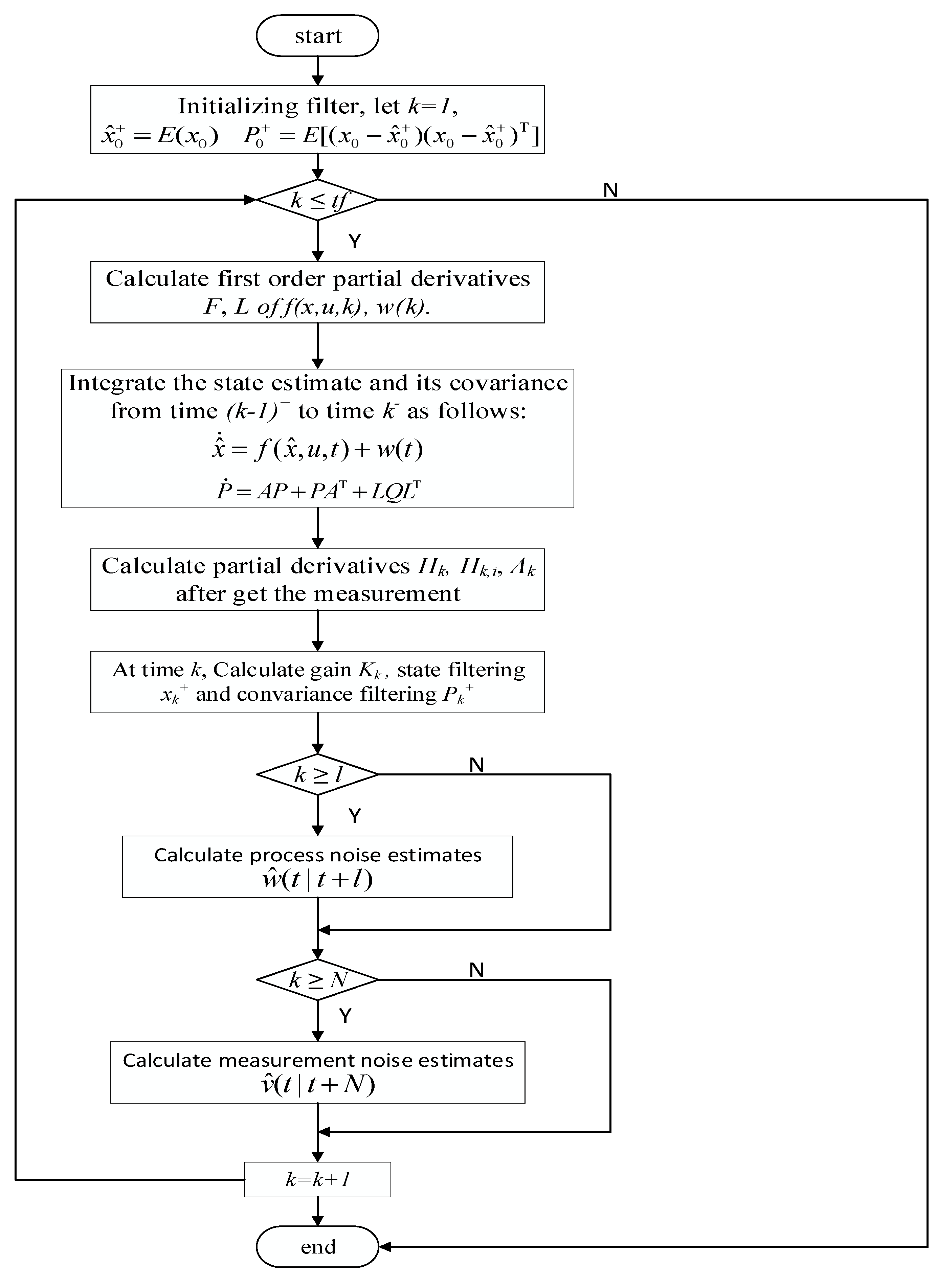
According to the theoretical derivation of Theorem 1 and Theorem 2, we can use a flowchart to represent the white noise estimation algorithm in the following Figure 1, where $k, l, N, and tf$ represent time, smoothing step of process noise, smoothing step of measurement noise, and end time, respectively.

Remark 2. 

The algorithm flow inFigure 1can be described as follows:

Step 1:Set${\widehat{x}}_0^{+}=x_0$,$P_0^{+}=P_0$,$k=1$,$l=l_0$,$N=N_0$and$tf=t{f}_0$.

Step 2:If$k\le tf$, go to Step 3; If$k>tf$, exit.

Step 3:Calculate$F, L$by Taylor expansion$f(x,u,k), w(k)$.

Step 4:Calculate$H_k, H_{k,i}, {\Lambda }_k$by Taylor expansion$h_k(x_k)$and (19).

Step 5:Integrate (5) and (6) from time${(k-1)}^{+}$to time$k^{-}$, obtain the${\widehat{x}}_k^{-}$and$P_k^{-}$.

Step 6:Calculate$K_k$by (17), then compute ${\widehat{x}}_k^{+}$,$P_k^{+}$using (16), (18).

Step 7:If$k>l$, calculate$\widehat{w}(t|t+l)$by (21).

Step 8:If$k>N$, calculate$\widehat{v}(k|k+N)$by (28).

Step 9:Set$k=k+1$, then go to Step 2.

4. Numerical Simulation

In this section, the first-order EKF and second-order EKF white noise estimators are compared by a numerical simulation; the advantages of the proposed algorithm is verified. Suppose the nonlinear continuous-discrete system (1) is as follows:

$$\{\begin{array}{c}\dot{x}=\cos (x(t))+w(t), \\ y_k=x_k^3+v_k, \end{array}$$

where the process noise vector $w(t)$ and measurement noise $v_k$ are uncorrelated zero-mean Gaussian white noises with variances $Q=0.0019$, and $R=0.0088$.

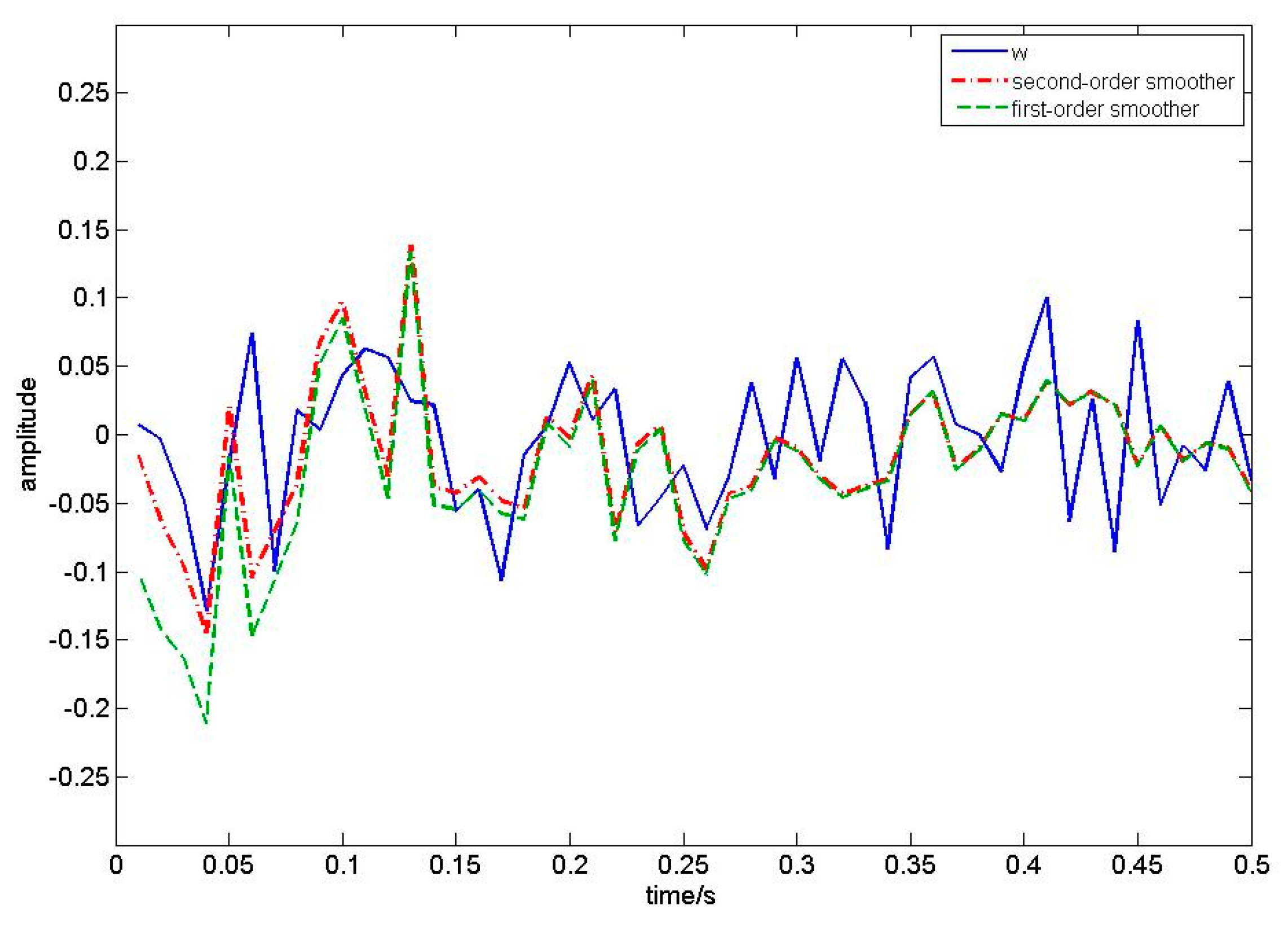
In this numerical simulation, we compare our algorithm with first-order EKF white noise estimators by setting that $x(0)=0.92$, $P(0)=0.08$ and the sampling period is 0.01s. We take 50 sampling periods to draw Figure 2, Figure 3, Figure 4 and Figure 5. According to Theorem 1, the filtering algorithm cannot achieve the process noise estimate. Therefore, in Figure 2, we use one-step smoothing algorithm to estimate the process noise. 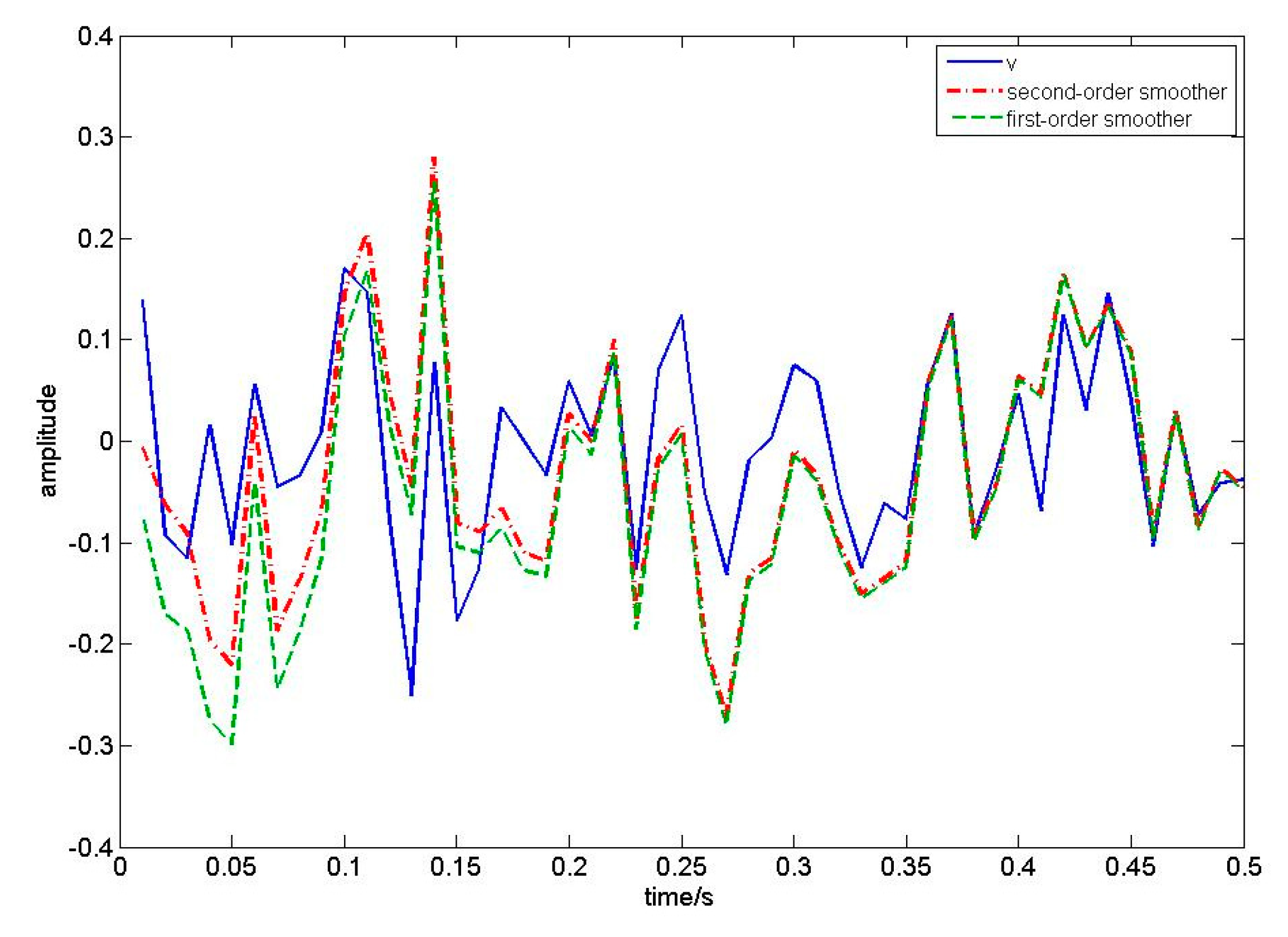Figure 2 shows the true value of process white noise $w(t)$and its one-step smoothing of two methods. 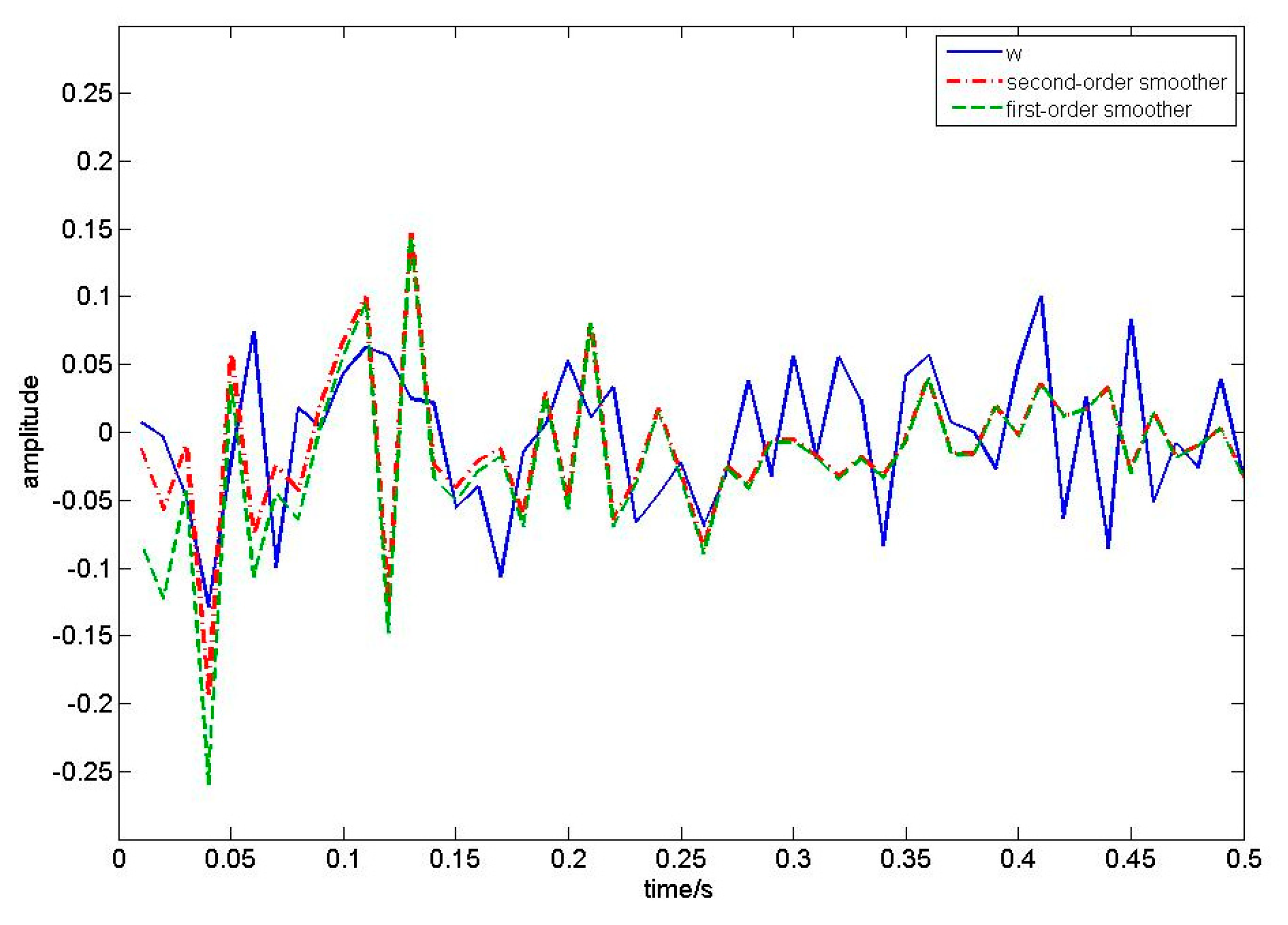Figure 3 shows the true value of process white noise $w(t)$ and its three-step smoothing of two methods. 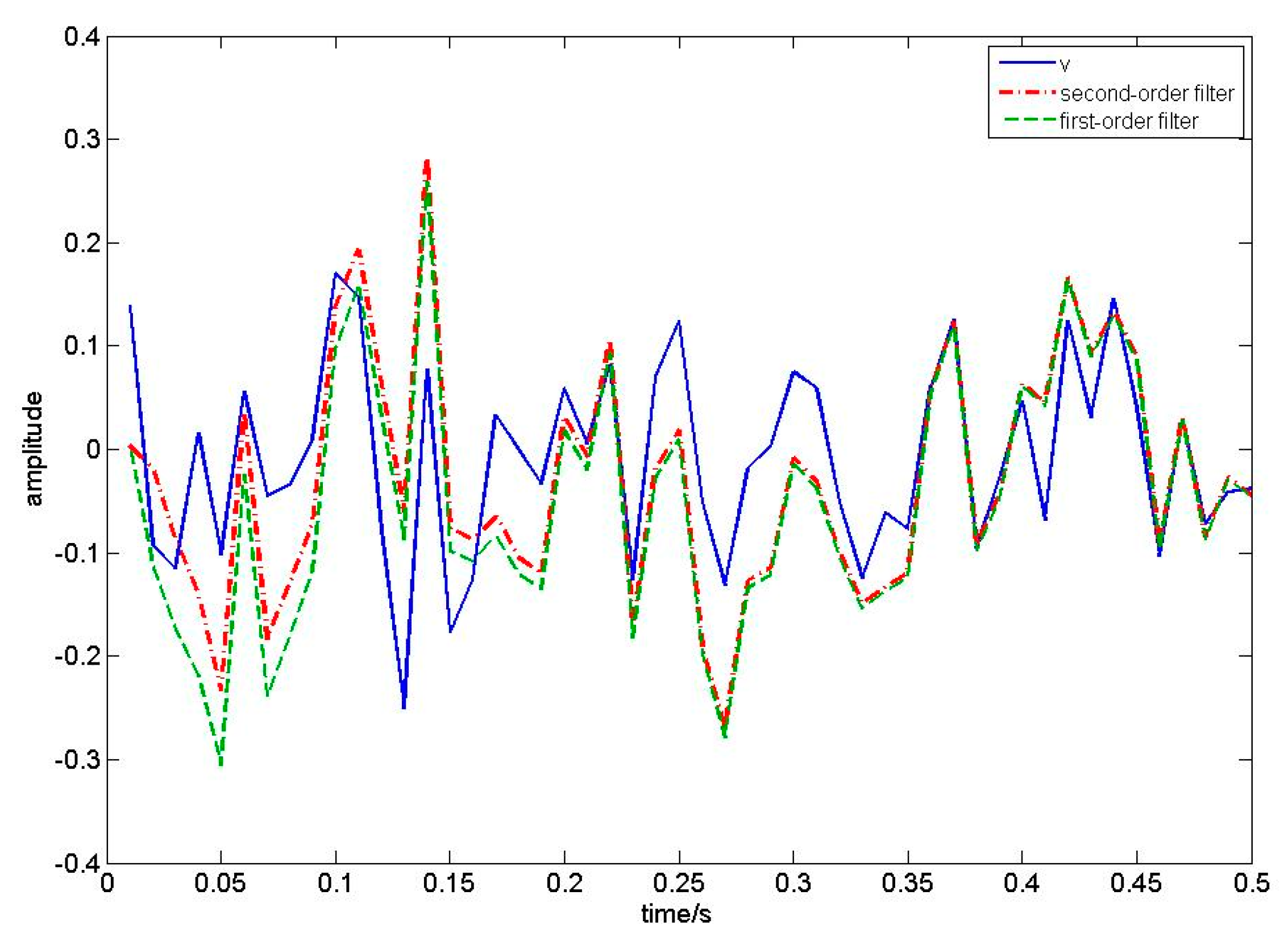Figure 4 shows the true value of measurement white noise $v_k$ and its filtering of two methods. Figure 5 shows the true value of measurement white noise $v_k$ and its three-step smoothing of two methods. From Figure 2 to Figure 5, it is shown that the white noise estimators based on the first-order EKF fluctuates greatly, while the estimator based on second-order EKF have higher estimation accuracy. In other words, the second-order EKF white noise estimators are better than the first-order EKF white noise estimators. Moreover, it can be seen that the process noise estimation is affected by the discrete observation equation, and loses some information. Therefore, the estimation effect is not as good as the measurement noise estimation. The measurement noise estimation will gradually approach the real curve with the update of time. Moreover, we take 50 sampling periods to calculate the error loss value of two different methods. Taking the mean square error (MSE) as the evaluation index, the loss value is shown in

Table 1. MSE of noise estimation.

MSE of Noise Estimated	First-Order EKF	Second-Order EKF
One-step smoothing of process noise	0.01011	0.00733
Three-step smoothing of process noise	0.01079	0.00884
Measurement noise filtering	0.01932	0.01540
Three-step smoothing of measurement noise	0.02239	0.01642

.

5. Discussion and Conclusions

For the nonlinear hybrid systems with continuous-time dynamic and discrete-time measurements, white noise estimators for process and measurement noises were designed in this paper. Firstly, the nonlinear second-order EKF was derived by using the projection formula after the second-order Taylor expansion approximation and the variance approximation. Moreover, the continuous process noise estimation was processed in segments, and the white noise estimation of the nonlinear hybrid system was performed by combining the innovation of the previous observation point with the second-order EKF theory. The observed white noise estimator was calculated by a difference equation solution of the Riccati equation. Finally, an example was presented to verify the effectiveness of the proposed algorithm.

This paper enriches the second-order EKF theory; the optimal white noise estimation theory is extended to the nonlinear hybrid systems. In the future, we will investigate the color noise estimation of nonlinear hybrid systems.