Convergence Analysis of a Modified Weierstrass Method for the Simultaneous Determination of Polynomial Zeros

Abstract

In 2016, Nedzhibov constructed a modification of the Weierstrass method for simultaneous computation of polynomial zeros. In this work, we obtain local and semilocal convergence theorems that improve and complement the previous results about this method. The semilocal result is of significant practical importance because of its computationally verifiable initial condition and error estimate. Numerical experiments to show the applicability of our semilocal theorem are also presented. We finish this study with a theoretical and numerical comparison between the modified Weierstrass method and the classical Weierstrass method.

1. Introduction

Throughout the present study, $(\mathbb{K},|·|)$ denotes an arbitrary normed field and $\mathbb{K}\left[z\right]$ represents the ring of polynomials over $\mathbb{K}$. The vector space ${\mathbb{K}}^n$ is equipped with p-norm ${\parallel ·\parallel }_p$ for some $1\le p\le \infty$ and with the vector norm $\parallel ·\parallel$ which are defined by

$${\parallel x\parallel }_p={\left(\sum _{i=1}^n{|x_i|}^p\right)}^{1/p}\mathrm{and}\parallel x\parallel =(|x_1|,\dots ,|x_n|).$$

Let $f\left(z\right)=a_0{z}^n+a_1{z}^{n-1}+\cdots +a_n$ be a polynomial in $\mathbb{K}\left[z\right]$ of degree $n\ge 2$. A vector $\xi \in {\mathbb{K}}^n$ is said to be a root-vector of f if

$$f\left(z\right)=a_0\prod _{i=1}^n(z-{\xi }_i)\mathrm{for}\mathrm{all}z\in \mathbb{K}.$$

In 1891, Weierstrass [1] established an iterative method for finding the root-vector of f. The famous Weierstrass method is defined in ${\mathbb{K}}^n$ by the iteration:

$$x^{(k+1)}=x^{\left(k\right)}-W_f\left(x^{\left(k\right)}\right),k=0,1,2,\dots ,$$

(1)

where the Weierstrass correction $W_f:\mathcal{D}\subset {\mathbb{K}}^n\to {\mathbb{K}}^n$ is defined as follows

$$W_f\left(x\right)=(W_1\left(x\right),\dots ,W_n\left(x\right))\mathrm{with}{W}_i\left(x\right)=\frac{f\left(x_i\right)}{a_0{\prod }_{j\ne i}(x_i-x_j)}(i=1,\dots ,n).$$

(2)

Apparently, the domain of $W_f$ is the set of the vectors in ${\mathbb{K}}^n$ with pairwise distinct components, that is, the set

$$\mathcal{D}=\left\{x\in {\mathbb{K}}^n:x_i\ne x_j\mathrm{whenever}i\ne j\right\}.$$

(3)

Since 1960, the Weierstrass method (1) has been rediscovered and studied by numerous authors and has became a powerful tool for constructing of new iterative methods for simultaneous finding of polynomial zeros (see, e.g., the monographs of Sendov, Andreev and Kyurkchiev [2], Kyurkchiev [3], Petković [4] and references therein). In 1962, Dochev [5] was the first who proved a theorem for local convergence of the Weierstrass method (1). For a detailed convergence analysis and historical survey about the Weierstrass method (1), we refer the reader to the papers [6,7,8,9,10].

Recently, Nedzhibov [11] established the following modification of the Weierstrass method:

$$x^{(k+1)}=T\left(x^{\left(k\right)}\right),k=0,1,2,\dots ,$$

(4)

where the iteration function $T:D\subset {\mathbb{K}}^n\to {\mathbb{K}}^n$ is defined by

$${\displaystyle T\left(x\right)=(T_1\left(x\right),\dots ,T_n\left(x\right))\mathrm{with}{T}_i\left(x\right)=\frac{x_i^2}{x_i+W_i\left(x\right)}(i\in I_n),}$$

(5)

where $W_i$ is defined by (2). This study deals with the convergence of the method (4) which will be called modified Weierstrass method. Note that the domain of the iteration function T is the set

$$D=\left\{x\in \mathcal{D}:x_i+W_i\left(x\right)\ne 0\mathrm{for}\mathrm{all}i\in I_n\right\}.$$

(6)

Here and throughout the whole paper, $I_n$ denotes the set of indices $1,\dots ,n$, i.e., $I_n=\{1,\dots ,n\}$.

In what follows, for a given p ($1\le p\le \infty$), we always define a number q by

$$1\le q\le \infty \mathrm{with}1/p+1/q=1$$

and for a given n, we use the following denotations:

$$a={(n-1)}^{1/q},b=2^{1/q}.$$

(7)

Note that $1\le a\le n-1$ and $1\le b\le 2$.

A local convergence analysis of the modified Weierstrass method (4) was presented in the papers [11,12,13,14,15,16]. More detaily, in [12] Nedzhibov proved the following convergence result:

Theorem 1

([12] (Theorem 3.6)). Let $f\in \mathbb{C}\left[z\right]$ be a monic polynomial of degree $n\ge 2$ possessing only simple roots and such that $f\left(0\right)\ne 0$. Let also $\xi \in {\mathbb{C}}^n$ be a root-vector of f and $1\le p\le \infty$. Suppose $x^{\left(0\right)}\in {\mathbb{C}}^n$ is an initial approximation satisfying

$$\tilde{E}\left(x^{\left(0\right)}\right)=\frac{\parallel x^{\left(0\right)}{-\xi \parallel }_p}{\tilde{\Delta }\left(\xi \right)}<\mu =\frac{\sqrt[n-1]{\theta }-1}{b(\sqrt[n-1]{\theta }-1)+a/(n-1)},$$

(8)

where

$$\tilde{\Delta }\left(\xi \right)=min\{\gamma \left(\xi \right),\delta \left(\xi \right)\}with\gamma \left(\xi \right)=\underset{i\in I_n}{min}|{\xi }_i|and\delta \left(\xi \right)=\underset{i\ne j}{min}|{\xi }_i-{\xi }_j|,$$

(9)

the numbers a, b are defined by (7) and the number θ is defined by

$$\theta =\frac{3b-2+\sqrt{b^2-4b+20}}{2(b+1)}.$$

(10)

Then the following statements hold true:

(i)

The modified Weierstrass iteration (4) is well defined and converges quadratically to the root-vector ξ of f.

(ii)

For all $k\ge 0$ the following estimates hold

$$\parallel x^{(k+1)}{-\xi \parallel }_p\le {\tilde{\lambda }}^{2^k}\parallel x^{\left(k\right)}{-\xi \parallel }_{p}and\parallel x^{\left(k\right)}{-\xi \parallel }_p\le {\tilde{\lambda }}^{2^k-1}{\parallel x^{\left(0\right)}-\xi \parallel }_p,$$

(11)

where $\tilde{\lambda }=\tilde{E}\left(x^{\left(0\right)}\right)/\mu$.

In [13] the following theorem that enlarges the convergence domain and improves the error estimates of Theorem 1 in the case $p=\infty$ was introduced:

Theorem 2.

Let $f\in \mathbb{C}\left[z\right]$ be a monic polynomial of degree $n\ge 2$ possessing only simple roots and such that $f\left(0\right)\ne 0$. Let $\xi \in {\mathbb{C}}^n$ be a root-vector of f and $x^{\left(0\right)}\in {\mathbb{C}}^n$ be an initial approximation satisfying

$$\tilde{E}\left(x^{\left(0\right)}\right)=\frac{\parallel x^{\left(0\right)}{-\xi \parallel }_{\infty }}{\tilde{\Delta }\left(\xi \right)}<\nu =\frac{\sqrt[n+1]{2}-1}{2\sqrt[n+1]{2}-1}$$

(12)

where $\tilde{\Delta }$ is defined by (9). Then the modified Weierstrass iteration (4) is well defined and converges quadratically to the root-vector ξ of f with error estimates

$$\parallel x^{(k+1)}{-\xi \parallel }_{\infty }\le {\tilde{\lambda }}^{2^k}\parallel x^{\left(k\right)}{-\xi \parallel }_{\infty }and\parallel x^{\left(k\right)}{-\xi \parallel }_{\infty }\le {\tilde{\lambda }}^{2^k-1}{\parallel x^{\left(0\right)}-\xi \parallel }_{\infty },$$

(13)

where $\tilde{\lambda }=\tilde{E}\left(x^{\left(0\right)}\right)/\nu$.

Remark 1.

Actually, Theorem 2 was exposed in p-norm settings but the proof given in [13] is not correct since it is based on an incorrect inequality. Namely, the second inequality of ([13] Equation (20)) is not true for $p=2$ and $n\ge 5$, $p=3$ and $n\ge 5$, $p=4$ and $n\ge 4$ etc.

Here is the version of Theorem 2 stated in [13].

Theorem 3

([13] (Theorem 2.6)). Let $f\in \mathbb{C}\left[z\right]$ be a monic polynomial of degree $n\ge 2$ possessing only simple roots and such that $f\left(0\right)\ne 0$. Let also $\xi \in {\mathbb{C}}^n$ be a root-vector of f and $1\le p\le \infty$. Suppose $x^{\left(0\right)}\in {\mathbb{C}}^n$ is an initial approximation satisfying

$$\tilde{E}\left(x^{\left(0\right)}\right)=\frac{\parallel x^{\left(0\right)}{-\xi \parallel }_p}{\tilde{\Delta }\left(\xi \right)}<\omega =\frac{\sqrt[n+1]{b}-1}{b(\sqrt[n+1]{b}-1)+a/(n-1)}$$

(14)

where $\tilde{\Delta }$ is defined by (9) and the quantities $a,b$ are defined by (7). Then the modified Weierstrass iteration (4) is well defined and converges quadratically to the root-vector ξ of f with error estimates (11), where $\tilde{\lambda }=\tilde{E}\left(x^{\left(0\right)}\right)/\omega$.

Under the assumptions of Theorem 2 an assessment of the asymptotic error constant of the modified Weierstrass iteration (4) was provided in the following convergence theorem:

Theorem 4

([16] (Theorem 1)). Let the assumptions of Theorem 2 are fulfilled. Then the following estimate of the asymptotic error constant holds:

$$\underset{k\to \infty }{lim\; sup}\frac{\parallel x^{(k+1)}{-\xi \parallel }_{\infty }}{\parallel x^{\left(k\right)}{-\xi \parallel }_{\infty }^2}\le \frac{n}{\tilde{\Delta }\left(\xi \right)}.$$

(15)

Very recently, based on the methods of [17] and Theorem 2 the following convergence theorem has been obtained in [14].

Theorem 5

([14] (Theorem 4)). Let $f\in \mathbb{C}\left[z\right]$ be a monic polynomial of degree $n\ge 2$. Suppose there exists a vector $x^{\left(0\right)}\in {\mathbb{C}}^n$ with distinct nonzero components such that

$$\frac{\parallel W_f\left(x^{\left(0\right)}\right){\parallel }_{\infty }}{\tilde{\Delta }\left(x^{\left(0\right)}\right)}\le \tilde{R}\left(n\right)=\frac{\tilde{R}(1-\tilde{R})}{1+(n-2)\tilde{R}},$$

(16)

where $\tilde{\Delta }$ is defined by (9) and $\tilde{R}=(\sqrt[n+1]{2}-1)/(4\sqrt[n+1]{2}-3)$. Then f has only simple zeros and the iteration (4) is well defined and converges quadratically to the root-vector ξ of f with error estimates (13).

It is important to note that Theorem 1 and Theorem 2 are independent. Theorem 5 as well as the results of [11] and [14] are direct consequences of Theorem 2. On the other hand, in the case $n\ge 3$, Theorem 4 generalizes and improves Theorem 1 of [15]. In other words, the above presented theorems (Theorems 1–5) cover all existing results about the modified Weierstrass method (4) except Theorem 1 of [15] in the case $n=2$.

In this paper, we obtain a local convergence theorem (Theorem 7) that improves and complements all above mentioned theorems (Theorems 1–5) including Theorem 1 of [15] in the case $n=2$. Furthermore, in Section 4 we prove a semilocal convergence theorem (Theorem 9) that improves and complements Theorem 5. In Section 5, we provide some numerical experiments to show the applicability of our semilocal convergence result. Finally, in Section 6 we provide theoretical end numerical comparisons that show the superiority of the classical Weierstrass method (1) over the modified Weierstrass method (4) in all considered aspects.

2. Preliminaries

Recently, Proinov [6,17,18,19,20] has developed a general convergence theory of the Picard type methods. The main role in the theory is played by a real-valued function called function of initial conditions of an iteration function T (Definition 3). Some implementations of this theory by using different functions of initial conditions can be found in [7,8,9,21,22,23,24,25,26,27,28,29].

The main aim of this section is to recall some definitions and theorems of Proinov [6,19] which are crucial for the proof of our results in this paper. First of all, we equip ${\mathbb{R}}^n$ with a coordinate-wise (partial) ordering $⪯$ defined by

$$x⪯y\mathrm{if}\mathrm{and}\mathrm{only}\mathrm{if}{x}_i\le y_i\mathrm{for}\mathrm{each}i\in I_n.$$

Furthermore, with J we denote an interval on ${\mathbb{R}}_{+}$ containing 0 and we assume by definition that $0^0=1$. We denote by $S_k\left(r\right)$ the sum of the first k terms of the sequence $1,r,r^2,\cdots$, i.e., for all $k\in \mathbb{N}$, we have

$$S_k\left(r\right)=1+r+\cdots +r^{k-1}.$$

(17)

In the case $k=0$, we set $S_0\left(r\right)=0$.

Definition 1

([19] (Definition 2.1)). A function $\phi :J\subset \mathbb{R}\to {\mathbb{R}}_{+}$ is called quasi-homogeneous of degree $r\ge 0$ if it is such that $\phi \left(\lambda t\right)\le {\lambda }^r\phi \left(t\right)$ for all $\lambda \in [0,1)$ and $t\in J$.

Recall some useful properties of the quasi-homogeneous functions [19].

• A function $\varphi$ is quasi-homogeneous of degree $r=0$ on an interval J if and only if $\varphi$ is nondecreasing on J;
• If $\varphi$ and $\phi$ are quasi-homogeneous of degree $r\ge 0$ on J, then $\varphi +\phi$ is also quasi-homogeneous of degree r on J;
• If $\varphi$ and $\phi$ are quasi-homogeneous of degree $p\ge 0$ and $q\ge 0$ on J, then $\varphi \phi$ is quasi-homogeneous of degree $p+q$ on J.

Proposition 1

([6] (Example 2.2)). Let $n\in \mathbb{N}$ and $\phi :J\to {\mathbb{R}}_{+}$ is a quasi-homogeneous function of degree $r>0$ on some interval J, then the following function:

$$\mathsf{\Phi }\left(t\right)={(1+\phi \left(t\right))}^n-1$$

is quasi-homogeneous of the same degree r on J.

Definition 2

([19] (Definition 2.4)). A function $\phi :J\to {\mathbb{R}}_{+}$ is called a gauge function of order $r\ge 1$ on J if it fulfills the following conditions:

(i)

φ is a quasi-homogeneous function of degree r on J;

(ii)

$\phi \left(t\right)\le t$ for all $t\in J$.

A gauge function φ of order r on J is called a strict gauge function if the last inequality holds strictly on $t\in J\setminus \left\{0\right\}$.

The following result gives a simple sufficient condition for gauge functions of order r.

Proposition 2

([19]). If $\phi :J\to {\mathbb{R}}_{+}$ is a quasi-homogeneous function of degree $r\ge 1$ on some interval J and $R>0$ is a fixed point of φ in J, then φ is a gauge function of order r on the interval $[0,R]$. Besides, if $r>1$, then φ is a strict gauge function of order r on $[0,R)$.

Definition 3

([19] (Definition 3.1)). Let X be an arbitrary set and $T:D\subset X\to X$. A function $E:D\to {\mathbb{R}}_{+}$ is called a function of initial conditions of T (with a gauge function φ on an interval J) if there is a function $\phi :J\to J$ such that

$$E\left(Tx\right)\le \phi \left(E\right(x\left)\right)forallx\in DwithTx\in DandE\left(x\right)\in J.$$

(18)

Definition 4

([19] (Definition 3.2)). Let X be an arbitrary set and $T:D\subset X\to X$. Suppose $E:D\to {\mathbb{R}}_{+}$ is a function of initial conditions of T (with gauge function on an interval J). Then a point $x\in D$ is called an initial point of T if $E\left(x\right)\in J$ and all of the iterates $T^n\left(x\right)$ $(n=0,1,\dots )$ are well defined and belong to D.

We shall use the following proposition as a detector for initial points.

Proposition 3

([19] (Proposition 4.1)). Let X be an arbitrary set, $T:D\subset X\to X$ and $E:D\to {\mathbb{R}}_{+}$ be a function of initial conditions of T with a gauge function φ on J. Assume that

$$x\in DwithE\left(x\right)\in JimpliesTx\in D.$$

Then every point $x^{\left(0\right)}\in D$ such that $E\left(x^{\left(0\right)}\right)\in J$ is an initial point of T.

Definition 5

([6] (Definition 3.1)). Let $T:D\subset X\to X$ be a map in a cone normed space $(X,\parallel ·\parallel )$ over a solid vector space $(Y,⪯)$ and $E:D\to {\mathbb{R}}_{+}$ be a function of initial conditions of T with a gauge function on an interval J. Then T is called an iterated contraction with respect to E at a point $\xi \in D$ (with control function ϕ) if $E\left(\xi \right)\in J$ and

$$\parallel Tx-\xi \parallel ⪯\varphi \left(E\right(x\left)\right)\parallel x-\xi \parallel forallx\in DwithE\left(x\right)\in J,$$

where $\varphi :J\to [0,1)$ is a nondecreasing function.

To prove our main theorem, we shall use the following general local convergence result of Proinov [6].

Theorem 6

([6] (Corollary 3.4)). Let $T:D\subset X\to X$ be a map in a cone normed space $(X,\parallel ·\parallel )$ over a solid vector space $(Y,⪯)$ and $E:D\to {\mathbb{R}}_{+}$ be a function of initial conditions of T with a strict gauge function φ of order r on some interval J. If T is an iterated contraction with respect to E at a point ξ with control function ϕ such that $\phi \left(t\right)=t\varphi \left(t\right)$ for all $t\in J$, then for every initial point $x^{\left(0\right)}$ of T the Picard iteration (4) remains in the set $U=\left\{x\in D:E\left(x\right)\in J\right\}$ and converges to ξ with error estimates

$$\parallel x^{(k+1)}-\xi \parallel ⪯{\lambda }^{r^k}\parallel x^{\left(k\right)}-\xi \parallel and\parallel x^{\left(k\right)}-\xi \parallel ⪯{\lambda }^{S_k\left(r\right)}\parallel x^{\left(0\right)}-\xi \parallel$$

for all $k\ge 0$, where $\lambda =\varphi \left(E\left(x^{\left(0\right)}\right)\right)$.

3. Local Convergence Analysis

Let $f\in \mathbb{K}\left[z\right]$ be a polynomial of degree $n\ge 2$ with n simple roots in $\mathbb{K}$ and such that $f\left(0\right)\ne 0$ and let $\xi \in {\mathbb{K}}^n$ be a root-vector of f. Afterwards, we define the function $d:{\mathbb{K}}^n\to {\mathbb{R}}^n$ by

$$d\left(x\right)=(d_1\left(x\right),\dots ,d_n\left(x\right))\mathrm{with}{d}_i\left(x\right)=\underset{j\ne i}{min}|x_i-x_j|(i\in I_n)$$

(19)

and the function $\Delta :{\mathbb{K}}^n\to {\mathbb{R}}^n$ by

$$\Delta \left(x\right)=({\Delta }_1\left(x\right),\dots ,{\Delta }_n\left(x\right))\mathrm{with}{\Delta }_i\left(x\right)=min\{|x_i|,d_i\left(x\right)\}(i\in I_n).$$

(20)

Also, for two vectors $x\in {\mathbb{K}}^n$ and $y\in {\mathbb{R}}^n$ we use the denotation $x/y$ for the vector in ${\mathbb{R}}^n$ defined by

$$\frac{x}{y}=\left(\frac{|x_1|}{y_1},\cdots ,\frac{|x_n|}{y_n}\right)$$

provided that y has only nonzero components.

In the present section, we study the convergence of the modified Weierstrass method (4) regarding the function of initial conditions $E:{\mathbb{K}}^n\to {\mathbb{R}}_{+}$ defined by

$$E\left(x\right)={∥\frac{x-\xi }{\Delta \left(\xi \right)}∥}_p(1\le p\le \infty ).$$

(21)

Note that, according to (9) and (20) we have ${\displaystyle \tilde{\Delta }\left(\xi \right)=\underset{i\in I_n}{min}{\Delta }_i\left(\xi \right)}$ and therefore

$$E\left(x\right)={∥\frac{x-\xi }{\Delta \left(\xi \right)}∥}_p\le \frac{{\parallel x-\xi \parallel }_p}{\tilde{\Delta }\left(\xi \right)}=\tilde{E}\left(x\right).$$

(22)

We start this section with two technical lemmas that will be used in the proofs of the forthcoming results.

Lemma 1

([6] (Proposition 5.5)). Let $u\in {\mathbb{K}}^n$ and $1\le p\le \infty$. Then the following inequalities hold:

$$\left|\prod _{j=1}^n(1+u_j)\right|\le {\left(1+\frac{{\parallel u\parallel }_p}{n^{1/p}}\right)}^{n}and\left|\prod _{j=1}^n(1+u_j)-1\right|\le {\left(1+\frac{{\parallel u\parallel }_p}{n^{1/p}}\right)}^n-1.$$

Lemma 2

([6] (Lemma 6.1)). Let $x,\xi \in {\mathbb{K}}^n$, vector ξ be with distinct components and $1\le p\le \infty$. Then for $i\ne j$,

$$|x_i-x_j|\ge (1-bE\left(x\right)){\Delta }_j\left(\xi \right)and|x_i-{\xi }_j|\ge (1-E\left(x\right)){\Delta }_i\left(\xi \right),$$

where b is defined by (7) and $E:{\mathbb{K}}^n\to {\mathbb{R}}_{+}$ is defined by (21).

In what follows, for $n\in \mathbb{N}$, we define the functions $\psi :[0,1/b)\to [1,\infty )$ and $\varphi :[0,\tau )\to {\mathbb{R}}_{+}$ by

$$\psi \left(t\right)={\left(1+\frac{at}{(n-1)(1-bt)}\right)}^{n-1}\mathrm{and}\varphi \left(t\right)=\frac{\psi \left(t\right)-1+t}{1-t-t\psi \left(t\right)},$$

(23)

where a and b are defined by (7) and $\tau$ is the unique solution of the equation

$$1-t-t\psi \left(t\right)=0$$

(24)

in the interval $(0,1/b)$. The existence and uniqueness of $\tau$ follow from the fact that the left hand side of (24) is decreasing function that maps $[0,1/b)$ onto $[1,-\infty )$. It must also be noted that the function $\varphi$ is quasi-homogeneous of the first degree on the interval $[0,\tau )$, pursuant to Proposition 1 and the last two of the aforementioned properties.

The main aim of the next lemma is to show that the function E defined by (21) is a function of initial conditions of the modified Weierstrass iteration function T defined by (5) as well as that the function T is an iterated contraction at $\xi$ with respect to E.

Lemma 3.

Let $f\in \mathbb{K}\left[z\right]$ be a polynomial of degree $n\ge 2$ with n simple roots in $\mathbb{K}$ and such that $f\left(0\right)\ne 0$, $\xi \in {\mathbb{K}}^n$ be a root-vector of f and $1\le p\le \infty$. Let $x\in {\mathbb{K}}^n$ be such that

$$E\left(x\right)<\tau ,$$

(25)

where the functions E is defined by (21) and τ is the unique solution of the Equation (24) in the interval $(0,1/b)$, where b is defined by (7). Then the following statements hold:

(i)

$x\in D$, where D is defined by (6);

(ii)

$\parallel Tx-\xi \parallel ⪯\varphi \left(E\right(x\left)\right)\parallel x-\xi \parallel$, where ϕ is defined by (23);

(iii)

$E\left(Tx\right)\le \phi \left(E\right(x\left)\right)$, where the real function φ is defined by $\phi \left(t\right)=t\varphi \left(t\right)$.

Proof. 

(i) We note that the first inequality of Lemma 2 and $E\left(x\right)<\tau <1/b$ imply that $x\in \mathcal{D}$. Let $i\in I_n$ be fixed. According to (6), we have to prove that

$$x_i+W_i\left(x\right)\ne 0.$$

(26)

From the triangle inequality and $E\left(x\right)<\tau <1$, we get

$$|x_i|=|{\xi }_i+x_i-{\xi }_i|\ge |{\xi }_i|-|x_i-{\xi }_i|\ge {\Delta }_i\left(\xi \right)-|x_i-{\xi }_i|=\left(1-\frac{|x_i-{\xi }_i|}{{\Delta }_i\left(\xi \right)}\right){\Delta }_i\left(\xi \right)\ge (1-E\left(x\right)){\Delta }_i\left(\xi \right)>0.$$

(27)

From the definition of $W_i\left(x\right)$, we have

$$W_i\left(x\right)=\frac{{\prod }_{j=1}^n(x_i-{\xi }_j)}{{\prod }_{j\ne i}(x_i-x_j)}=(x_i-{\xi }_i)\prod _{j\ne i}\frac{x_i-{\xi }_j}{x_i-x_j}=(x_i-{\xi }_i)\prod _{j\ne i}\left(1+u_j\right),\mathrm{where}{u}_j=\frac{x_j-{\xi }_j}{x_i-x_j}.$$

(28)

Observe that from the first inequality of Lemma 2, we get

$$|u_j|=\left|\frac{x_j-{\xi }_j}{x_i-x_j}\right|\le \frac{|x_j-{\xi }_j|}{(1-bE\left(x\right)){\Delta }_j\left(\xi \right)}\mathrm{and}\mathrm{therefore}{\parallel u\parallel }_p\le \frac{E\left(x\right)}{1-bE\left(x\right)}.$$

(29)

So, from (28), using the first inequality of Lemma 1 with $u_j=(x_j-{\xi }_j)/(x_i-x_j)$ and the second inequality of (29), we get

$$|W_i\left(x\right)|\le |x_i-{\xi }_i|{\left(1+\frac{aE\left(x\right)}{(n-1)(1-bE(x\left)\right)}\right)}^{n-1}=|x_i-{\xi }_i|\psi \left(E\left(x\right)\right).$$

(30)

Now, from the triangle inequality, (27), (30) and $E\left(x\right)<\tau$, we obtain

$$\begin{array}{ccc}\hfill |x_i+W_i\left(x\right)|& \ge & |x_i|-|W_i\left(x\right)|\ge (1-E\left(x\right)){\Delta }_i\left(\xi \right)-|x_i-{\xi }_i|\psi \left(E\left(x\right)\right)\hfill \\ \hfill & \ge & (1-E\left(x\right)-E\left(x\right)\psi \left(E\left(x\right)\right)){\Delta }_i\left(\xi \right)>0\hfill \end{array}$$

which proves (26).

(ii) We ought to prove that

$$|T_i\left(x\right)-{\xi }_i|\le \varphi \left(E\left(x\right)\right)|x_i-{\xi }_i|$$

(31)

for each $i\in I_n$. If $x_i={\xi }_i$ for some i, then (31) becomes an equality. Suppose $x_i\ne {\xi }_i$. In this case, from (27) and (30), we get the following estimate:

$$\left|\frac{W_i\left(x\right)}{x_i}\right|\le \frac{|x_i-{\xi }_i|\psi \left(E\left(x\right)\right)}{{\Delta }_i\left(\xi \right)(1-E\left(x\right))}\le \frac{E\left(x\right)\psi \left(E\right(x\left)\right)}{1-E\left(x\right)}.$$

(32)

From this and (25), we obtain

$$\left|1+\frac{W_i\left(x\right)}{x_i}\right|\ge 1-\left|\frac{W_i\left(x\right)}{x_i}\right|\ge \frac{1-E\left(x\right)-E\left(x\right)\psi \left(E\right(x\left)\right)}{1-E\left(x\right)}>0.$$

(33)

So, from (5), we obtain

$${\displaystyle T_i\left(x\right)-{\xi }_i=\frac{x_i^2}{x_i+W_i\left(x\right)}-{\xi }_i=x_i-{\xi }_i-\frac{W_i\left(x\right)}{{\displaystyle 1+\frac{W_i\left(x\right)}{x_i}}}=\left(1-\frac{{\displaystyle \frac{W_i\left(x\right)}{x_i-{\xi }_i}}}{{\displaystyle 1+\frac{W_i\left(x\right)}{x_i}}}\right)(x_i-{\xi }_i)={\sigma }_i(x_i-{\xi }_i),}$$

(34)

where ${\sigma }_i$ is defined by

$${\sigma }_i=\left({\displaystyle 1-\frac{W_i\left(x\right)}{x_i-{\xi }_i}+\frac{W_i\left(x\right)}{x_i}}\right){\left({\displaystyle 1+\frac{W_i\left(x\right)}{x_i}}\right)}^{-1}.$$

(35)

Pursuant to (34), to complete the proof of (31) it remains to estimate $|{\sigma }_i|$ from above. In order to do this, we use the second inequality of Lemma 1 with $u_j=(x_j-{\xi }_j)/(x_i-x_j)$, (28) and (29), and thus we reach the following estimate:

$$\left|1-\frac{W_i\left(x\right)}{x_i-{\xi }_i}\right|=\left|\prod _{j\ne i}\frac{x_i-{\xi }_j}{x_i-x_j}-1\right|\le {\left(1+\frac{aE\left(x\right)}{(n-1)(1-bE(x\left)\right)}\right)}^{n-1}-1=\psi \left(E\left(x\right)\right)-1.$$

(36)

Hence, from (35), using the triangle inequality and the estimates (32), (33) and (36), we obtain

$$|{\sigma }_i|\le \frac{{\displaystyle \left|{\displaystyle 1-\frac{W_i\left(x\right)}{x_i-{\xi }_i}}\right|+\left|\frac{W_i\left(x\right)}{x_i}\right|}}{\left|{\displaystyle 1+\frac{W_i\left(x\right)}{x_i}}\right|}\le \frac{{\displaystyle \psi \left(E\left(x\right)\right)-1+\frac{E\left(x\right)\psi \left(E\right(x\left)\right)}{1-E\left(x\right)}}}{{\displaystyle \frac{1-E\left(x\right)-E\left(x\right)\psi \left(E\right(x\left)\right)}{1-E\left(x\right)}}}=\varphi \left(E\left(x\right)\right)$$

(37)

which together with (34) leads to (31) which proves (ii).

Finally, dividing both sides of (31) by ${\Delta }_i\left(\xi \right)$ and taking p-norm, we get the inequality (iii) which completes the proof of the lemma. ☐

For the proposes of the main result, we define the function $\Phi :[0,1/b)\to {\mathbb{R}}_{+}$ by

$$\mathsf{\Phi }\left(t\right)=\frac{1+t}{1-t}{\left(1+\frac{at}{(n-1)(1-bt)}\right)}^{n-1}=\frac{1+t}{1-t}\psi \left(t\right),$$

(38)

where a and b are defined by (7) and $\psi$ is defined by (23).

The following theorem is the first main convergence result of this paper.

Theorem 7.

Let $f\in \mathbb{K}\left[z\right]$ be a polynomial of degree $n\ge 2$ possessing n simple roots in $\mathbb{K}$ and such that $f\left(0\right)\ne 0$, $\xi \in {\mathbb{K}}^n$ be a root-vector of f and $1\le p\le \infty$. Suppose $x^{\left(0\right)}\in {\mathbb{K}}^n$ is an initial approximation satisfying

$$E\left(x^{\left(0\right)}\right)={∥\frac{x^{\left(0\right)}-\xi }{\Delta \left(\xi \right)}∥}_p<\frac{1}{2^{1/q}}and\mathsf{\Phi }\left(E\left(x^{\left(0\right)}\right)\right)<2,$$

(39)

where the real function Φ is defined by (38). Then the following statements hold:

(i)

The modified Weierstrass iteration (4) is well defined and converges quadratically to ξ.

(ii)

For all $k\ge 0$, we have the following error estimates

$$\parallel x^{(k+1)}-\xi \parallel ⪯{\lambda }^{2^k}\parallel x^{\left(k\right)}-\xi \parallel \mathrm{and}\parallel x^{\left(k\right)}-\xi \parallel ⪯{\lambda }^{2^k-1}\parallel x^{\left(0\right)}-\xi \parallel ,$$

(40)

where $\lambda =\varphi \left(E\left(x^{\left(0\right)}\right)\right)$ with ϕ defined by (23).

(iii)

If $x^{\left(k\right)}\ne \xi$ for sufficiently large k, then we have the following estimate of the asymptotic error constant:

$$\underset{k\to \infty }{lim\; sup}\frac{\parallel x^{(k+1)}{-\xi \parallel }_p}{\parallel x^{\left(k\right)}{-\xi \parallel }_p^2}\le \frac{{(n-1)}^{1/q}+1}{\tilde{\Delta }\left(\xi \right)},$$

(41)

where $\tilde{\Delta }$ is defined by (9).

Proof. 

We shall apply Theorem 6 to the iteration function $T:D\subset {\mathbb{K}}^n\to {\mathbb{K}}^n$ defined by (5), the function $E:{\mathbb{K}}^n\to {\mathbb{R}}_{+}$ defined by (21) and the function $\phi \left(t\right)=t\varphi \left(t\right)$, where $\varphi$ is defined by (23).

It is easy to verify that $t\in (0,1/2^{1/q})$ with $\mathsf{\Phi }\left(t\right)<2$ is equivalent to $t\in (0,\tau )$, where $\tau$ is the unique solution of the Equation (24) in the interval $(0,1/2^{1/q})$. So, (39) allows us to apply Lemma 3. Let R be the unique solution of $\varphi \left(t\right)=1$ in the interval $(0,\tau )$. The existence and uniqueness of R follow from the fact that $\varphi$ is a continuous and strictly increasing function that maps $[0,\tau )$ onto ${\mathbb{R}}_{+}$. Since $\varphi$ is quasi-homogeneous of the first degree on the interval $[0,\tau )$, then the function $\phi$ defined by $\phi \left(t\right)=t\varphi \left(t\right)$ is quasi-homogeneous of second degree on $[0,\tau )$. Also, we have $\phi \left(R\right)=R$, i.e., R is a fixed point of the function $\phi$ in the interval $(0,\tau )$. According to Proposition 2, this means that $\phi$ is a strict gauge function of order $r=2$ on $J=[0,R)$. Hence, by Lemma 3 (iii), we deduce that E is a function of initial conditions of T. Since $E\left(\xi \right)=0\in J$, then from Lemma 3 (ii) and Definition 5 it follows that T is an iterated contraction with respect to E at $\xi$ with control function $\varphi$ defined by (23).

Further, applying Lemma 3 (i) to $x^{\left(0\right)}$, we get $x^{\left(0\right)}\in D$. Let $x\in D$ be such that $E\left(x\right)\in J$. We have $Tx\in {\mathbb{K}}^n$, inasmuch as $x\in D$. Since $\phi$ is a gauge function of order $r\ge 1$ on J, then by Lemma 3 (iii), we get $E\left(Tx\right)\le \phi \left(E\right(x\left)\right)\le E\left(x\right)$ which means that $E\left(Tx\right)\in J$. Thus we have both $Tx\in {\mathbb{K}}^n$ and $E\left(Tx\right)\in J$. So, applying Lemma 3 (i) to $Tx$, we conclude that $Tx\in D$. According to Proposition 3, $x^{\left(0\right)}$ is an initial point of T. Consequently, the conclusions (i) and (ii) of Theorem 7 follow from Theorem 6.

It remains to prove the estimate (41). Since the function $\varphi$ defined by (23) is quasi-homogeneous of the first degree on the interval $[0,\tau )$, then the function $\varphi \left(t\right)/t$ is nondecreasing on $(0,\tau )$ (see [19] (Lemma 2.2)). So, according to Lemma 3 (ii) and the inequality (22), we obtain

$$\parallel x^{(k+1)}{-\xi \parallel }_p\le \varphi \left(E\left(x^{\left(k\right)}\right)\right)\parallel x^{\left(k\right)}{-\xi \parallel }_p=\frac{\varphi \left(E\left(x^{\left(k\right)}\right)\right)}{E\left(x^{\left(k\right)}\right)}E\left(x^{\left(k\right)}\right)\parallel x^{\left(k\right)}{-\xi \parallel }_p\le \frac{\varphi \left(E\left(x^{\left(k\right)}\right)\right)}{E\left(x^{\left(k\right)}\right)\tilde{\Delta }\left(\xi \right)}{\parallel x^{\left(k\right)}-\xi \parallel }_p^2.$$

Dividing both sides of this inequality by $\parallel x^{\left(k\right)}{-\xi \parallel }_p^2$ and taking lim sup, we get

$$\underset{k\to \infty }{lim\; sup}\frac{\parallel x^{(k+1)}{-\xi \parallel }_p}{\parallel x^{\left(k\right)}{-\xi \parallel }_p^2}\le \frac{1}{\tilde{\Delta }\left(\xi \right)}\underset{k\to \infty }{lim}\frac{\varphi \left(E\left(x^{\left(k\right)}\right)\right)}{E\left(x^{\left(k\right)}\right)}.$$

(42)

Further, according to the definitions of $\varphi$ and $\psi$, we get the following limit:

$$\underset{t\to 0}{lim}\frac{\varphi \left(t\right)}{t}=\underset{t\to 0}{lim}\frac{\psi \left(t\right)-1+t}{t(1-t-t\psi (t\left)\right)}=1+\underset{t\to 0}{lim}\frac{\psi \left(t\right)-1}{t}={(n-1)}^{1/q}+1.$$

Hence, taking into account that $E\left(x^{\left(k\right)}\right)\to 0$ as $k\to \infty$, from (42), we obtain (41) which completes the proof of the theorem. ☐

The following corollary of Theorem 7 improves and complements Theorem 1.

Corollary 1.

Let $f\in \mathbb{K}\left[z\right]$ be a polynomial of degree $n\ge 2$ with n simple roots in $\mathbb{K}$ and such that $f\left(0\right)\ne 0$. Let $\xi \in {\mathbb{K}}^n$ be a root-vector of f and $1\le p\le \infty$. Suppose $x^{\left(0\right)}\in {\mathbb{K}}^n$ is an initial approximation satisfying

$$E\left(x^{\left(0\right)}\right)={∥\frac{x^{\left(0\right)}-\xi }{\Delta \left(\xi \right)}∥}_p<R=\frac{\sqrt[n-1]{h}-1}{b(\sqrt[n-1]{h}-1)+a/(n-1)},$$

(43)

where $a,b$ are defined by (7) and the number h is defined by

$$h=\frac{3b-a-1+\sqrt{{(3b-a-1)}^2+8(b+1)(a+1-b)}}{2(b+1)}.$$

(44)

Then the iterative sequence (4) is well defined and converges quadratically to ξ with error estimates (40) and (41).

Proof. 

We ought to prove that $x^{\left(0\right)}$ satisfies (39). The first inequality of (39) is satisfied because of the inequality $R<1/b$. Since the function $\mathsf{\Phi }$ defined by (38) is strictly increasing on the interval $[0,R]$, then to prove the second inequality of (39) it is sufficient to show that $\mathsf{\Phi }\left(R\right)\le 2$. First, we note that R is the unique solution of the equation

$$\psi \left(t\right)=h$$

in the interval $[0,1/b)$, where h is defined by (44). So, applying Bernoulli’s inequality, we get

$$h=\psi \left(R\right)={\left(1+\frac{aR}{(n-1)(1-bR)}\right)}^{n-1}\ge 1+\frac{aR}{1-bR}.$$

(45)

From this, we obtain the following inequality:

$$R\le \frac{h-1}{b(h-1)+a}.$$

(46)

On the other hand, h is the unique positive root of the equation

$$(b+1)t^2-(3b-a-1)t-2(a+1-b)=0.$$

Therefore, we have the following identity:

$$\frac{(b+1)h^2-(b-a+1)h}{(b-1)h+a+1-b}=2.$$

(47)

From this, the definition of the function $\mathsf{\Phi }$ and the inequality (46), we get

$$\mathsf{\Phi }\left(R\right)=\frac{1+R}{1-R}\psi \left(R\right)\le \frac{b(h-1)+a+h-1}{b(h-1)+a-h+1}h=\frac{(b+1)h^2-(b-a+1)h}{(b-1)h+a+1-b}=2$$

which completes the proof. ☐

Comparison between Theorem 7 and Theorem 1.

We shall prove that Corollary 1 improves Theorem 1 in the following two directions:

First, Corollary 1 gives a larger convergence domain, i.e., every vector $x^{\left(0\right)}$ that satisfies the initial condition (8) satisfies (43) but not vice versa. This claim follows from the inequalities (22) and $\mu \le R$. The last inequality is equivalent to $\theta \le h$ which in turn follows from the fact that $h=h(a,b)$ is strictly increasing for $a\in [1,\infty )$ and $h=\theta$ when $a=1$.

Second, Corollary 1 provides better error estimates. Indeed, according to (43) the error estimates (11) follow from (40) because of the inequality $\lambda \le \tilde{\lambda }$. To prove the last inequality, we define R as the unique solution of $\varphi \left(t\right)=1$ in the interval $(0,\tau )$, where the function $\varphi :[0,\tau )\to {\mathbb{R}}_{+}$ is defined by (23). Recall that such R exists (see the proof of Theorem 7). Since, the function ϕ is quasi-homogeneous of the first degree on the interval $[0,R]$, then according to the increasement of $\varphi \left(t\right)/t$ on $(0,R]$ (see [19]), the inequalities (22), (43) and $\mu \le R$, we get

$$\lambda =\varphi \left(E\left(x^{\left(0\right)}\right)\right)=E\left(x^{\left(0\right)}\right)\frac{\varphi \left(E\left(x^{\left(0\right)}\right)\right)}{E\left(x^{\left(0\right)}\right)}\le E\left(x^{\left(0\right)}\right)\frac{\varphi \left(R\right)}{R}=\frac{E\left(x^{\left(0\right)}\right)}{R}\le \frac{\tilde{E}\left(x^{\left(0\right)}\right)}{\mu }=\tilde{\lambda }.$$

Corollary 1 complements Theorem 1 with the estimate (41).

In the case $p=\infty$ from Theorem 7, we obtain the following result:

Corollary 2.

Let $f\in \mathbb{K}\left[z\right]$ be a polynomial of degree $n\ge 2$ with n simple roots in $\mathbb{K}$ such that $f\left(0\right)\ne 0$ and $\xi \in {\mathbb{K}}^n$ be a root-vector of f. Suppose $x^{\left(0\right)}\in {\mathbb{K}}^n$ is an initial approximation satisfying

$$E\left(x^{\left(0\right)}\right)={∥\frac{x^{\left(0\right)}-\xi }{\Delta \left(\xi \right)}∥}_{\infty }<\frac{1}{2}and\Phi \left(E\left(x^{\left(0\right)}\right)\right)<2,$$

(48)

where the real function Φ is defined by

$$\mathsf{\Phi }\left(t\right)=\frac{1+t}{1-t}{\left(1+\frac{t}{1-2t}\right)}^{n-1}.$$

(49)

Then the modified Weierstrass iteration (4) is well defined and converges quadratically to ξ with error estimates (40), where $\lambda =\varphi \left(E\left(x^{\left(0\right)}\right)\right)$ with ϕ defined by (23) but with $a=n-1$ and $b=2$. Also, for all $k\ge 0$, we have the estimate of the asymptotic error constant (15).

Comparison between Theorem 7 and Theorem 2 and 4.

First, we shall prove that Corollary 2 gives a larger convergence domain than Theorem 2. To do this, we have to show that the initial condition (12) implies (48), i.e., we have to show that $\nu <1/2$ and $\mathsf{\Phi }\left(\nu \right)<2$, where ν is defined by (12) and the function Φ is defined by (49). The first inequality is obvious and the second one is equivalent to the inequality

$$\frac{3\sqrt[n+1]{2}-2}{\sqrt[n+1]{8}}<1$$

which holds for all $n\ge 2$. Really, putting $x=\sqrt[n+1]{2}$ in the last inequality, we get the inequality

$${(x-1)}^2(x+2)>0$$

which obviously holds for all $x\in (1,\infty )$.

Second, according to (48) the error estimates (13) follow from (40) due to the inequality (see the anterior comparison)

$$\lambda =\varphi \left(E\left(x^{\left(0\right)}\right)\right)\le \tilde{E}\left(x^{\left(0\right)}\right)/\nu =\tilde{\lambda }.$$

Theorem 7 gives a better assessment of the asymptotic error constant (41) than Theorem 4 owing to the inequality ${(n-1)}^{1/q}+1\le n$ for all $n\ge 2$ and $1\le q\le \infty$.

In what follows, we give a computer-assisted proof that Theorem 7 improves and complements even Theorem 3.

Comparison between Theorem 7 and Theorem 3.

To prove that Theorem 7 gives a larger convergence domain, we ought to show that $\omega <1/2^{1/q}$ and $\mathsf{\Phi }\left(\omega \right)<2$, where the function Φ is defined by (38). The first inequality is obvious. We shall prove the second one graphically. It is easy to verify that it is equivalent to the inequality

$$\frac{(b+1)(\sqrt[n+1]{b}-1)+a/(n-1)}{(b-1)(\sqrt[n+1]{b}-1)+a/(n-1)}\sqrt[n+1]{b^{n-1}}<2,$$

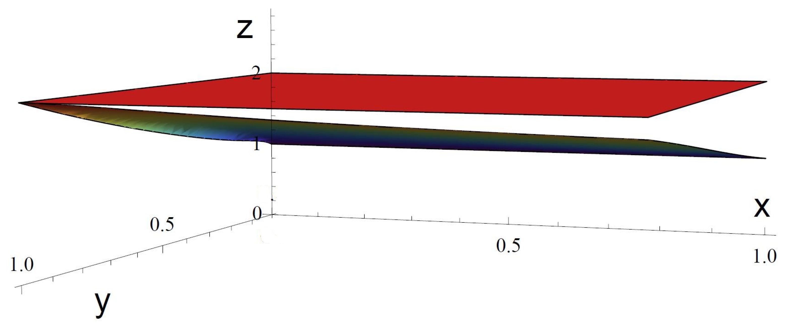
where a and b are defined by (7). Setting $x=1/(n-1)$ and $y=1/q$ in the last inequality, we get the inequality $G(x,y)\le 2$, where the function $G:(0,1]\times [0,1]\to \mathbb{R}$ is defined by

$$G(x,y)=\frac{x^y(2{}^y+1)(2{}^{xy/(2x+1)}-1)+x}{x^y(2{}^y-1)(2{}^{xy/(2x+1)}-1)+x}2{}^{y/(2x+1)}.$$

(50)

The graph of the function $z=G(x,y)$ is exhibited on Figure 1. One can see that the graph of G is beneath the plane $z=2$ for all $(x,y)\in (0,1]\times [0,1]$. Hence, we have $G(x,y)<2$ which implies $\mathsf{\Phi }\left(\nu \right)<2$ and therefore the initial condition (14) implies (39).

The error estimates of Theorem 3 follow immediately from (40) owing to the inequality (see the anterior comparison)

$$\lambda =\varphi \left(E\left(x^{\left(0\right)}\right)\right)\le \tilde{E}\left(x^{\left(0\right)}\right)/\omega =\tilde{\lambda }.$$

Theorem 7 complements Theorem 3 with the assessment (41).

4. Semilocal Convergence Analysis

Let $f\in \mathbb{K}\left[z\right]$ be a polynomial of degree $n\ge 2$. In the present section, we establish a new semilocal convergence result for the modified Weierstrass method (4) that generalizes and improves Theorem 5. We study the convergence of the iteration (4) regarding the function of initial conditions $E_f:\mathcal{D}\subset {\mathbb{K}}^n\to {\mathbb{R}}_{+}$ defined as follows

$$E_f\left(x\right)={∥\frac{W_f\left(x\right)}{\Delta \left(x\right)}∥}_p(1\le p\le \infty ),$$

(51)

where $\Delta :{\mathbb{K}}^n\to {\mathbb{R}}^n$ is defined by (20) and $W_f$ is Weierstrass correction defined by (2). Observe that the domain $\mathcal{D}$ of $E_f$ is the set

$$\mathcal{D}=\{x\in \mathcal{D}:x_i\ne 0,\mathrm{for}\mathrm{all}i\in I_n\}.$$

Recently, Proinov [17] showed that from any local convergence theorem about a simultaneous method one can obtains a semilocal convergence theorem about the same method. He classified the initial conditions into three types (see [17] (Definition 2.1)) and showed how initial conditions of the first and the second type (which are of rather theoretical importance) can be transformed into initial conditions of the third type that are of significant practical importance. Now, we note that all results of [17] remain true if one replaces the function d defined by (19) with the function $\Delta$ defined by (20) (see also [17] (Remark 2.2)). This means that we can apply the results of [17] to the functions E and $E_f$ defined by (21) and (51) as well. In what follows, we transform our Corollary 1 into a semilocal convergence theorem (Theorem 9) using the following version of Theorem 6.1 of Proinov [17]:

Theorem 8.

Let $f\in \mathbb{K}\left[z\right]$ be a polynomial of degree $n\ge 2$, and let there exists a vector $x\in {\mathbb{K}}^n$ with distinct components such that

$$E_f\left(x\right)={∥\frac{W_f\left(x\right)}{\Delta \left(x\right)}∥}_p\le \frac{R(1+(b-1\left)R\right)}{(1+bR)(1+(a+b-1\left)R\right)}$$

(52)

for some $1\le p\le \infty$ and $0<R\le 1/(1-b+\sqrt{a})$, where a and b are defined by (7) and $W_f$ is the Weierstrass correction defined by (2). Then f has only simple zeros and there exists a root-vector $\xi \in {\mathbb{K}}^n$ of f which satisfies

$${∥\frac{x-\xi }{\Delta \left(\xi \right)}∥}_p\le R.$$

(53)

For the purposes of our next result, we define a distance $\rho (x,y)$ between two vectors $x,y\in {\mathbb{K}}^n$ by (see, e.g., [10]):

$$\rho (x,y)=\underset{u\equiv y}{min}{\parallel x-u\parallel }_p,$$

where the binary relation $\equiv$ is defined on ${\mathbb{K}}^n$ as follows: $u\equiv y$ if there exists a permutation $(i_1,\dots ,i_n)$ of the indexes $(1,\dots ,n)$ such that $(u_1,\dots ,u_n)=(y_{i_1},\dots ,y_{i_n})$.

Now we are ready to state and prove the third main result of this paper. It is a theorem of significant practical importance since the initial condition and the error estimate are computationally verifiable.

Theorem 9.

Let $f\in \mathbb{K}\left[z\right]$ be a polynomial of degree $n\ge 2$, and let $x^{\left(0\right)}\in {\mathbb{K}}^n$ be an initial approximation with pairwise distinct nonzero components satisfying

$$E_f\left(x^{\left(0\right)}\right)={∥\frac{W_f\left(x^{\left(0\right)}\right)}{\Delta \left(x^{\left(0\right)}\right)}∥}_p<R(n,p)=\frac{R(1+(b-1\left)R\right)}{(1+bR)(1+(a+b-1\left)R\right)},$$

(54)

for some $1\le p\le \infty$, where $W_f$ is the Weierstrass correction defined by (2) and the number R is defined by (43). Then the following statements hold true:

(i)

The polynomial f possess only simple zeros in $\mathbb{K}$.

(ii)

The iteration (4) is well defined and converges quadratically to a root-vector ξ of f.

(iii)

For all $k\ge 0$ such that ${\mathcal{E}}_f\left(x^{\left(k\right)}\right)<1/{(1+\sqrt{a})}^2$, we have the following a posteriori error estimate

$$\rho (x^{\left(k\right)},\xi )\le \alpha \left({\mathcal{E}}_f\left(x^{\left(k\right)}\right)\right){\parallel W_f\left(x^{\left(k\right)}\right)\parallel }_p,$$

(55)

where the function ${\mathcal{E}}_f$ is defined by ${\mathcal{E}}_f\left(x\right)={\parallel W_f\left(x\right)/d\left(x\right)\parallel }_p$ and the real function α is defined by

$$\alpha \left(t\right)=2/\left(1-(a-1)t+\sqrt{{(1-(a-1)t)}^2-4t}\right).$$

(56)

Proof. 

Since $R\le 1/(1-b+\sqrt{a})$, then from (54) and Theorem 8 it follows that f possess only simple zeros and there exists a root-vector $\xi \in {\mathbb{K}}^n$ of f such that

$${∥\frac{x^{\left(0\right)}-\xi }{\Delta \left(\xi \right)}∥}_p<R.$$

From this and Corollary 1 it follows that the iteration (4) is well defined and converges quadratically to a root-vector $\xi$ of f. The estimate (55) follows from Theorem 5.1 of [17]. ☐

Remark 2.

In the case $p=\infty$, Theorem 9 gives a larger convergence domain than Theorem 5. Indeed, the initial condition (16) implies (54) due to the inequalities $\tilde{R}\left(n\right)<R(n,\infty )$ and

$${∥\frac{W_f\left(x\right)}{\Delta \left(x\right)}∥}_{\infty }\le \frac{\parallel W_f{\left(x\right)\parallel }_{\infty }}{\tilde{\Delta }\left(x\right)}.$$

Moreover, Theorem 9 provides a computationally verifiable error estimate unlike Theorem 5.

5. Applications

In this section, we show the applicability of our semilocal convergence result (Theorem 9). Our main aim is to show that Theorem 9 can be used for solving of two important practical problems: (i) numerical proof of the convergence of the modified Weierstrass method (4) and (ii) numerical proof of the accuracy of approximation at any iteration. For the sake of convenience, we consider the case $p=\infty$.

Suppose $f\in \mathbb{C}\left[z\right]$ is a polynomial of degree $n\ge 2$ and $x^{\left(0\right)}\in {\mathbb{C}}^n$ is an initial approximation. We apply the modified Weierstrass method (4) for computing all the zeros of f simultaneously. Applying Theorem 9 to $x^{\left(m\right)}$ instead of $x^{\left(0\right)}$, we get the following convergence criterion:

Convergence criterion.

If there exists an integer $m\ge 0$ for which

$$E_f\left(x^{\left(m\right)}\right)={∥\frac{W_f\left(x^{\left(m\right)}\right)}{\Delta \left(x^{\left(m\right)}\right)}∥}_{\infty }<{\mathcal{R}}_n=\frac{\mathcal{R}(1+\mathcal{R})}{(1+2\mathcal{R})(1+n\mathcal{R})},$$

(57)

where $\Delta :{\mathbb{C}}^n\to {\mathbb{R}}^n$ is defined by (20), $W_f$ is the Weierstrass correction defined by (2) and the number $\mathcal{R}$ is defined by

$$\mathcal{R}=\frac{\sqrt[n-1]{h}-1}{2\sqrt[n-1]{h}-1}withh=\frac{6-n+\sqrt{n^2+12n-12}}{6},$$

(58)

then f has only simple zeros in $\mathbb{C}$ and the iteration (4) is well-defined and is quadratically convergent to a root-vector ξ of f.

Next, applying Theorem 9 (iii) to $x^{\left(k\right)}$ instead of $x^{\left(0\right)}$, we get the following accuracy criterion:

Accuracy criterion.

If for a preset accuracy $\epsilon >0$ there exists an integer $k\ge 0$ for which

$${\mathcal{E}}_f\left(x^{\left(k\right)}\right)={∥\frac{W_f\left(x^{\left(k\right)}\right)}{d\left(x^{\left(k\right)}\right)}∥}_{\infty }<{\tau }_n=\frac{1}{{(1+\sqrt{n-1})}^2}and{\epsilon }_k<\epsilon ,$$

(59)

where the function $d:{\mathbb{C}}^n\to {\mathbb{R}}^n$ is defined by (19) and

$${\epsilon }_k=\alpha \left({\mathcal{E}}_f\left(x^{\left(k\right)}\right)\right){\parallel W_f\left(x^{\left(k\right)}\right)\parallel }_{\infty }$$

(60)

with α defined by (56) with $a=n-1$, then the root-vector ξ of f is calculated with accuracy ε. Besides, the accuracy ${\epsilon }_k$ is guaranteed at the kth iteration.

Henceforward, we consider the following polynomials ([5,9,23,30,31]):

$$\begin{array}{ccc}\hfill f_1\left(z\right)& =& z^3-8z^2-23z+30,\hfill \\ \hfill f_2\left(z\right)& =& z^3-(2+5i)z^2-(3-10i)z+15i,\hfill \\ \hfill f_3\left(z\right)& =& z^4-1,\hfill \\ \hfill f_4\left(z\right)& =& z^4-(1+i)z^3+(2+3i)z^2+(4+4i)z-24-12i,\hfill \\ \hfill f_5\left(z\right)& =& z^5-15z^4+22z^3+438z^2-1175z+1575,\hfill \\ \hfill f_6\left(z\right)& =& z^7+z^5-10z^4-z^3-z+10,\hfill \\ \hfill f_7\left(z\right)& =& z^8-1,\hfill \\ \hfill f_8\left(z\right)& =& z^9+3z^8-3z^7-9z^6+3z^5+9z^4+99z^3+297z^2-100z-300,\hfill \\ \hfill f_9\left(z\right)& =& z^{10}-1,\hfill \\ \hfill f_{10}\left(z\right)& =& z^{15}+z^{14}+1\hfill \end{array}$$

(61)

with Aberth’s initial approximation $x^{\left(0\right)}\in {\mathbb{C}}^n$ defined by ([32])

$$x_j^{\left(0\right)}=-\frac{a_1}{n}+r{e}^{i{\theta }_j},{\theta }_j=\frac{\pi }{n}\left(2j-\frac{3}{2}\right),j=1,\dots ,n,$$

(62)

where $r=34.61$ is randomly chosen from the interval (2, 1576) while $a_1$ and n are the second coefficient and the degree of the corresponding polynomial. For any of the polynomials, we calculate the smallest integer $m\ge 0$ that fulfills the convergence criterion (57) and the smallest integer $k\ge 0$ that satisfies the accuracy criterion (59) with accuracy $\epsilon ={10}^{-15}$. The values of m, $E_f\left(x^{\left(m\right)}\right)$ and ${\mathcal{R}}_n$ are given in

Table 1. Numerical data abut the convergence criterion (57).

Polynomial	$m$	$E_f\left(x^{\left(m\right)}\right)$	${\mathcal{R}}_{\mathbf{n}}$
$f_1$	12	$0.072910$	$0.090245$
$f_2$	The method is not well-defined
$f_3$	18	$0.038420$	$0.072327$
$f_4$	14	$0.070493$	$0.072327$
$f_5$	22	$0.023086$	$0.060653$
$f_6$	30	$0.029853$	$0.046138$
$f_7$	32	$0.035323$	$0.041277$
$f_8$	34	$0.005537$	$0.037367$
$f_9$	40	$0.004927$	$0.034149$
$f_{10}$	58	$0.002062$	$0.023943$

with at least six decimal digits. For instance, one can see from the table that for $f_1$ the convergence criterion (57) is fulfilled at twelfth step. On the other hand, for $f_2$, at the fourteenth step the MWM is not well defined. Besides, $E_f\left(x^{\left(14\right)}\right)=4.818\times {10}^{92}$.

In

Table 2. Numerical data about the accuracy criterion (59).

Polynomial	Method	$k$	$E_f\left(x^{\left(k\right)}\right)$	${\tau }_n$	${\epsilon }_k$
$f_1$	$MWM$	17	$2.330\times {10}^{-16}$	$0.171573$	$9.320\times {10}^{-16}$
	$WM$	10	$1.489\times {10}^{-16}$	$0.171573$	$5.958\times {10}^{-16}$	${\epsilon }_{17}=5.645\times {10}^{-2026}$
$f_2$	$MWM$	Diverges
	$WM$	29	$3.262\times {10}^{-31}$	$0.171573$	$1.304\times {10}^{-30}$
$f_3$	$MWM$	22	$6.444\times {10}^{-15}$	$0.133975$	$9.113\times {10}^{-16}$
	$WM$	18	$5.472\times {10}^{-23}$	$0.133975$	$7.738\times {10}^{-23}$	${\epsilon }_{22}=7.247\times {10}^{-352}$
$f_4$	$MWM$	18	$1.063\times {10}^{-17}$	$0.133975$	$2.378\times {10}^{-17}$
	$WM$	15	$5.549\times {10}^{-21}$	$0.133975$	$4.970\times {10}^{-26}$	${\epsilon }_{18}=1.355\times {10}^{-205}$
$f_5$	$MWM$	26	$2.957\times {10}^{-24}$	$0.111111$	$8.207\times {10}^{-24}$
	$WM$	15	$1.359\times {10}^{-20}$	$0.111111$	$3.772\times {10}^{-20}$	${\epsilon }_{26}=4.710\times {10}^{-40687}$
$f_6$	$MWM$	34	$2.410\times {10}^{-27}$	$0.084040$	$3.408\times {10}^{-27}$
	$WM$	27	$9.818\times {10}^{-17}$	$0.084040$	$1.007\times {10}^{-16}$	${\epsilon }_{34}=1.068\times {10}^{-2068}$
$f_7$	$MWM$	36	$7.093\times {10}^{-16}$	$0.075236$	$5.429\times {10}^{-16}$
	$WM$	32	$7.787\times {10}^{-17}$	$0.075236$	$5.960\times {10}^{-17}$	${\epsilon }_{36}=3.674\times {10}^{-252}$
$f_8$	$MWM$	37	$1.083\times {10}^{-17}$	$0.068227$	$1.532\times {10}^{-17}$
	$WM$	30	$2.643\times {10}^{-16}$	$0.068227$	$3.738\times {10}^{-16}$	${\epsilon }_{37}=1.429\times {10}^{-1994}$
$f_9$	$MWM$	44	$9.901\times {10}^{-30}$	$0.062500$	$6.119\times {10}^{-30}$
	$WM$	40	$1.957\times {10}^{-29}$	$0.062500$	$1.209\times {10}^{-29}$	${\epsilon }_{44}=1.320\times {10}^{-453}$
$f_{10}$	$MWM$	61	$3.263\times {10}^{-19}$	$0.044477$	$1.246\times {10}^{-19}$
	$WM$	57	$2.953\times {10}^{-17}$	$0.044477$	$1.128\times {10}^{-17}$	${\epsilon }_{61}=1.096\times {10}^{-260}$

, we exhibit the values of k, ${\mathcal{E}}_f\left(x^{\left(k\right)}\right)$, ${\tau }_n$ and ${\epsilon }_k$. It is seen from the table that for $f_1$ the accuracy criterion (59) is satisfied for $k=17$ and the roots are found with guaranteed accuracy less than ${10}^{-15}$.

6. Comparison between Weierstrass Method and Modified Weierstrass Method

To emphasize on the advantages and disadvantages of the modified Weierstrass method (MWM) (4) over the classical Weierstrass method (WM) (1), in this section, we present a theoretical and a numerical comparison of their convergence behaviors. For the sake of clarity, in the numerical examples we consider only the case $p=\infty$.

6.1. Theoretical Aspects

In 2016, Proinov [6] provided a detailed local and semilocal convergence analysis of WM (1). In what follows, we compare our Theorem 7 with the following same type local convergence theorem about the WM:

Theorem 10

([6] (Theorem 6.4)). Let $f\in \mathbb{K}\left[z\right]$ be a polynomial of degree $n\ge 2$ with n simple roots in $\mathbb{K}$ and $\xi \in {\mathbb{K}}^n$ be a root-vector of f. Suppose $x^{\left(0\right)}\in {\mathbb{K}}^n$ is an initial guess satisfying

$$\mathcal{E}\left(x^{\left(0\right)}\right)={∥\frac{x^{\left(0\right)}-\xi }{d\left(\xi \right)}∥}_p<\mathcal{R}=\frac{\sqrt[n-1]{2}-1}{b(\sqrt[n-1]{2}-1)+a/(n-1)},$$

(63)

where d is defined by (19) and a, b are defined by (7). Then the Weierstrass iteration (1) is well defined and converges quadratically to ξ with error estimates

$$\parallel x^{(k+1)}-\xi \parallel ⪯{\rho }^{2^k}\parallel x^{\left(k\right)}-\xi \parallel and\parallel x^{\left(k\right)}-\xi \parallel ⪯{\rho }^{2^k-1}\parallel x^{\left(0\right)}-\xi \parallel ,$$

(64)

where $\rho =\overline{\varphi }\left(\mathcal{E}\left(x^{\left(0\right)}\right)\right)$ with $\overline{\varphi }$ defined by

$$\overline{\varphi }\left(t\right)={\left(1+\frac{at}{(n-1)(1-bt)}\right)}^{n-1}-1.$$

(65)

If $x^{\left(k\right)}\ne \xi$ for sufficiently large k, then the following estimate of the asymptotic error constant holds ([8] (Remark 2.1)):

$$\underset{k\to \infty }{lim\; sup}\frac{\parallel x^{(k+1)}{-\xi \parallel }_p}{\parallel x^{\left(k\right)}{-\xi \parallel }_p^2}\le \frac{{(n-1)}^{1/q}}{\delta \left(\xi \right)},$$

(66)

where δ is defined by (9).

Remark 3.

Theorem 10 gives a larger convergence domain for the WM than Theorem 7 for the MWM, that is, the initial condition (39) implies (63). Indeed, the initial condition (39) can be written in the form $E\left(x^{\left(0\right)}\right)\le R$, where R is the unique solution of $\mathsf{\Phi }\left(t\right)=2$ in the interval $(0,1/2^{1/q})$. Note that such R exists since Φ is a continuous and strictly increasing function that maps $[0,1/2^{1/q})$ onto $[1,\infty )$. So, owing to the definitions of ψ and $\overline{\varphi }$ and the fact that $\overline{\varphi }\left(\mathcal{R}\right)=1$, we get

$$\mathsf{\Phi }\left(\mathcal{R}\right)=\frac{1+\mathcal{R}}{1-\mathcal{R}}\psi \left(\mathcal{R}\right)=\frac{1+\mathcal{R}}{1-\mathcal{R}}(\overline{\varphi }\left(\mathcal{R}\right)+1)=2\frac{1+\mathcal{R}}{1-\mathcal{R}}>2=\mathsf{\Phi }\left(R\right)$$

which according to the increasement of Φ means that $R<\mathcal{R}$.

Remark 4.

According to (63), the error estimates of Theorem 7 follow from the ones of Theorem 10. Indeed, the inequality $\Delta \left(\xi \right)⪯d\left(\xi \right)$ implies $\mathcal{E}\left(x^{\left(0\right)}\right)\le E\left(x^{\left(0\right)}\right)$. So, taking into account that $\overline{\varphi }$ is nondecreasing function on the interval $[0,\mathcal{R})$, we get

$$\rho =\overline{\varphi }\left(\mathcal{E}\left(x^{\left(0\right)}\right)\right)\le \overline{\varphi }\left(E\left(x^{\left(0\right)}\right)\right)=\psi \left(E\left(x^{\left(0\right)}\right)\right)-1\le \frac{\psi \left(E\left(x^{\left(0\right)}\right)\right)-1+E\left(x^{\left(0\right)}\right)}{1-E\left(x^{\left(0\right)}\right)-E\left(x^{\left(0\right)}\right)\psi \left(E\left(x^{\left(0\right)}\right)\right)}=\varphi \left(E\left(x^{\left(0\right)}\right)\right)=\lambda .$$

Remark 5.

Theorem 10 provides a better assessment of the asymptotic error constant (66) than Theorem 7 owing to the inequality

$$\frac{{(n-1)}^{1/q}}{\delta \left(\xi \right)}<\frac{{(n-1)}^{1/q}+1}{\tilde{\Delta }\left(\xi \right)}.$$

6.2. Numerical Aspects

Here, we provide a numerical comparison between WM (1) and MWM (4) based on the accuracy criterion (59). One can see from Table 2 that for all polynomials, WM meets the accuracy criterion (59) earlier then MWM. It is highly observable for $f_5$, where WM meets the accuracy criterion (59) at $k=15$ while for MWM the accuracy criterion (59) is satisfied for $k=26$. For more clear comparison, in the last column of Table 2 we give the errors for WM corresponding to ${\epsilon }_k$ of MWM. For example, one can see that for $k=26$ the zeros of $f_5$ are calculated via WM with accuracy ${10}^{-40687}$ while at the same step for the MWM the accuracy is ${10}^{-24}$ .

7. Conclusions

In this paper, using new functions of initial conditions defined by (21) and (51), we have studied the local and semilocal convergence of the modified Weierstrass method (4). As a result, we have obtained a local convergence theorem (Theorem 7) that improves and complements all existing results about this method. Afterwards, using the Proiniv’s concept developed in [17], we have transformed Theorem 7 into a semilocal convergence theorem (Theorem 9) which is of significant practical importance since its initial condition and error estimate are computationally verifiable. Ten numerical examples have been presented to show the applicability of Theorem 9. In the last section, theoretical end numerical comparisons between modified Weierstrass method (4) and the classical Weierstrass method (1) have been provided.