Abstract
Electroencephalography (EEG)-based brain computer interfaces (BCIs) translate motor imagery commands into the movements of an external device (e.g., a robotic arm). The automatic design of spectral and spatial filters is a challenging task, as the frequency bands of the spectral filters must be predefined by previously published studies and given that they may be affected during trials by artifacts and improper motor imagery (MI). This study aimed to eliminate the contaminated trials automatically during classifier training, and to simultaneously learn the spectral and spatial patterns without the need for predefined frequency bands. Compared with previous studies that measured the discriminative power of a frequency band based on mutual information, this study determined the difference of the class conditional probability density function between two MI classes. This information was further shared to measure the contamination level of the trial that simplified the computation. A particle-based approximation technique iteratively constructed a filter bank that extracted discriminative features, and simultaneously removed potentially contaminated trials. The particle weight was estimated by an analysis of variance F-test instead of mutual information as commonly used in previous studies. The experimental results of a publicly available dataset revealed that the proposed method outperformed the other BCI in terms of the classification accuracy. Asymmetrical spatial patterns were found on left- versus right-hand MI classifications. The learnt spectral and spatial patterns were consistent with prior neurophysiological knowledge.
1. Introduction
A brain computer interface (BCI) provides direct communication between the brain and an external device that translates neuronal signals into user commands without the use of the peripheral nerve and muscle pathways. Many research groups have created electroencephalography (EEG)-based BCIs that offer sufficient time resolution, usability, and are associated with lower brain surgery risks [1,2,3,4] for medical and industrial applications. The analysis of EEG signals induced by motor imagery (MI), i.e., the imagery of body-part movements, has received considerable attention because of its widespread application in motor tasks, such as wheelchairs and mouse cursor controls [1]. Although many data-driven approaches have been developed to automatically design BCIs, low signal-to-noise ratios of EEG signals and the highly complex connectivity of the human brain make the decoding of the user’s intention difficult.
The EEG signal possesses task-specific features in the spectral and spatial domains during the MI task [5]. The spectral features are extracted by a spectral filter with a specific frequency band. The spectral-filtered signals are spatially transformed by a spatial filter. The spatially transformed signals are expected to be maximally discriminative between the two MI classes. Therefore, the identification of spectral and spatial filters constitutes the main BCI design issue.
In the spectral domain, task-related changes in the EEG band power induced by MI tasks, commonly referred to as event-related desynchronization (ERD) or event-related synchronization (ERS), have attracted attention in the analysis of EEG signals. A power decrease in the µ-rhythm (8–14 Hz), and a power increase in the β-rhythm (14–30 Hz) of the motor and somatosensory cortices, respectively, indicate ERD and ERS during the execution of MI tasks. Therefore, the selection of frequency bands that possess discriminative power among different MI tasks is the key issue of the BCI design. However, ERD/ERS patterns vary greatly across subjects and even across trials [6]. This makes the selection of frequency bands difficult. The spectral filter is often either manually selected based on visual inspection or is usually designed for broadband frequency operations, including both µ- and β-rhythms [6,7,8,9]. Several research studies have attempted to determine the optimal frequency bands and spatial patterns related to ERD/ERS using the techniques of signal processing and pattern recognition [7,10]. However, these approaches cannot find the optimal frequency bands in a general analytic manner.
For spatial filter optimization, machine learning has been considered as the main tool because of the increasing development of computational hardware and statistical learning theory [7]. A common spatial pattern (CSP) algorithm, a data-driven method, has been extensively used in the design of spatial filters for two-class MI problems [6,11]. This CSP identifies the spatial filter and an optimal projection direction that maximizes the variance of the data conditioned on one class. Simultaneously, the CSP minimizes the variance of the data conditioned on the other class. Raw EEG signals are then projected to this direction which makes MI classification easier. However, the CSP is highly sensitive to the spectral filter and the EEG signal. Improper spectral filters or misleading EEG signals may lead to degraded BCI performances [7,10,12]. Therefore, simultaneously optimizing spectral and spatial filters is desirable in most EEG-based BCIs.
A CSP augments spatial signals with time-delayed signals, thus resulting in double channels [13]. However, the first-order, finite impulse response, filter optimization approach, restricts the adaptability of this method. Accordingly, the time-delay parameter must be tuned by experience. The adaptability of this work was extended by introducing arbitrary order finite impulse response filters that allow the extraction of spectral features with a higher degree for the CSP [14]. However, the filter coefficients were strongly correlated with the initial parameters.
Numerous iterative procedures have been proposed to jointly optimize both the spectral and spatial filters. One approach uses a convex optimization to automatically learn feature extraction, selection, and combine them in the spectral and spatial domains [15]. An iterative spatiospectral pattern learning approach was proposed to learn spatial filters based on the optimized spectral filters and the classifier in the preceding iteration [16].
Numerous research groups developed a bank of bandpass filters to extract spectral features in various frequency bands. Filter-bank CSP (FBCSP) has been considered as the most computationally efficient algorithm that divides a broadband frequency range into small nonoverlapping frequency bands with fixed bandwidths. FBCSP then independently employs an individual CSP module to each individual frequency band to extract spatial features from EEG signals. A feature set possessing discriminative power was selected by a maximal mutual information criterion [17]. Conversely, a coefficient decimation method was developed to select a subject-specific CSP discriminative filter bank [18]. However, these methods determine optimal filters for unimodal multivariate normal distributions only. An optimal spatiospectral filter network further optimizes the spatiospectral filters by estimating the mutual information between the features and the class labels, and can thus be applied to complex data structures [19].
The frequency bands of the filter bank usually cover the µ- and β-rhythms, and the spatial filter was optimized in each frequency band which led to improved classification accuracy [17,20]. However, these methods need to predefine the frequency bands according to the neurophysiological knowledge [18,19]. A Bayesian spatiospectral filter optimization (BSSFO) was proposed to simultaneously design spectral and spatial filters without predefined frequency bands [21]. Nevertheless, the features extracted from EEG signals contaminated by noise and artifacts may not be related to the motor imagery tasks, and may thus lead to inaccurate learning of spectral and spatial patterns.
The EEG signals are easily contaminated by background noise and eye-blink artifacts which lead to low signal-to-noise ratios. Conversely, the EEG signals may be contaminated by improper motor imagery wherein the subjects do not perform the imagery tasks properly, or performed the wrong mental tasks. Data-driven BCI classifiers were sensitive to these noisy and atypical observations (contaminated trials). The performance of BCI was degraded when the contaminated trials participated in classifier training. Therefore, eliminating the contaminated trials is desired during classifier training to achieve reliable MI classification. The contaminated trials induced by muscle and eye-blinks can either be removed by independent component analysis (ICA), or rejected by threshold methods [22]. However, ICA requires a visual inspection to select the artificial components that make the implementation of an automatic BCI system nearly impossible. In addition, both the ICA and threshold methods cannot detect the noise caused by improper imagery.
A relevant dimensionality estimation-based method was proposed [23] to detect contaminated trials caused by improper motor imagery. Wang et al. proposed a trial pruning method that used a Gaussian mixture model and a genetic algorithm to eliminate the trials contaminated by artifacts and improper imagery [12]. These approaches extracted features with predefined frequency bands along with CSP. Therefore, the trial pruning method may be improved further when the spectral and spatial patterns can be automatically learnt without predefined frequency bands.
This study aims to tackle the challenges associated with the design of filter banks without predefined frequency bands and with contaminated trials for the EEG-based BCIs. This study proposes Parzen Windows-based spatiospectral patterns with trial pruning (PWSPTP) to achieve the research goal. The main contributions of the present study are summarized as follows:
- A particle-based approximation technique was developed to iteratively construct a filter band and detect potential contamination trials. The spectral and spatial features were learnt as the contaminated trials were eliminated during classifier training that led to improved MI classification accuracy;
- The discriminative power of a feature and the contamination level of a trial were simultaneously estimated by the difference of the class conditional probability density function (pdf) instead of using mutual information. The class conditional pdf was estimated by the Parzen window density estimator;
- The importance weight (particle weight) of each feature was estimated by analysis of variance (ANOVA) F-tests with the use of the class conditional pdf that can be simply implemented.
The remaining parts of this study are organized as follows: Section 2 illustrates the proposed PWSPTP and provides a better understanding of the relationship between PWSPTP and other methods, including similarities and differences. Section 3 demonstrates the performance of the PWSPTP for MI classification. Finally, Section 4 summarizes the present study.
2. Parzen Windows-Based Spatiospectral Patterns with Trial Pruning
This study aimed to design an EEG-based BCI that could automatically eliminate the contaminated trials during classifier training, and to simultaneously learn the spectral and spatial patterns without predefined frequency bands and negative effects of the contaminated trials. Inspired by a particle-based approximation technique, this study constructs a filter bank with overlapping frequency bands. The discriminative power of each frequency band is estimated by the Parzen window density estimator. Compared with BSSFO, the present study measured the discriminative power of the frequency bands based on the difference of the class conditional pdf of two MI classes instead of using the mutual information. Furthermore, the particle weight was estimated by analysis of variance (ANOVA) F-tests instead of mutual information. Conversely, inspired by the trial pruning method proposed by [12], the present study eliminated the contaminated trials during classifier training. The trials potentially contaminated by artifacts and improper imagery are detected by the class conditional pdf. This study combines the merits of the particle-based approximation technique and trial pruning method to simultaneously measure the discriminative power of the frequency band and eliminate the contaminated trials. This innovation overcame the limitation of the trial pruning method that adopted fixed nonoverlapping frequency bands and overcame the negative effects of the contaminated trials when learning the spectral and spatial patterns.
PWSPTP mainly consisted of three parts: (a) estimation of the discriminative power of the feature, (b) estimation of the contamination level of a trial, and (c) composition of a filter bank without contaminated trials. Figure 1 shows the plot of the PWSPTP. In the training phase, a set of EEG signals corresponding to two MI classes were processed by a set of spectral filters (filter bank) and spatial filters (CSP). The discriminative power of spatiospectral features and contamination level of a trial were quantified by a Parzen window density estimator. A filter bank was constructed by the particle filter whose particle weight was estimated by an ANOVA F-test. A spectrally weighted classifier was trained according to the learnt spectral and spatial features without contaminated trials. In the testing phase, the classifier made an MI prediction based on the features extracted by the learnt spatiospectral filters.

Figure 1.
Schematic of Parzen Windows-based spatiospectral patterns with trial pruning (PWSPTP). (a) Training phase. The spectral and spatial filters and the classifier were trained after the elimination of contaminated trials. The MI class label was adopted to optimize the spatial filters and classifier. (b) Testing phase. The learnt classifier made an MI prediction based on a single-trial EEG.
2.1. Spatiospectral Filter Optimization
Consider a single-EEG trial of a MI task, where τ denotes the number of electrode channels. This study considered a binary classification problem whose class label ω was positive (+) or negative (−), e.g., left- or right-hand motor imagery. The features of x are usually extracted by the following three steps:
- (1)
- spectral filtering: ;
- (2)
- spatial filtering: ;
- (3)
- feature extraction: ;
where h represents the spectral filter, represents the spatial filter, represents the spectrally filtered EEG, represents the spatially filtered signal, and represents the variance function. Each spectral filter is specified by the start and the end of the frequency band, whereby . The goal was to find a set of spectral filters whose features could be correctly discriminated between two MI tasks. The function of the random variable defines the probability of the spatially filtered signal and its correct classification between the two MI tasks. Given K trials of EEGs and their corresponding class labels , , a posterior pdf was defined as . As the spectrally filtered EEG , spatially filtered signal , and the feature were computed deterministically, could be directly obtained by a posterior pdf .
Inspired by the particle-based approximation [21], a weighted particle-set was generated to approximate , where denotes the importance weight of the particle, N denotes the number of particles, denotes a particle (a single-frequency band), and denotes a set of noisy trial marks with . Each particle represents a frequency band of a spectral filter and its corresponding noisy trial mark. An individual CSP module was independently performed based on the features that correspond to one spectral filter to obtain [8]. The features were extracted by these spectral filters (particles) and their corresponding spatial filters. The importance weight of each particle was computed by a class conditional pdf (detailed in Section 2.2). The noisy trial mark was updated by the class conditional pdf as well (detailed in Section 2.3). For the next sampling iteration, a new set of particles was generated by an effective prior , as defined in the previous iteration. A particle was randomly chosen from by roulette wheel selection with the use of . In other words, the chance for the selection of was proportional to . A detailed description of roulette wheel selection could be found in [24]. The chosen was copied as the new particle for the next iteration. If has been chosen multiple times, a diffusion method was applied to avoid identical copies of the particle and was implemented by adding noise to the particle as follows,
where is a Gaussian noise with a zero mean and a unit variance. This ensured that the particle with a large discriminative power could be reserved and was prevented from converging to a local optimum [25]. Once a set of new particles was obtained, the new particles replaced old particles . Iterative sampling of the particle around the current particle with the importance weight helped the particles converge to . The resulted particles constructed a weighted filter bank whose spectral filter bandwidths may be different from those of other particles and may overlap each other. This overcame the limitation of the predefinition of the frequency bands according to accumulated neurophysiological knowledge [17,19].
2.2. Importance Weight Update Rule for Particles
The importance weight of each particle was updated based on the evaluation of the discriminative power of the features. Compared with the BSSFO [21], the discriminative power of a feature was estimated based on the difference of the class conditional pdf instead of mutual information. Furthermore, the class conditional pdf was also adopted to measure the contamination level of a trial.
Inspired from the F-score for feature selection [26], ANOVA [27] in conjunction with class conditional pdf was used to measure the discriminative power of a feature (particle). It has been known that the trials with low signal-to-noise ratios and the trials contaminated by improper motor imagery may reduce the discriminative power of a feature. The trials with low signal-to-noise ratios possessed low class conditional probabilities. The trials contaminated by improper motor imagery possessed higher class conditional probability for the improper class than the class assigned in the MI task. Therefore, a difference of the class conditional pdf for the trial of the class was defined as
while that for the trial of the class was defined as
The discriminative power of a feature was large when was large, and vice versa. Furthermore, was small for the trial contaminated by noise and artifacts. Thus, this value could be adopted to detect contaminated trials as well (detailed in Section 2.2). The class conditional pdf was determined using a Parzen window density estimator [28,29] as follows:
where
where , denotes the number of trials belonging to class c, denotes the width of the window function, denotes a covariance matrix, and r denotes the dimension of the feature. Note that a multivariate Gaussian window function was adopted.
The importance weight of each particle was defined as follows,
where represents a set of trials that are not marked as noisy trials. In other words, the importance weight was calculated exclusively for noisy trials to ensure the discriminative power of a feature (particle) could be carefully measured without the effect of noisy trials. The numerator denotes the discrimination between two MI classes, while the denominator denotes the discrimination within each MI class based on the use of the difference of the class conditional pdf.
2.3. Trial Pruning Process
Trial pruning aimed to prune trials contaminated by noise, artifacts, and improper motor imagery in the training data. The contamination level of the trial was measured by the class conditional pdf that was also adopted in the importance weight-update rule of the particles. The trial contaminated by noise and artifacts were identified as a type-1 noisy trial and had low for either the or classes, and led to small sums . Therefore, the sum of the class conditional pdf was used as a type-1 noisy indicator and was defined as follows,
Conversely, the trials contaminated by improper motor imagery were identified as type-2 noisy trials. These trials had lower values than when the assigned class label was , and vice versa. This led to negative or values. Therefore, the difference of the class conditional pdf, , was used as a type-2 noisy indicator, while it was also used to update the importance weight of each particle.
Once the contamination level of each trial has been measured, was sorted in order as follows,
where and denote the sorted indices of the trials in classes and , respectively, and and denote the numbers of trials in classes and , respectively. The first and noisy trial marks of were set to zero for classes and , where denote a predefined percentage of the type 1 noisy trials and represent the “flooring” operation. In other words, type-1 noisy trials are detected as follows,
For type-2 noisy trials, and were sorted according to the following order,
where and denote the sorted indices of the trials in classes and , respectively. The first and noisy trial marks of were set to zero for classes and , respectively, where denotes a predefined percentage of the type-2 noisy trials. In other words, type-2 noisy trials were detected as follows,
Note that the spatiospectral filter (corresponding to one particle) may filter out the noise that leads to a high value. Therefore, the noisy trials in one particle may be different from those in another particle. These contaminated trials were iteratively pruned when the CSP was executed at the instant at which the importance weight of the particle was updated. The impact of the contaminated trials could then be reduced during the design of the filters and classifier in the training phase. As a result, a set of spectral and spatial filters could be iteratively constructed by simultaneously estimating the discriminative power of the features and contamination levels of the trials. The overall algorithm of the proposed PWSPTP is summarized in Figure 2.
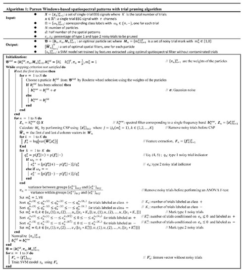
Figure 2.
Proposed PWSPTP algorithm.
2.4. Mixture of Expert Classifiers
It has been determined that a mixture of expert classifiers could improve the classification accuracy [30]. The present study linearly combined multiple classifiers to predict the MI class. Each classifier played the role of one expert and was trained by the features extracted from one spectral filter with bandwidth and one spatial filter . The mixing coefficient of was the importance weight . A support vector machine (SVM) that possessed a strong classification performance [31] was used as the classifier. Note that these classifiers were trained after the spectral and spatial filters were optimized by the PWSPTP and the contaminated trials were removed during the training process. The output of the mixture of expert models was
2.5. Performance Evaluation
To demonstrate the efficiency of discriminative feature extraction of the PWSPTP, this study considered the evaluation protocol of paired binary classification, i.e., left- versus right hand, left hand versus foot, left hand versus tongue, right hand versus foot, right hand versus tongue, and foot versus tongue. This protocol evaluated the discriminative power of the features extracted by the learnt frequency bands when the contaminated trials were eliminated during the training process.
The classification accuracy of the evaluation protocol was the percentage of correctly classified trials. All experiments were conducted with MATLAB (Version R2019a, MathWorks, Natick, MA, USA), with an Intel (R) Core (TM) i7-6900K central processing unit (CPU) @3.2 GHz, a 64 GB random access memory (RAM), and the Microsoft Windows 10 operating system.
3. Experimental Results and Analysis
This section introduced the dataset used in the experiment and then presented the setting of the proposed PWSPTP. The classification results of the PWSPTP were presented when FBCSP and BSSFO are compared. Finally, a discussion is provided to analyze the experimental results.
3.1. Dataset
BCI Competition IV Datasets 2a provided by the Institute for Knowledge Discovery were used for the evaluation of the proposed PWSPTP [32]. Nine subjects performed four MI tasks (left hand, right hand, both feet, and tongue). One training session and one testing session were recorded with 22 EEG channels and were sampled with a frequency of 250 Hz for each subject. Each session consisted of 288 trials with 72 trials for each MI task. The EEG signals in the dataset were originally bandpass filtered (0.5 Hz–100 Hz) and further processed by a 50 Hz notch filter to suppress line noise. This study bandpass filtered (4 Hz–40 Hz) the EEG signals to cover the µ (8–14 Hz) and β (14–30 Hz) rhythms. Although prior neurophysiological knowledge was adopted, there were no predefined frequency bands in the filter bank. A small Laplacian derivation [33] was applied to each electrode using anterior, posterior and both lateral electrodes to increase the signal-to-noise ratio. Following the same protocol as that adopted by [34], the time segment with the length of 2 s between 0.5 s and 2.5 s after visual cue onset in each trial was adopted for MI classification in both training and testing sessions. Detailed descriptions of the BCI Competition IV Datasets 2a could be found in [32].
3.2. Setting of PWSPTP
The initial prior distribution which was adopted to generate a set of particles was set as a mixture of Gaussian functions according to prior neurophysiology knowledge
where µ and β represent the mean frequencies of the µ- (8–14 Hz) and β-rhythms (14–30 Hz), respectively, and the covariance was set to be an identical matrix. Therefore, the start and the end of the frequency band (particle) were initially sampled from the mixture of Gaussians.
The half number of the spatial patterns, d, was set to one. A Gaussian kernel-based SVM was used in the present study owing to its superior classification performance of BCI studies [7,21,35].
3.3. Effects of Numbers of Particles
The number of particles (N) was the hyperparameter of the PWSPTP. To investigate the effects of the hyperparameter to the MI classification accuracy, PWSPTP used various N values were implemented. Figure 3 shows the experimental results with various N values on the left- and right-hand MI classification accuracy for subject 2. The classification accuracy was improved as N increased, but was not monotonically improved when N was larger than 35. Therefore, the PWSPTP was used for the construction of the filter bank with 35 frequency bands.

Figure 3.
Effects of the number of particles on left- and right-hand MI classification accuracy for subject 2. Any data not included between the whiskers are plotted as an outlier with red plus sign.
3.4. Effects of Pruning Percentages
The pruning percentages ( and ) determined the numbers of type-1 and -2 noisy trials and were designed empirically. The previous study revealed that the trial pruning method improved the classification accuracies of the subjects that were associated with low-MI classification accuracies [12]. The left-hand versus right-hand classification of subject 2 has been known as a strongly confused MI binary classification [12,21,36]. The left- and right-hand MI classifications of subject 2 were conducted to analyze the effects of various and , as presented in Figure 4.
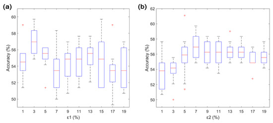
Figure 4.
(a) Effects of pruning percentage of type-1 noisy trial on the left- and right-hand MI classification accuracies for subject 2. (b) Effects of pruning percentage of type-2 noisy trial on left- and right-hand MI classification accuracy for subject 2. Any data not included between the whiskers are plotted as an outlier with red plus sign.
Increasing the values of and improved the classification accuracy when and were smaller than 3% and 7%, respectively. The classification accuracy decreased when and were larger than 3% and 7%, respectively. Therefore, and were empirically set to 3% and 7%, respectively, to remove two types of noisy trials during the training phase.
3.5. Visualization of Spatial Patterns and Distribution of Discriminative Frequency Band
The most significant spatial patterns learnt along with the spectral filter (particle) with maximum importance weight value of subject 1 are shown in Figure 5. These spatial patterns are distinguishable among six MI pairs, and were consistent with the neurophysiological plausibility [5]. The learnt spatial patterns identified the attenuations and increases in the localized neural rhythmic activities and helped improve the MI classification.

Figure 5.
Most significant spatial patterns corresponding to the frequency band (particle) with maximum importance weight value for subject 1 where L, R, F, and G denote left hand, right hand, foot, and tongue, respectively. Red color and blue color represent the highest and lowest values of the spatial patterns, respectively.
The distribution of the discriminative frequency band learnt by the proposed PWSPTP is presented in Figure 6. The probability was computed within an interval of 0.5 Hz. Most optimized particles distributed around the µ-rhythm. This indicates that these discriminative frequency bands matched the neurophysiological knowledge.
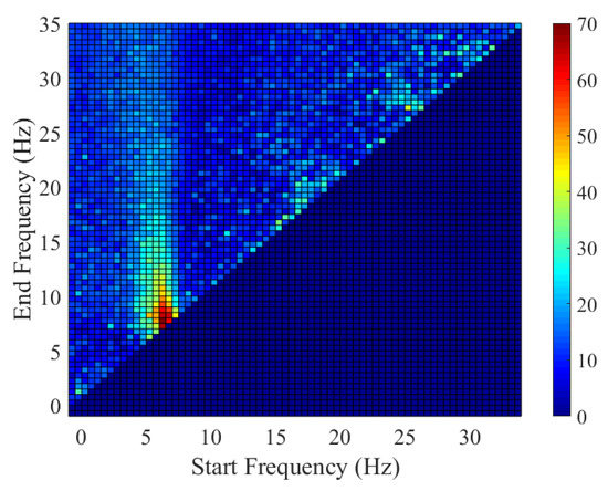
Figure 6.
Visualization of the distribution of the discriminative frequency band wherein the optimized particles were marked as black circles.
3.6. Classification Performance
The classification performance of the PWSPTP was averaged over ten independent runs owing to its stochastic properties. The experimental results of six paired binary MI classifications among nine subjects are presented in Table 1. The classification accuracies varied from subject to subject. Specifically, subjects 1 and 3 obtained higher accuracies, while subject 5 and 6 obtained lower accuracies. For the paired MI classification, the PWSPTP achieved better performance in the MI of the left hand vs. foot, left hand vs. tongue, and right hand vs. tongue (in this order).

Table 1.
Classification performance of the PWSPTP for six paired binary MI classifications among nine subjects. In this case, L, R, F, and G denote left hand, right hand, foot, and tongue respectively, and μ and σ denote mean and standard deviation, respectively. Bold values indicate the highest classification accuracy among the six paired binary MI classifications.
The PWSPTP was compared with the CSP outcomes [6] to evaluate the effects of the spatiospectral filter optimization integrated in the trial pruning method. The experimental results in Table 2 revealed that the proposed PWSPTP outperformed the CSP. The trial pruning improved the classification accuracy based on the removal of the contaminated trials during the optimization of the spatiospectral filter.
Table 2.
Performance comparison with CSP where L, R, F, and G denote left hand, right hand, foot, and tongue respectively, and μ and σ denote the mean and standard deviation, respectively. Bold values indicate the highest classification accuracy among the CSP and PWSPTP.
4. Discussion
4.1. Effect of Number of Particles on the Classification Accuracy
When the number of particles increased, the classification accuracy was not monotonically improved. As the number of particles was small, only few spectral and spatial patterns could be extracted by these particles (frequency bands) that may not possess sufficient discriminative power for the MI tasks. Conversely, as the number of particles was too large, some particles may be resampled from the same particle with high discriminative power. These particles may possess high overlapping portions of frequency bands compared with the other particles. Although these particles possess high discriminative power, these frequency bands may result in highly similar spectral and spatial patterns that do not provide diverse features for training the BCI. Furthermore, the BCI may overfit the training data that possess large dimensional features. Therefore, an appropriate number of particles could not only extract a sufficient number of spectral and spatial patterns, but prevent too many particles being almost identical.
4.2. Effect of Pruning Percentages on the Training Phase
Continuous increases of the and values may prune more trials that may not be contaminated trials. When too many trials are eliminated, the PWSPTP could not learn accurately the spatiospectral filters owing to the small amount of trials available for the training phase. Insufficient data amounts may lead to overfitting issues in the training of the classifier. These results suggested that approximately 3% and 7% of the trials were respectively contaminated by background noise/artifacts and improper MI for subject 2.
4.3. Asymmetrical Spatial Patterns on Left- versus Right-Hand MI Classification
The learnt spatial patterns of the left-hand versus right-hand MI classification addressed neurophysiologically plausible areas. The spatial patterns of the left- and right-hand MIs focus on the right and left motor cortices, respectively. These asymmetrical spatial patterns on left- versus right-hand MI classifications are consistent with the neurophysiological plausibility [5]. This suggested that the PWSPTP could automatically learn MI-related spatial patterns which match neurophysiological evidence. From the distribution of the discriminative frequency band, the PWSPTP could automatically learn the discriminative frequency bands related to the -rhythm without predefining them so that the discriminative spectral features associated with MI could be effectively extracted for classification.
4.4. Effect of Trial Pruning on Paired Binary MI Classification Performance
It has been revealed that the paired binary MI classification of the left-hand vs. foot was better than the left hand vs. right hand among nine subjects. When the subject performed four MI tasks, the likelihood of performing improper left- /right-hand MI may be higher than that of left-hand/foot MI. Therefore, the left- /right-hand MI may result in more type-2 noisy trials than the left-hand/foot MI. Although PWSPTP could prune the contaminated trials, a few type-2 noisy trials may not be eliminated owing to the use of fixed pruning percentages. Thus, the classification accuracy of the left-hand/foot MI was higher than that of the left-hand/right-hand MI.
The CSP is a data-driven method that is sensitive to contaminated trials. The contaminated trials may increase the likelihood of the MI classifier learning spectral–spatial features irrelevant to the MI task, and could thus hamper the MI classification accuracy. The PWSPTP not only integrated trial pruning in the spatiospectral filter optimization, but shared the information of the discriminative power of spectral features to measure the contamination levels of the trials. Comparing with the CSP, the PWSPTP extracted the spatiospectral features without any noted effects on the outcomes from trials conducted in the presence of noise, and then improved the classification accuracy.
5. Conclusions and Future Work
The present study proposed a PWSPTP that constructed a filter bank without predefined frequency bands and without contaminated trials during the training phase. A Parzen window density estimator was applied to measure both the discriminative power of the spatiospectral features and contamination levels of the trials. A set of discriminative spectral filters was learnt by a particle-based approximation technique. Meanwhile, the use of ANOVA F-tests makes the computation of an importance weight of each spectral filter simpler. A set of potentially contaminated trials were removed during the training of classifiers without the effects of artifacts and improper motor imagery. Six paired binary MI classifications among nine subjects were conducted to evaluate the effectiveness of the learnt filter bank and trial pruning. The PWSPTP outperformed the CSP in terms of classification accuracy. The learnt spatial patterns and discriminative frequency bands were approximately consistent with the neurophysiological plausibility. The number of spectral filters and the number of percentages of pruned trials were hyperparameters and should be defined before running the PWSPTP. Future work will be devoted to the adjustment of the number of spectral filters and the number of percentages of pruned trials in the training phase.
Author Contributions
Conceptualization, C.-P.S., S.-H.Y. and Y.-Y.C.; methodology, C.-P.S., S.-H.Y. and Y.-Y.C.; software, C.-P.S., Y.-T.K. and C.-H.K.; validation, C.-P.S., Y.-S.L., Y.-T.K. and C.-H.K.; formal analysis, C.-P.S., S.-H.Y. and Y.-Y.C.; investigation, C.-P.S., S.-H.Y. and Y.-Y.C.; resources, C.-P.S.; data curation, C.-P.S.; writing—original draft preparation, C.-P.S.; writing—review and editing, C.-P.S., S.-H.Y. and Y.-Y.C.; visualization, C.-P.S. and Y.-S.L.; supervision, S.-H.Y. and Y.-Y.C.; project administration, S.-H.Y. and Y.-Y.C.; funding acquisition, S.-H.Y., Y.-C.L. and Y.-Y.C. All authors have read and agreed to the published version of the manuscript.
Funding
This work was financially supported by Ministry of Science and Technology of Taiwan under the contract numbers of MOST 108-2321-B-010-008-MY2, 108-2314-B-303-010, 108-2636-E-006-010, 109-2636-E-006-010 (Young Scholar Fellowship Program), 107-2221-E-010-021-MY2, and 107-2221-E-010-011. We are also grateful for the support from the Headquarters of University Advancement at the National Cheng Kung University that is sponsored by the Ministry of Education, Taiwan. We are grateful for the support from the National Cheng Kung University Hospital, Taiwan.
Conflicts of Interest
The authors declare no conflict of interest.
References
- Pfurtscheller, G.; Neuper, C. Motor imagery and direct brain-computer communication. Proc. IEEE 2001, 89, 1123–1134. [Google Scholar] [CrossRef]
- Palaniappan, R.; Mandic, D.P. Biometrics from brain electrical activity: A machine learning approach. IEEE Trans. Pattern Anal. Mach. Intell. 2007, 29, 738–742. [Google Scholar] [CrossRef] [PubMed]
- Cecotti, H. A self-paced and calibration-less SSVEP-based brain–computer interface speller. IEEE Trans. Neural Syst. Rehabil. Eng. 2010, 18, 127–133. [Google Scholar] [CrossRef] [PubMed]
- Cecotti, H.; Graser, A. Convolutional neural networks for P300 detection with application to brain-computer interfaces. IEEE Trans. Pattern Anal. Mach. Intell. 2011, 33, 433–445. [Google Scholar] [CrossRef]
- Pfurtscheller, G.; da Silva, F.L. Event-related EEG/MEG synchronization and desynchronization: Basic principles. Clin. Neurophysiol. 1999, 10, 1842–1857. [Google Scholar] [CrossRef]
- Ramoser, H.; Muller-Gerking, J.; Pfurtscheller, G. Optimal spatial filtering of single trial EEG during imagined hand movement. IEEE Trans. Rehabil. Eng. 2000, 8, 441–446. [Google Scholar] [CrossRef]
- Lotte, F.; Congedo, M.; Lécuyer, A.; Lamarche, F.; Arnaldi, B. A review of classification algorithms for EEG-based brain–computer interfaces. J. Neural Eng. 2007, 4, R1. [Google Scholar] [CrossRef]
- Blankertz, B.; Tomioka, R.; Lemm, S.; Kawanabe, M.; Muller, K.-R. Optimizing spatial filters for robust EEG single-trial analysis. IEEE Signal Process. Mag. 2008, 25, 41–56. [Google Scholar] [CrossRef]
- Wang, H.; Zheng, W. Local temporal common spatial patterns for robust single-trial EEG classification. IEEE Trans. Neural Syst. Rehabil. Eng. 2008, 16, 131–139. [Google Scholar] [CrossRef] [PubMed]
- Bashashati, A.; Fatourechi, M.; Ward, R.K.; Birch, G.E. A survey of signal processing algorithms in brain–computer interfaces based on electrical brain signals. J. Neural Eng. 2007, 4, R32. [Google Scholar] [CrossRef] [PubMed]
- Blankertz, B.; Kawanabe, M.; Tomioka, R.; Hohlefeld, F.; Müller, K.-R.; Nikulin, V.V. Invariant common spatial patterns: Alleviating nonstationarities in brain-computer interfacing. In Advances in Neural Information Processing Systems; Massachusetts Institute of Technology Press: Cambridge, MA, USA, 2007; pp. 113–120. [Google Scholar]
- Wang, B.; Wong, C.M.; Wan, F.; Mak, P.U.; Mak, P.-I.; Vai, M.I. Trial pruning based on genetic Algorithm for Single-Trial EEG Classification. Comput. Electr. Eng. 2012, 38, 35–44. [Google Scholar] [CrossRef]
- Lemm, S.; Blankertz, B.; Curio, G.; Muller, K.-R. Spatio-spectral filters for improving the classification of single trial EEG. IEEE Trans. Biomed. Eng. 2005, 52, 1541–1548. [Google Scholar] [CrossRef] [PubMed]
- Dornhege, G.; Blankertz, B.; Krauledat, M.; Losch, F.; Curio, G.; Muller, K.-R. Combined optimization of spatial and temporal filters for improving brain-computer interfacing. IEEE Trans. Biomed. Eng. 2006, 53, 2274–2281. [Google Scholar] [CrossRef] [PubMed]
- Tomioka, R.; Müller, K.-R. A regularized discriminative framework for EEG analysis with application to brain–computer interface. Neuroimage 2010, 49, 415–432. [Google Scholar] [CrossRef]
- Wu, W.; Gao, X.; Hong, B.; Gao, S. Classifying single-trial EEG during motor imagery by iterative spatio-spectral patterns learning (ISSPL). IEEE Trans. Biomed. Eng. 2008, 55, 1733–1743. [Google Scholar] [CrossRef]
- Ang, K.K.; Chin, Z.Y.; Zhang, H.; Guan, C. Filter bank common spatial pattern (FBCSP) in brain-computer interface. In Proceedings of the 2008 IEEE International Joint Conference on Neural Networks (IEEE World Congress on Computational Intelligence), Hong Kong, China, 1–8 June 2008; pp. 2390–2397. [Google Scholar]
- Thomas, K.P.; Guan, C.; Lau, C.T.; Vinod, A.P.; Ang, K.K. A new discriminative common spatial pattern method for motor imagery brain–computer interfaces. IEEE Trans. Biomed. Eng. 2009, 56, 2730–2733. [Google Scholar] [CrossRef]
- Zhang, H.; Chin, Z.Y.; Ang, K.K.; Guan, C.; Wang, C. Optimum spatio-spectral filtering network for brain–computer interface. IEEE Trans. Neural Netw. 2010, 22, 52–63. [Google Scholar] [CrossRef]
- Pfurtscheller, G. Graphical display and statistical evaluation of event-related desynchronization (ERD). Electroencephalogr. Clin. Neurophysiol. 1977, 43, 757–760. [Google Scholar] [CrossRef]
- Suk, H.I.; Lee, S.W. A novel Bayesian framework for discriminative feature extraction in Brain-Computer Interfaces. IEEE Trans. Pattern Anal. Mach. Intell. 2013, 35, 286–299. [Google Scholar] [CrossRef]
- Kachenoura, A.; Albera, L.; Senhadji, L.; Comon, P. ICA: A potential tool for BCI systems. IEEE Signal Process. Mag. 2007, 25, 57–68. [Google Scholar] [CrossRef]
- Sannelli, C.; Braun, M.; Müller, K.-R. Improving BCI performance by task-related trial pruning. Neural Netw. 2009, 22, 1295–1304. [Google Scholar] [CrossRef] [PubMed]
- Zames, G.; Ajlouni, N.M.; Ajlouni, N.M.; Ajlouni, N.M.; Holland, J.H.; Hills, W.D.; Goldberg, D.E. Genetic algorithms in search, optimization and machine learning. Inf. Technol. J. 1981, 3, 301–302. [Google Scholar]
- Sarkar, P. Sequential Monte Carlo methods in practice. Technometrics 2003, 45, 106. [Google Scholar] [CrossRef]
- Chen, Y.-W.; Lin, C.-J. Combining SVMs with various feature selection strategies. In Feature Extraction; Springer: Berlin, Germany, 2006; pp. 315–324. [Google Scholar]
- St, L.; Wold, S. Analysis of variance (ANOVA). Chemom. Intell. Lab. Syst. 1989, 6, 259–272. [Google Scholar]
- Parzen, E. On estimation of a probability density function and mode. Ann. Math. Stat. 1962, 33, 1065–1076. [Google Scholar] [CrossRef]
- Kwak, N.; Choi, C.-H. Input feature selection by mutual information based on Parzen window. IEEE Trans. Pattern Anal. Mach. Intell. 2002, 24, 1667–1671. [Google Scholar] [CrossRef]
- Jacobs, R.A.; Jordan, M.I.; Nowlan, S.J.; Hinton, G.E. Adaptive mixtures of local experts. Neural Comput. 1991, 3, 79–87. [Google Scholar] [CrossRef]
- Burges, C.J. A tutorial on support vector machines for pattern recognition. Data Min. Knowl. Discov. 1998, 2, 121–167. [Google Scholar] [CrossRef]
- Brunner, C.; Leeb, R.; Müller-Putz, G.; Schlögl, A.; Pfurtscheller, G. BCI Competition 2008—Graz Data Set A; Institute for Knowledge Discovery (Laboratory of Brain-Computer Interfaces), Graz University of Technology: Graz, Austria, 2008; pp. 136–142. [Google Scholar]
- Hjorth, B. An on-line transformation of EEG scalp potentials into orthogonal source derivations. Electroencephalogr. Clin. Neurophysiol. 1975, 39, 526–530. [Google Scholar] [CrossRef]
- Ang, K.K.; Chin, Z.Y.; Wang, C.; Guan, C.; Zhang, H. Filter bank common spatial pattern algorithm on BCI competition IV datasets 2a and 2b. Front. Neurosci. 2012, 6, 39. [Google Scholar] [CrossRef]
- Garcia, G.; Ebrahimi, T.; Vesin, J. Support Vector EEG Classification in the Fourier and Time-Frequency Correlation. In Proceedings of the IEEE-EMBS First International Conference on Neural Engineering 2003, Capri Island, Italy, 20–22 March 2003; pp. 591–594. [Google Scholar]
- Lee, K.Y.; Kim, S. Designing discriminative spatial filter vectors in motor imagery brain–computer interface. Int. J. Imaging Syst. Technol. 2013, 23, 147–151. [Google Scholar] [CrossRef]
© 2020 by the authors. Licensee MDPI, Basel, Switzerland. This article is an open access article distributed under the terms and conditions of the Creative Commons Attribution (CC BY) license (http://creativecommons.org/licenses/by/4.0/).