Article

Construction of Analytic Solution to Axisymmetric Flow and Heat Transfer on a Moving Cylinder

by
Vasile Marinca
1 and
Nicolae Herisanu
1,2,*
1
Center for Fundamental Technical Research, Romanian Academy, 300222 Timisoara, Romania
2
Faculty of Mechanics, University Politehnica Timisoara, 300222 Timisoara, Romania
*
Author to whom correspondence should be addressed.
Symmetry 2020, 12(8), 1335; https://doi.org/10.3390/sym12081335
Submission received: 19 July 2020 / Revised: 5 August 2020 / Accepted: 7 August 2020 / Published: 10 August 2020
(This article belongs to the Special Issue Asymptotic Methods in the Mechanics and Nonlinear Dynamics)

Abstract

:
Based on a new kind of analytical approach, namely the Optimal Auxiliary Functions Method (OAFM), a new analytical procedure is proposed to solve the problem of the annular axisymmetric stagnation flow and heat transfer on a moving cylinder with finite radius. As a novelty, explicit analytical solutions were obtained for the considered complex problem. First, the Navier–Stokes equations were simplified by means of similarity transformations that depended on different parameters and some combinations of these parameters, and the problem under study was reduced to six nonlinear ordinary differential equations with six unknowns. The OAFM proves to be a powerful tool for finding an accurate analytical solution for nonlinear problems, ensuring a fast convergence after the first iteration, even if the small or large parameters are absent, since the determination of the convergence-control parameters is independent of the magnitude of the coefficients that appear in the nonlinear differential equations. Concerning the main novelties of the proposed approach, it is worth mentioning the presence of some auxiliary functions, the involvement of the convergence-control parameters, the construction of the first iteration and much freedom to select the procedure for determining the optimal values of the convergence-control parameters.

1. Introduction

It is known that analytical techniques play a very important role in the solution of real-world problems. Most of the engineering problems are modelled by nonlinear partial differential equations or nonlinear ordinary differential equations. In the last years, much attention has been devoted to using and developing new methods to determine approximate analytical solutions of nonlinear equations that appear in the study of Newtonian or non-Newtonian fluids. The investigation of axisymmetric flow is of great significance in engineering and industrial processes. For instance, Gorla [1] was concerned with the boundary layer flow of laminar incompressible fluid in the vicinity of an axisymmetric stagnation point for a variation with time of the free stream on a circular cylinder. The unsteady viscous flow in the vicinity of an axisymmetric stagnation point of an infinite cylinder was investigated by Takhar et al. [2], when the free stream velocity and the velocity of the cylinder varied arbitrarily with time. Furthermore, the self-similar solution was obtained when the velocity of the cylinder and the free stream velocity varied inversely as a linear function of time. Laminar stagnation flow, axisymmetrically and obliquely impinging on a generator of a circular cylinder, was formulated by Widman and Putkaradze [3] as an exact solution of the Navier–Stokes equations. The outer stream was composed of a rotational axial flow superposed onto an irrotational radial stagnation flow normal to a cylinder. Revnic et al. [4] studied the steady axisymmetric stagnation flow and heat transfer on a thin infinite cylinder in the cases of constant wall temperature and constant wall heat flux. An analytic solution for the flow of a second-grade fluid over of a radially stretching sheet was presented by Ahmad et al. [5] in the form of a series. The stagnation flow in the annular domain between two cylinders was studied by Hong and Wang [6]. Fluid was injected in wand radially from a fixed outer cylinder towards and axially translating and rotating an inner cylinder like the convective cooling of a moving rod. Hayat and Nawaz [7] considered the MHD flow analysis of a viscous fluid between two radially stretching sheets. The fluid was electrically conducting, the sheets were not conducting and an incompressible fluid saturated the porous medium. A system of two singular equations was presented by Doo et al. [8] and the equivalence between the 3D axisymmetric inviscid stagnation flows related to Navier–Stokes equations was established. Nadeem et al. [9] discussed the axisymmetric stagnation flow of a micro-polar nanofluid in a moving cylinder with heat transfer. Shahzadet al. [10] reported an exact solution for the axisymmetric two-dimensional flow and heat transfer of an elastically conducting viscous fluid over a nonlinear radially stretching porous sheet within a porous medium. Hayat et al. [11] investigated the heat transfer effects in the axisymmetric flow of an incompressible third-grade fluid between the stretching surfaces. The steady laminar incompressible flow and heat transfer of a viscous fluid between two circular cylinders for two different types of thermal boundary conditions were studied by Mastroberardino [12]. Dual solutions were found for the study of axisymmetric stagnation point flow and heat transfer of a viscous and incompressible fluid due to a permeable moving flat plate with partial sleep by Rosca et al. [13]. The flow of an electrically conducting fluid in the vicinity of an axisymmetric stagnation point on a moving cylinder under the influence of a magnetic field was studied by Hazarika and Sarmah [14], and the normal impingement of the rotational stagnation point on a liquid layer was studied by Weidman [15]. Khanet al. [16] analysed the two-dimensional axisymmetric flow and heat transfer of a modified second-grade fluid over an isothermal nonlinear radially stretching sheet. The unsteady MHD axisymmetric flow of Carreau nanofluid over a radially stretching sheet was investigated by Azamet al. [17].
Nadeemet al. [18] considered the steady MHD flow of nanofluids between two concentric circular cylinders with the consideration of a heat generation/absorption effect. The floor was assessed with respect to constant surface temperature and constant heat flux thermal boundary conditions. Mahapatua and Sidui [19] studied heat transfer in non-axisymmetric Homann stagnation point flows towards a stretching sheet. They showed that, under certain conditions, there is a new family of axisymmetric viscous stagnation point flow depending on the ratios of shear-to-strain rate at the plate.
The main objective of current investigations was to examine the stagnation flow in the annular region between two cylinders with heat transfer using the Optimal Auxiliary Functions Method (OAFM). The Navier–Stokes equations were simplified by means of similarity transformations so that the problem under study was reduced to six nonlinear ordinary differential equations further investigated with the OAFM. The accuracy of the results obtained by our approach was proven by numerical simulations developed to validate analytical approximate solutions. Our procedure was independent of the presence of small or large parameters in the governing equations or initial/boundary conditions, since the determination of the convergence-control parameters was independent of the magnitude of the involved coefficients. The procedure was based on the construction of the linear operators and auxiliary functions in combination with the presence of several initially unknown convergence-control parameters. These parameters were optimally determined by means of rigorous mathematical procedures. New explicit and accurate analytical solutions were finally obtained using only the first iteration, which illustrates the power and efficiency of the proposed approach.

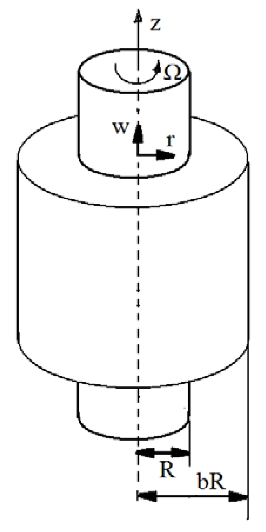
2. Equations of Motion

In this section, we consider steady laminar incompressible flow between two cylinders [5,9]. The vertical inner cylinder of radius R is rotating with angular velocity and is moving with velocity W in the axial z direction. The inner cylinder is enclosed by an outer cylinder of radius bR. The flow isaxisymmetric about the z-axis and the fluid is injected radially with velocity U from the outer cylinder towards the inner cylinder.
In Figure 1 is shown the geometry of the problem. The cylindrical coordinates are (r,θ,z) and the corresponding velocity components are given by (u,v,w).
Supposing that end effects can be ignored, the constant property continuity equation, the constant property Navier–Stokes equations with r, θ and z components of momentum and the energy conservation equations are as follows:
u r + u r + w z = 0
u u r + w u z v 2 r = 1 ρ p r + ν ( 2 u r 2 + 1 r u r u r 2 + 2 u z 2 φ k 0 u ) σ B 0 2 ρ u
u v r + w v z + u v r = ν ( 2 v r 2 + 1 r v r + 2 v z 2 v r 2 )
u w r + w w r = 1 ρ ρ z + ν ( 2 w r 2 + 1 r w r + 2 w z 2 φ k 0 w )
c p ( u T r + w T z ) = λ ρ ( 2 T r 2 + 1 r T r + 2 T z 2 ) + + ν [ 2 ( ( u r ) 2 + u 2 r 2 + ( w z ) 2 ) + ( v r v r ) 2 + ( v z ) 2 + ( u r + w r ) 2 ] + σ B 0 2 ρ u 2
where ρ is the density, p is the pressure, ν is the kinematic viscosity, δ is the electrical conductivity, B0 is the constant magnetic field applied in the z-direction, φ is the porosity, k0 is the permeability of the porous medium, cp is the specific heat, T is the temperature and λ is the thermal diffusivity.
Let us define the following similarity transformations and non-dimensional variables:
u = U f ( η ) η 1 2 , v = Ω R h ( η ) , w = 2 U f ( η ) ξ + W g ( η )
η = r 2 R 2 , ξ = z R 1
Using the above transformations, Equation (1) is automatically satisfied. Supposing that the temperature of the outer cylinder is held constant at Tb and the temperature of the inner cylinder at Ts, and considering the temperature T of the following form:
T ( η ) = T b + ( T s T b ) [ ξ 2 K ( η ) + ξ q ( η ) + s ( η ) ]
then eliminating pressure between Equations (2) and (4), six similarity equations are derived from Equations (2)–(5) and (8):
η f ( I V ) ( η ) + 2 f ( I I I ) ( η ) + Re [ f ( η ) f ( I I I ) ( η ) f ( η ) f ( η ) ( M + Φ ) f ( η ) ] = 0
η g ( η ) + g ( η ) + Re [ f ( η ) g ( η ) f ( η ) g ( η ) Φ f ( η ) ] = 0
4 η h ( η ) + 4 h ( η ) h ( η ) η + Re ( 4 f ( η ) h ( η ) + 2 f ( η ) h ( η ) η ) = 0
η K ( η ) + K ( η ) + Re Pr [ f ( η ) K ( η ) 2 f ( η ) K ( η ) ] + 4 Pr E c η f 2 ( η ) + Re Pr E c M f 2 ( η ) = 0
η q ( η ) + q ( η ) + Re Pr [ f ( η ) q ( η ) α g ( η ) K ( η ) ] + 4 α Pr E c η f ( η ) g ( η ) + Re Pr E c M f 2 ( η ) = 0
2 η s + 2 s + K ( η ) + Re Pr [ 2 f ( η ) s ( η ) α g ( η ) q ( η ) ] + Pr E c [ 2 f 2 ( η ) η 2 + 8 f 2 ( η ) 4 f ( η ) f ( η ) η + 2 α 2 η g 2 ( η ) + β 2 ( 2 η h 2 ( η ) 2 h ( η ) h ( η ) + h 2 ( η ) 2 η ) ] + Re Pr E c M f 2 ( η ) = 0
where Re = 1 2 U R ν 1 is the cross flow Reynolds (Re) number, M = σ B 0 2 ρ R is the Hartman number, Φ = ν φ ρ λ R is the porosity parameter, Pr = ν ρ p λ 1 is the Prandl number, E c = U 2 c p ( T s T b ) is the Eckert number and α = W U and β = Ω R U are velocity ratios.
The boundary conditions are no slip on the inner cylinder and uniform injection on the outer cylinder as follows:
f ( 1 ) = 0 , f ( 1 ) = 0 , f ( b ) = b , f ( b ) = 0
g ( 1 ) = 1 , g ( b ) = 0 , h ( 1 ) = 1 , h ( b ) = 0
For the heat problem, the boundary conditions are as follows:
k ( 1 ) = 0 , k ( b ) = 0 , q ( 1 ) = 1 , q ( b ) = 0 , s ( 1 ) = 1 , s ( b ) = 0
In the following section, we develop some approximate solutions using the OAFM.

3. Basics of the Optimal Auxiliary Functions Method (OAFM)

We use the fundamental concept of OAFM developed in [20,21,22] and considering the general nonlinear differential equation
D [ F ( η ) ] + F f ( η ) = 0 , η H
with initial/boundary conditions
B ( F , F η ) = 0
where D is a general differential operator, Ff(η) is an unknown function, H is the domain of interest, B is a boundary operator and F(η) is an unknown function at this stage. In most of the cases, an exact solution for strongly nonlinear equations of types (1) and (2) is hard to find [23].
Supposing that the approximate analytical solution F ˜ ( η ) of Equations (18) and (19) is of the following form:
F ˜ ( η ) = F 0 ( η ) + F 1 ( η , C i ) , i = 1 , 2 , , p
the initial approximation F0(η) and the first approximation F1(η,Ci) are determined as follows. We chosethe initial approximation F0 in order to satisfy the initial/boundary conditions
B ( F 0 , F 0 η ) = 0
and a linear operator L[F(η)] thatsatisfies the following equation:
L [ F 0 ( η ) ] + F f ( η ) = 0
The operator D [ F ( η ) ] can be divided into two parts, namely L and N, where L is the linear operator and N is the nonlinear operator, and therefore Equation (18) can be rewritten in the following form:
L [ F ( η ) ] + N [ F ( η ) ] + F f ( η ) = 0
Inserting Equation (20) into Equation (23), we obtain the following:
L [ F 0 ( η ) ] + L [ F 1 ( η , C i ) ] + N [ F 0 ( η ) + F 1 ( η , C i ) ] + F f ( η ) = 0
Taking into consideration Equation (22), the first approximation F 1 ( η , C i ) is determined from the nonlinear differential equation
L [ F 1 ( η , C i ) ] + N [ F 0 ( η ) + F 1 ( η , C i ) ] = 0
with the corresponding initial/boundary conditions
B ( F 1 ( η , C i ) , F 1 ( η , C i ) η ) = 0
where Ci, i = 1,2,…, p are unknown parameters at this moment.
The nonlinear term which appears into Equation (25) can be expanded as follows:
N [ F 0 ( η ) + F 1 ( η , C i ) ] = n [ F 0 ( η ) ] + k 1 F 1 ( η , C i ) k ! N ( k ) [ F 0 ( η ) ]
To accelerate the convergence of the first approximation F 1 ( η , C i ) and therefore of the approximate solution F ˜ ( η ) , and also to avoid the difficulties that can appear in solving the nonlinear differential Equation (25), we propose another expression such that Equation (25) can be rewritten as follows:
L [ F 1 ( η , C i ) ] + k = 1 p C i f i ( η ) = 0 , B ( F 1 , F 1 η ) = 0
where Ci are arbitrary unknown parameters and fi(η) are functions depending on the initial approximation F0(η), on the functions which appear in N[F0(η)], or are combinations of such expressions. These auxiliary functions fi are very important and are not unique, and it should be emphasized that we have much freedom to choose such auxiliary functions. Using the previous considerations, for instance if F0(η) and N[F0(η)] are polynomial functions, then fi are sums of polynomial functions; if F0(η) and N[F0(η)] are exponential (logarithmic) functions, then fi are sums of exponential (logarithmic) functions, respectively; if F0(η) are trigonometric functions and N[F0(η)] are polynomial functions, then fi are sums of combinations of trigonometric and polynomial functions, and so on. In conclusion, the auxiliary functions are of the same form like F0(η) and N[F0(η)]. In other words, F0(η) and N[F0(η)] are “source” for the auxiliary functions fi.
Now, the unknown parameters Ci can be optimally identified via rigorous methods, and we have much freedom to choose between the last square method, Ritz method, collocation method, Galerkin method, or Kantorowich method or by minimizing the square residual error:
J ( C 1 , C 2 , , C p ) = ( H ) R 2 ( η , C i ) d η , i = 1 , 2 , p
where
R ( η , C i ) = D [ F ( η ) ] + F f ( η )
and F ˜ ( η ) is given by Equations (22), (28) and (29). The values of the parameters Ci are obtained from the following system:
J C 1 = J C 2 = = J C p = 0
In this way, the approximate analytical solution F ˜ ( η ) is well determined after identification of the optimal values of the initial unknown convergence-control parameters Ci.

4. Application of the Optimal Auxiliary Functions Method

We remark that Equation (9) is decoupled from the other equations, and Equations (10) and (11) are decoupled from Equations (12)–(14). At first, we apply the OAFM for Equations (9)–(11). For these equations, the approximate analytic solutions are of the following form:
f ˜ ( η ) = f 0 ( η ) + f 1 ( η , C i )
g ˜ ( η ) = g 0 ( η ) + g 1 ( η , C j )
h ˜ ( η ) = h 0 ( η ) + h 1 ( η , C i )
At this moment, we should emphasize that the linear operator L and the initial approximation F0 given from Equation (22) are not unique. In the following, we present only three possibilities to choose the linear operators and the initial known function Ff(η) for Equations (9)–(11).
Case 4a
L ( f ) = η f ( I V ) + 2 f , F f f ( η ) = 0
L ( g ) = η g + g , F f g ( η ) = 0
L ( h ) = η h + h , F f h ( η ) = 0
Equations (21) and (27) can be rewritten as follows:
L ( f 0 ) = 0 , f 0 ( 1 ) = f 0 ( 1 ) = f 0 ( b ) = 0 , f 0 ( b ) = b
L ( g 0 ) = 0 , g 0 ( 1 ) = 1 , g 0 ( b ) = 0
L ( h 0 ) = 0 , h 0 ( 1 ) = 1 , h 0 ( b ) = 0
From Equations (38)–(40), we obtain the following:
f 0 ( η ) = b [ ( η 1 ) 2 ln b + ( 2 b 2 ) ( η 1 η ln η ) ] ( b 1 ) [ 2 b 2 ( b + 1 ) ln b ]
g 0 ( η ) = 1 ln η ln b
h 0 ( η ) = 1 ln η ln b
Case 4b
L ( f ) = η f ( I V ) , F f f ( η ) = 0
L ( g ) = g , F f g ( η ) = 0
L ( h ) = h , F f h ( η ) = 0
In this case, the initial approximations are as follows:
f 0 ( η ) = b ( b 1 ) 3 ( η 1 ) 2 ( 3 b 1 2 η )
g 0 ( η ) = η b 1 b
h 0 ( η ) = η b 1 b
Case 4c
L ( f ) = f ( I V ) + 2 b 1 f , F f f ( η ) = 8 b ( b 1 ) 5 ( 2 η 3 b + 1 ) e 2 ( b η ) b 1
L ( g ) = g 4 ( b 1 ) 2 g , F f g ( η ) = 4 b e 2 ( b 1 ) 3 e 2 ( b η ) b 1
L ( h ) = h 4 ( b 1 ) 2 h , F f h ( η ) = 4 b e 2 ( b 1 ) 3 e 2 ( b η ) b 1
The initial approximations are obtained in the following form:
f 0 ( η ) = b ( η 1 b 1 ) 2 e 2 ( b η ) b 1
g 0 ( η ) = b - η b - 1 e 2 ( b η ) b 1
h 0 ( η ) = b - η b - 1 e 2 ( b η ) b 1
In what follows, we consider only Case 4a. The nonlinear operators are obtained from Equations (9)–(11), (35)–(37):
N ( f ) = Re [ f f ( I I I ) f f ( M + Φ ) f ] = 0
N ( g ) = Re [ f g f g Φ f ] = 0
N ( f ) = h ( η ) 4 η + Re ( f h + 2 f h 2 η ) = 0
Inserting the initial approximations given by Equations (41)–(43) into Equations (56)–(58), it follows that
N ( f 0 ) = 2 b Re ( b 1 ) 2 [ 2 b 2 ( b + 1 ) ln b ] 2 [ ( 3 b 1 ) ln b 2 ln b + 2 ( b 1 ) 2 η + ln η + 2 2 b η 2 4 ( b 1 ) ln η η + ( 2 b 2 ) ln b + 2 b 2 2 ln 2 b η ] Re ( M + Φ ) b [ 2 η ln b 2 b 2 ( b 1 ) ln η ] ( b 1 ) [ 2 b 2 ( b + 1 ) ln b ]
N ( g 0 ) = b Re ( b 1 ) [ 2 b 2 ( b + 1 ) ln b ] [ ln b + 2 2 b η ln b 2 ( η 1 ) ln η 2 ( b 1 ) ln 2 η ln b + η 2 ( Φ + 1 ) ln b η + 2 b 2 + 2 ( Φ + 1 ) ln b ln b + 2 ( Φ + 1 ) ( b 1 ) ln η ( 2 b 2 ) ln η ln b ]
N ( h 0 ) = ln η 4 η ln b 1 4 η + b Re [ ( η 1 ) 2 ln b + 2 ( b 1 ) ( η 1 η ln η ) ] ( 1 ln η ln b 1 η ln b )
The auxiliary functions corresponding to the first approximation f1(η) from Equation (32) are obtained from Equations (41) and (59):
f i [ 1 η , 1 η 2 , ln η η , ln η , η 2 , η , η ln η , ]
In this way, the first approximation is defined by Equation (28), which becomes the following:
η f 1 ( I V ) + 2 f 1 + C 1 + C 2 η + C 3 η 2 + C 4 η ln η = 0 , f ( 1 ) = f 1 = f 1 ( b ) = f 1 ( b ) = 0
With respect to Equation (63), we can also write the following:
η f 1 ( I V ) + 2 f 1 + C 1 + C 2 η + C 3 ln η + C 4 η + C 5 η 2 = 0
or
η f 1 ( I V ) + 2 f 1 + C 1 η + C 2 η 2 + C 3 η + C 4 η 2 + C 5 ln η η = 0
and so on.
Using only Equation (63), the solution is the following:
f ˜ ( η ) = α η ( 1 ln η ) + β η 2 + γ η + δ 1 12 C 1 η 3 1 72 C 2 η 4 1 240 C 3 η 5 + ( 17 864 η 4 1 72 η 4 ln η ) C 4
where
α = b 1 2 ( b 1 ) ( b + 1 ) ln b [ ( b 1 ) 2 12 C 1 b 3 b 2 b + 1 36 C 2 3 b 4 2 b 3 2 b 2 2 b + 3 240 C 3 + + ( 11 b 3 17 b 2 17 b + 11 432 + b 4 + 2 b 3 36 ( b 1 ) ln b ) C 4 ] β = ln b 2 ( b 1 ) α + b + 1 8 C 1 + b 2 + b + 1 36 C 2 + b 3 + b 2 + b + 1 96 C 3 + [ b 3 ln b 36 ( b 1 ) 7 ( b 2 + b + 1 ) 216 ] C 4 γ = ln b b 1 α b 4 C 1 b 2 + b 18 C 2 b 3 + b 2 + b 48 C 3 + [ b 3 ln b 18 ( b 1 ) + 7 ( b 2 + b ) 108 ] C 4 δ = ln b 2 b + 2 2 ( b 1 ) α + 3 b 1 24 C 1 + 2 b 2 + 2 b 1 72 C 2 + 5 b 3 + 5 b 2 + 5 b 3 480 C 3 + + [ b 3 ln b 36 ( b 1 ) 28 b 2 + 28 b 11 864 ] C 4
The auxiliary functions fi to the first approximations g1 from Equation (33) are the following:
f i [ η , ln η , 1 η , η ln η , ln 2 η , ]
The first approximation g1 is obtained from Equation (28):
g 1 + g 1 + C 5 η + C 6 η 2 + C 7 η ln η + C 8 η ln η = 0 , g ( 1 ) = g 1 ( b ) = 0
such that
g 1 ( η ) = ( 1 η 2 + b 2 1 ln b ln η ) C 5 4 + ( 1 η 3 + b 3 1 ln b ln η ) C 6 9 + + ( b ln b + 2 2 b ln b ln η + 2 η 2 η ln η ) C 7 + ( b 2 ln η + 1 b 2 ln b ln η + η 2 1 η 2 ln η ) C 8 4
Using the methods given above, the first approximation h1 can be obtained from the following:
η h 1 + h 1 + C 9 η + C 10 η 2 + C 11 ln η + C 12 η ln η = 0 , h ( 1 ) = h 1 ( b ) = 0
with the solution as follows:
h 1 ( η ) = ( 1 η 2 + b 2 1 ln b ln η ) C 9 4 + ( 1 η 3 + b 3 1 ln b ln η ) C 10 9 + + ( b ln b + 2 2 b ln b ln η + 2 η 2 η ln η ) C 11 + ( b 2 ln η + 1 b 2 ln b ln η + η 2 1 η 2 ln η ) C 12 4
The approximate analytical solutions of Equations (9)–(11), (15) and (16) are obtained from Equations (32), (33), (41), (42), (66), (70) and (34), (43), (72), respectively:
f ˜ ( η ) = α η ( 1 ln η ) + β η 2 + γ η + δ 1 12 C 1 η 3 1 72 C 2 η 4 1 240 C 3 η 5 + ( 17 864 η 4 1 72 η 4 ln η ) C 4 + f 0 ( η )
where α, β, γ and δ are given by Equation (67).
g ˜ ( η ) = 1 ln η ln b + ( 1 η 2 + b 2 1 ln b ln η ) C 5 4 + ( 1 η 3 + b 3 1 ln b ln η ) C 6 9 + + ( b ln b + 2 2 b ln b ln η + 2 η 2 η ln η ) C 7 + ( b 2 ln η + 1 b 2 ln b ln η + η 2 1 η 2 ln η ) C 8 4
h ˜ ( η ) = 1 ln η ln b + ( 1 η 2 + b 2 1 ln b ln η ) C 9 4 + ( 1 η 3 + b 3 1 ln b ln η ) C 10 9 + + ( b ln b + 2 2 b ln b ln η + 2 η 2 η ln η ) C 11 + ( b 2 ln η + 1 b 2 ln b ln η + η 2 1 η 2 ln η ) C 12 4
For Equations (12)–(14), the linear operator is the same:
L ( K ) = L ( q ) = L ( s ) = L ( x ) = η x + x
and the nonlinear operators are, respectively, as follows:
N ( K ) = Re Pr [ f K 2 f K ] + 4 Pr E c η f 2 + Re Pr E c M f 2
N ( q ) = Re Pr [ f q f q α g k + M E c f 2 ] + 4 α Pr E c η f g
N ( s ) = 1 2 K + Re Pr [ f q f q + 1 2 α g q + 1 2 E c M f 2 ] + + Pr E c [ f 2 η 2 + 4 f 2 2 f f η + α 2 η g 2 + β 2 ( η h 2 h h + h 2 4 η ) ]
The approximate analytical solutions of Equations (12)–(14) are as follows:
K ˜ ( η ) = K 0 ( η ) + K 1 ( η , C i )
q ˜ ( η ) = q 0 ( η ) + q 1 ( η , C j )
s ˜ ( η ) = s 0 ( η ) + s 1 ( η , C i )
where the initial approximations K0, q0 and s0 can be obtained from the following equations:
η K 0 + K 0 = 0 , K 0 ( 1 ) = K 0 ( b ) = 0
η q 0 + q 0 = 0 , q 0 ( 1 ) = q 0 ( b ) = 0
η s 0 + s 0 = 0 , s 0 ( 1 ) = 1 , s 0 ( b ) = 0
Solving Equations (83)–(85), one obtains the following solution:
K 0 ( η ) = q 0 ( η ) = 0 , s 0 ( η ) = 1 ln η ln b
Substituting Equation (86) into Equations (77)–(79), we obtain successively the following:
N ( K 0 ) = b Pr E c ( b 1 ) 2 [ 2 b 2 ( b + 1 ) ln b ] 2 { M Re [ ( η 1 ) 2 ln b + ( 2 b 2 ) ( η 1 - η ln η ) ] 2 + 16 η ( η ln b + 1 b ) 2 }
N ( q 0 ) = λ Pr E c ( b 1 ) 2 [ 2 b 2 ( b + 1 ) ln b ] 2 { M Re [ ( η 1 ) 2 ln b + ( 2 b 2 ) ( η 1 - η ln η ) ] 2 8 α b ( b 1 ) [ 2 b 2 ( b + 1 ) ln b ] ( η ln b + 1 b ) }
N ( K 0 ) = Re Pr b ( b 1 ) [ 2 b 2 ( b + 1 ) ln b ] ln b [ ( η 1 ) 2 η ln b + ( 2 b 2 ) ( 1 1 η ln η ) + + Pr E c b ( b 1 ) 2 [ 2 b 2 ( b + 1 ) ln b ] 2 { [ ( η 1 ) 2 η ln b + ( 2 b 2 ) ( 1 1 η ln η ) ] 2 + 16 [ ( η 1 ) ln b 16 ( b 1 ) ln η ] 2 4 [ ( η 1 ) 2 η ln b + ( 2 b 2 ) ( 1 1 η ln η ) ] [ η 1 ( b 1 ) ln η ] } + α 2 ( η 2 η ln η ln b + η ln 2 η ln b ) + + β 2 ( 4 4 ln η + ln 2 η 4 η ln 2 b + 1 4 η + 2 ln η 2 η ln b ) + Re Pr M E c b [ ( η 1 ) 2 ln b + ( 2 b 2 ) ( η 1 η ln η ) ] 2 ] 2 ( b 1 ) 2 [ 2 b 2 ( b + 1 ) ln b ] 2 }
From Equations (87) and (88), the auxiliary functions fi can be written as follows:
f i [ η 4 , η 3 , η 2 , η , η ln η , η 2 ln η , η 2 ln 2 η , 1 η , ln η , ]
and from Equation (89), these auxiliary functions are as follows:
f i [ η , 1 η , 1 η 2 , η ln η , ln 2 η , η ln 2 η , ln η η , ]
The first approximations K1, q1and s1 are obtained from the following equations:
η K 1 + K 1 + C 13 η + C 14 η 2 + C 15 ln η + C 16 η ln η = 0 , K 1 ( 1 ) = K 1 ( b ) = 0
η q 1 + q 1 + C 17 η + C 18 η 2 + C 19 ln η + C 20 η ln η = 0 , q 1 ( 1 ) = q 1 ( b ) = 0
η s 1 + s 1 + C 21 1 η 2 + C 22 η ln 2 η + C 23 η + C 24 = 0 , s 1 ( 1 ) = s 1 ( b ) = 0
From the above equations, we obtain the following:
K 1 ( η ) = C 13 4 ( 1 η 2 + b 2 1 ln b ln η ) + C 14 9 ( 1 η 3 + b 3 1 ln b ln η ) + + C 15 ( b ln b + 2 2 b ln b ln η + 2 η 2 η ln η ) + C 16 4 ( b 2 ln b b 2 + 1 ln b ln η + η 2 1 η 2 ln η )
q 1 ( η ) = C 17 4 ( 1 η 2 + b 2 1 ln b ln η ) + C 18 9 ( 1 η 3 + b 3 1 ln b ln η ) + + C 19 ( b ln b + 2 2 b ln b ln η + 2 η 2 η ln η ) + C 20 4 ( b 2 ln b b 2 + 1 ln b ln η + η 2 1 η 2 ln η )
s 1 ( η ) = ( 1 1 η b 1 b ln b ln η ) C 21 + ( 3 8 + 2 b 2 ln 2 b 4 b 2 ln b + 3 b 2 3 8 ln b ln η 2 η 2 ln 2 η 4 η 2 ln η + 3 η 2 8 ) C 22 + ( 1 η 2 4 + b 2 1 4 ln b ln η ) C 23 + ( 1 η + b 1 ln b ln η ) C 24
The approximate analytical solutions of Equations (12)–(14) are, respectively, as follows:
K ˜ ( η ) = C 13 4 ( 1 η 2 + b 2 1 ln b ln η ) + C 14 9 ( 1 η 3 + b 3 1 ln b ln η ) + + C 15 ( b ln b + 2 2 b ln b ln η + 2 η 2 η ln η ) + C 16 4 ( b 2 ln b b 2 + 1 ln b ln η + η 2 1 η 2 ln η )
q ˜ ( η ) = C 17 4 ( 1 η 2 + b 2 1 ln b ln η ) + C 18 9 ( 1 η 3 + b 3 1 ln b ln η ) + + C 19 ( b ln b + 2 2 b ln b ln η + 2 η 2 η ln η ) + C 20 4 ( b 2 ln b b 2 + 1 ln b ln η + η 2 1 η 2 ln η )
s ˜ ( η ) = 1 ln η ln b + ( 1 1 η b 1 b ln b ln η ) C 21 + ( 3 8 + 2 b 2 ln 2 b 4 b 2 ln b + 3 b 2 3 8 ln b ln η 2 η 2 ln 2 η 4 η 2 ln η + 3 η 2 8 ) C 22 + ( 1 η 2 4 + b 2 1 4 ln b ln η ) C 23 + ( 1 η + b 1 ln b ln η ) C 24

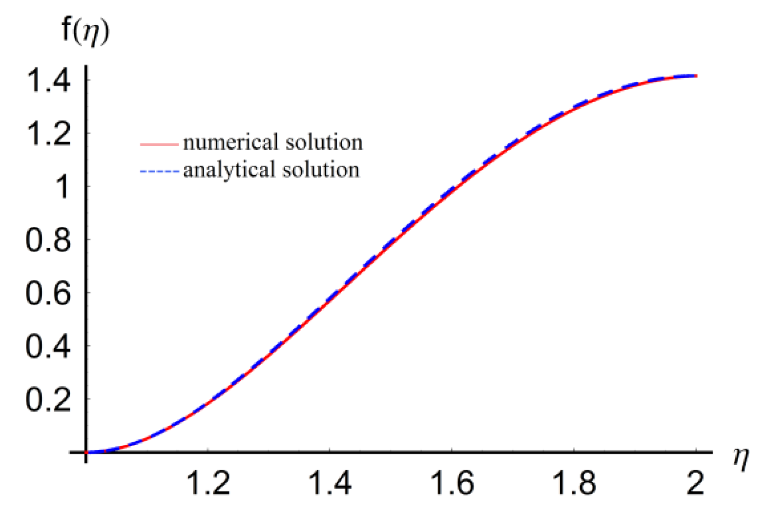
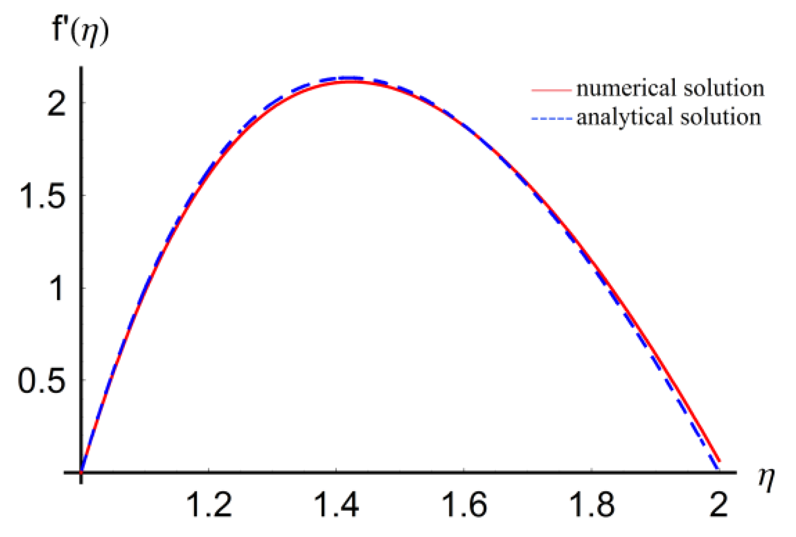
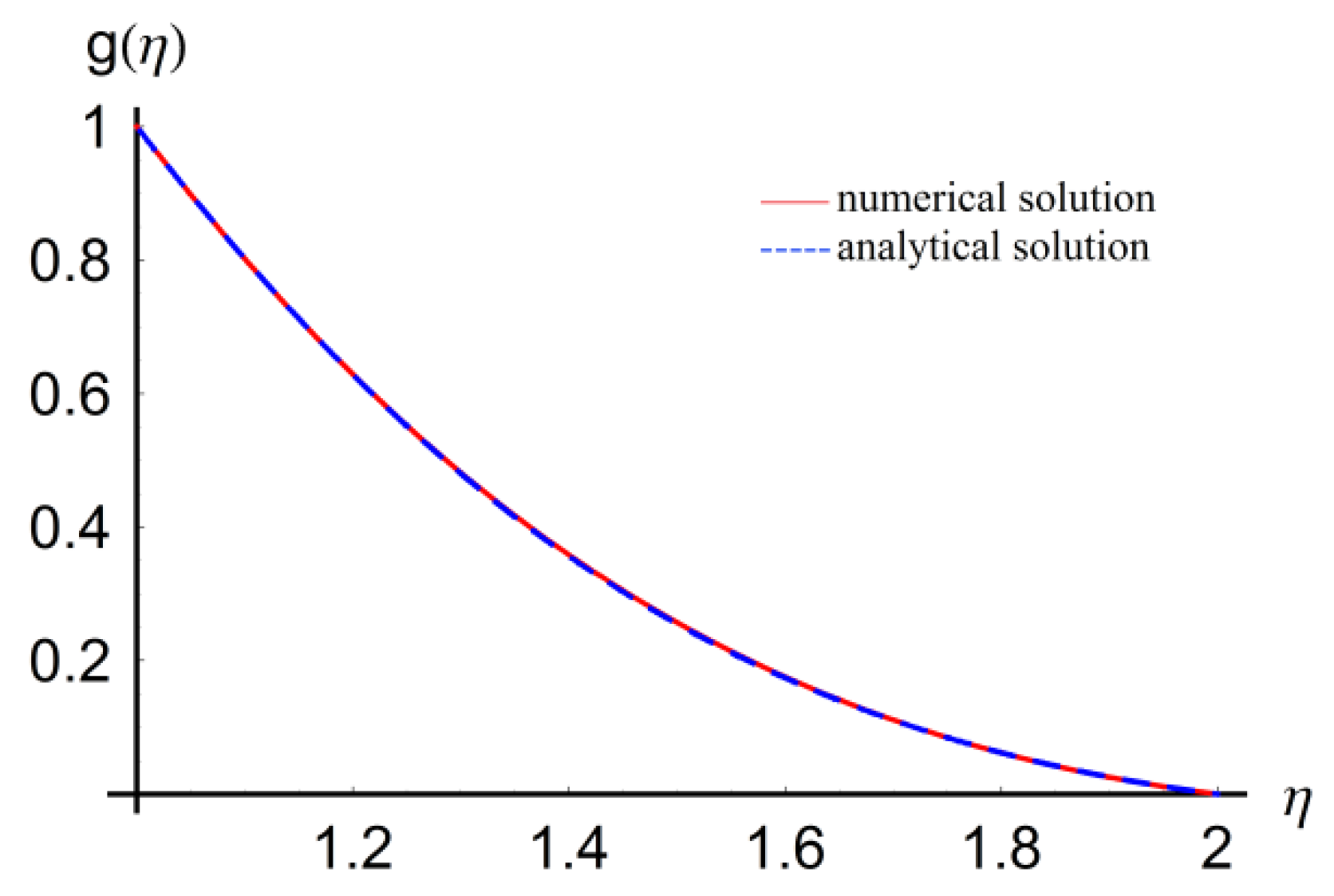
5. Numerical Results

In order to emphasize the effectiveness of the method and to prove the accuracy of the obtained results, we considered a specific set of numerical values for the physical parameters involved in the governing equations, i.e., b = 2, Ec = 0.1, M = 1, Φ = 1, α = 1, β = 1 and Pr = 0.7. Moreover, in order to investigate the influence of the Re number, we considered 3 different Re numbers, namely 1, 4 and 7.
In this situation, following the procedure described for determining the optimal values of the convergence-control parameters (which ensure the convergence of the solution), for Re = 1 we obtain the following optimal values using the collocation method:
C 1 = 1403.5606580130336 , C 2 = 804.2283347147892 , C 3 = 599.9275548052959 , C 4 = 1871.8001233771774 , C 5 = 325.6753295253647 , C 6 = 67.77144388196257 , C 7 = 543.8963537244399 , C 8 = 89.43063711778753 , C 9 = 161.23249058301138 , C 10 = 34.84776686951173 , C 11 = 259.5686396395336 , C 12 = 43.73424584471891 C 13 = 384.08384057024324 , C 14 = 347.15205596692687 , C 15 = 744.3978622088022 , C 16 = 832.622899026811 , C 17 = 22.878035371196603 , C 18 = 15.424368137434392 , C 19 = 67.67949004152135 , C 20 = 44.871875430381564 , C 21 = 18.35411789181781 , C 22 = 8.203667057969469 , C 23 = 22.283213322660515 , C 24 = 40.41496454921898
Taking into account the above values of the convergence-control parameters, the approximate solutions of the similarity functions f, g and h as well as the approximate solutions of the velocity profiles f′, g′ and h′ are graphically presented in Figure 2, Figure 3, Figure 4, Figure 5, Figure 6 and Figure 7 in comparison with corresponding numerical integration results obtained using a fourth-order Runge–Kutta method combined with a shooting approach. This comparison emphasizes the accuracy of the proposed solutions obtained through the OAFM. Moreover, in Figure 8, Figure 9 and Figure 10, we graphically present the variation of K, q and s, corresponding to the heat transfer problem.
Figure 2, Figure 3, Figure 4, Figure 5, Figure 6, Figure 7, Figure 8, Figure 9 and Figure 10 emphasize a very good accuracy of the proposed approximate results, compared to the numerical integration ones obtained through a fourth-order Runge–Kutta method in combination with a shooting approach.
In order to analyse the influence of the Re number, we graphically present in Figure 11, Figure 12 and Figure 13 the variation of f, g and h for three different values of Re, i.e., Re = 1, Re = 4 and Re = 7.
The effects of the Re number on the velocity profiles are demonstrated in Figure 11, Figure 12 and Figure 13. It was found that an increase in the velocity profile f can be observed with an increase in Re (Figure 11), whereas a decrease in the velocity profiles g and h can be observed with an increase in Re (Figure 12 and Figure 13).
A monotonically increasing behaviour of the similarity function f can be observed in Figure 2, and a monotonically decreasing behaviour of the functions g, h and s can be observed in Figure 4, Figure 6 and Figure 10, while the functions K and q have an arbitrary behaviour (Figure 8 and Figure 9).

6. Conclusions

In this paper, we investigated the problem of the stagnation flow in the annular region between two cylinders with heat transfer by using a new and efficient approach, namely the Optimal Auxiliary Functions Method (OAFM). The Navier–Stokes equations were simplified by means of similarity transformations that depend on different parameters and some combinations of these parameters, and the problem under study was reduced to six nonlinear ordinary differential equations with six unknowns. The model consisting of six nonlinear differential equations was investigated through the OAFM. Numerical developments proved that the analytical results obtained using the OAFM are in very good agreement with numerical results obtained by using a fourth-order Runge–Kutta method combined with a shooting approach, which validates the proposed method of solution and the obtained results. The effects of the Re number on the velocity profiles were demonstrated and the behaviour of the solutions for similarity functions and velocity profiles was emphasized.
The proposed procedure is completely different in comparison with any other techniques known in the literature. Some new and remarkable features of the proposed solution approach, which leadsto excellent results, could be emphasized, such as the presence of some auxiliary functions, the involvement of the convergence-control parameters that are initially unknown, the construction of the first iteration and much freedom to select the procedure for the optimal determination of the values of convergence-control parameters.
As a novelty, in comparison with other procedures known in the literature, every nonlinear differential equation in the proposed procedure is reduced to two linear differential equations and the construction of these two linear differential equations is not unique. We have much freedom to choose the auxiliary functions (specific to our approach), which contain some convergence-control parameters. The auxiliary functions depend on the initial approximation and on some terms from the nonlinear operator, while the convergence-control parameters, which are in fact the key of the solution, lead to a high precision since their values are optimally determined using rigorous mathematical procedures. The accuracy of the results obtained using the proposed approach increases as the number of the convergence-control parameters increases. As a consequence of these novel aspects, new explicit and accurate analytical solutions are obtained to annular axisymmetric stagnation flow and heat transfer on a moving cylinder with finite radius using the OAFM. To the best of the authors’ knowledge, this is for the first time when such explicit analytical solutions are presented for the investigated problem.
It is noteworthy that the applicability and efficiency of the proposed approach do not depend on the presence of small or large parameters in the governing equations or in the initial/boundary conditions, because the determination of the convergence-control parameters is independent of the magnitude of the coefficients that appear in the nonlinear differential equations. The optimal values of the initially unknown convergence-control parameters are rigorously determined, and the first iteration ensures very accurate results. The possibility of optimally controlling the convergence of the solutions by means of the auxiliary functions makes this method very effective in practice.
Future investigations will be directed to the study of nanoparticle concentration and the variation of microrotation, in which case, obviously, another set of convergence-control parameters will be needed. This is, in fact, the main disadvantage of the proposed method of solution, since in each particular case another set of convergence-control parameters should be determined in order to obtain the solution.

Author Contributions

Conceptualization, V.M. and N.H.; Formal analysis, V.M.; Investigation, V.M. and N.H.; Methodology, V.M. and N.H.; Validation, N.H.; Visualization, N.H.; Writing—Original draft, V.M. and N.H. All authors have read and agreed to the published version of the manuscript.

Funding

This research received no external funding.

Conflicts of Interest

The authors declare no conflict of interest.

References

  1. Gorla, R.S.R. The final approach to steady state in an axisymmetric stagnation flow following a change in free stream velocity. Appl. Sci. Res. 1983, 40, 247–251. [Google Scholar] [CrossRef]
  2. Takhar, H.S.; Chamkhe, A.J.; Neth, G. Unsteady axisymmetric stagnation-point floor of a viscousfluid on a cylinder. Int. J. Eng. Sci. 1999, 37, 1143–1157. [Google Scholar] [CrossRef]
  3. Weidman, P.D.; Putkaradze, V. Axisymmetric stagnation flow obliquely impinging on a circular cylinder. Eur. J. Mech. B Fluids 2003, 22, 123–131. [Google Scholar] [CrossRef]
  4. Resnic, C.; Grosan, T.; Pop, I. Heat transfer in axisymmetric stagnation flow on a thin cylinder. Studia Univ. Babes Bolyai Math. 2008, LIII, 119–125. [Google Scholar]
  5. Ahmed, I.; Sajid, M.; Hayat, T.; Ayub, M. Unsteady axisymmetric flow of a second-grade fluid over a radially stretching sheet. Comp. Math. Appl. 2008, 56, 1351–1357. [Google Scholar] [CrossRef] [Green Version]
  6. Hong, L.; Wang, C.Y. Annular axisymmetric stagnation flow on a moving cylinder. Int. J. Eng. Sci. 2009, 47, 141–152. [Google Scholar] [CrossRef]
  7. Hayat, T.; Nawaz, M. Effect of heat transfer on magnetohydrodynamic axisymmetric flow between two stretching sheets. Z. Naturforsch. 2010, 65, 961–968. [Google Scholar] [CrossRef]
  8. Doo, C.; Huang, S.J.; Zhang, M.J. On 3D axisymmetric invested stagnation point flow related to Navier-Stokes equations. Nonlinear Anal. Forum 2011, 16, 67–75. [Google Scholar]
  9. Nadeem, S.; Rehman, A.; Vajravelu, K.; Lee, J.; Lee, C. Axisymmetric stagnation flow of a micropolarnanofluid in a moving cylinder. Math. Probl. Eng. 2012. [Google Scholar] [CrossRef]
  10. Shahzad, A.; Ali, R.; Khan, M. On the exact solution for axisymmetric flow and heat transfer over a nonlinear radially stretching sheet. Chim. Phys. Lett. 2012, 29, 084705. [Google Scholar] [CrossRef]
  11. Hayat, T.; Shafiq, A.; Alsaedi, A.; Awais, M. MHD axisymmetric flow of third grade fluid between stretching sheets with heat transfer. Comput. Fluids 2013, 36, 103–108. [Google Scholar] [CrossRef]
  12. Mastroberardino, A. Series solutions of annular axisymmetric stagnation flow and heat transfer on moving cylinder. Appl. Math. Mech. 2013, 34, 1043–1054. [Google Scholar] [CrossRef]
  13. Rosca, A.V.; Rosca, N.C.; Pop, I. Axisymmetric stagnation point flow and heat transfer towards a permeable moving flat plate with surface slip condition. Appl. Math. Comput. 2014, 233, 139–151. [Google Scholar]
  14. Hazarika, G.C.; Sarmah, A. Effect of magnetic field on flow near an axisymmetric stagnation point on a moving cylinder. Int. J. Modern Eng. Res. Tech. 2014, 1, 46–54. [Google Scholar]
  15. Weidman, P. Axisymmetric rotational stagnation point flow impinging on a flat liquid surface. Eur. J. Mech. B Fluids 2016, 56, 188–191. [Google Scholar] [CrossRef]
  16. Khan, M.; Rahman, M.; Manzur, M. Axisymmetric flow and heat transfer to a modified second grade fluid over a radially stretching sheet. Results Phys. 2017, 7, 878–889. [Google Scholar] [CrossRef]
  17. Azam, M.; Khan, M.; Alshomrani, A.S. Effects of magnetic field and partial slip on unsteady axisymmetric flow of Caureaunanofluid over a radially stretching surface. Results Phys. 2017, 7, 2671–2682. [Google Scholar] [CrossRef]
  18. Nadeem, A.; Mahmood, A.; Siddique, J.I.; Zhao, L. Axisymmetric magnetohydrodynamic flow of nanofluidunder heat generation/absorption effects. Appl. Math. Sci. 2017, 11, 2059–2087. [Google Scholar]
  19. Mahapatra, T.R.; Sidqui, S. Heat transfer in non-axisymmetric Homanstagnation point flows towards a stretching sheet. Eur. J. Mech. B Fluids 2017, 65, 522–529. [Google Scholar] [CrossRef]
  20. Herisanu, N.; Marinca, V.; Madescu, G.; Dragan, F. Dynamic response of a permanent magnet synchronous generator to a wind gust. Energies 2019, 12, 915. [Google Scholar] [CrossRef] [Green Version]
  21. Herisanu, N.; Marinca, V. An efficient analytical approach to investigate the dynamics of a misaligned multirotor system. Mathematics 2020, 8, 1083. [Google Scholar] [CrossRef]
  22. Marinca, V.; Herisanu, N. Vibration of nonlinear nonlocal elastic column with initial imperfections. Springer Proc. Phys. 2018, 198, 49–56. [Google Scholar]
  23. Marinca, V.; Herisanu, N. Explicit and exact solutions to cubic Duffing and double-well Duffing equations. Math. Comput. Model. 2011, 53, 604–609. [Google Scholar] [CrossRef]
Figure 1. Geometry of the problem: R is the radius of the inner cylinder, bR is the radius of the outer cylinder, Ω is the angular velocity of the inner cylinder and w is the velocity in the axial direction.
Symmetry 12 01335 g001
Figure 2. Comparison between the approximate solution (73) and numerical integration results for f.
Symmetry 12 01335 g002
Figure 3. Comparison between the approximate solution (73) and numerical results for the velocity profile f’.
Symmetry 12 01335 g003
Figure 4. Comparison between the approximate solution (74) and numerical integration results for g.
Symmetry 12 01335 g004
Figure 5. Comparison between the approximate solution (74) and numerical results for the velocity profile g’.
Symmetry 12 01335 g005
Figure 6. Comparison between the approximate solution (75) and numerical integration results for h.
Symmetry 12 01335 g006
Figure 7. Comparison between the approximate solution (75) and numerical results for the velocity profile h’.
Symmetry 12 01335 g007
Figure 8. Comparison between the approximate solution (98) and numerical integration results for K.
Symmetry 12 01335 g008
Figure 9. Comparison between the approximate solution (99) and numerical integration results for q.
Symmetry 12 01335 g009
Figure 10. Comparison between the approximate solution (100) and numerical integration results for s.
Symmetry 12 01335 g010
Figure 11. The influence of the Re number on f.
Symmetry 12 01335 g011
Figure 12. The influence of the Re number on g.
Symmetry 12 01335 g012
Figure 13. The influence of the Re number on h.
Symmetry 12 01335 g013

