A Framework of Modeling Large-Scale Wireless Sensor Networks for Big Data Collection

 , , ,
, , ,  and
and
Abstract
1. Introduction
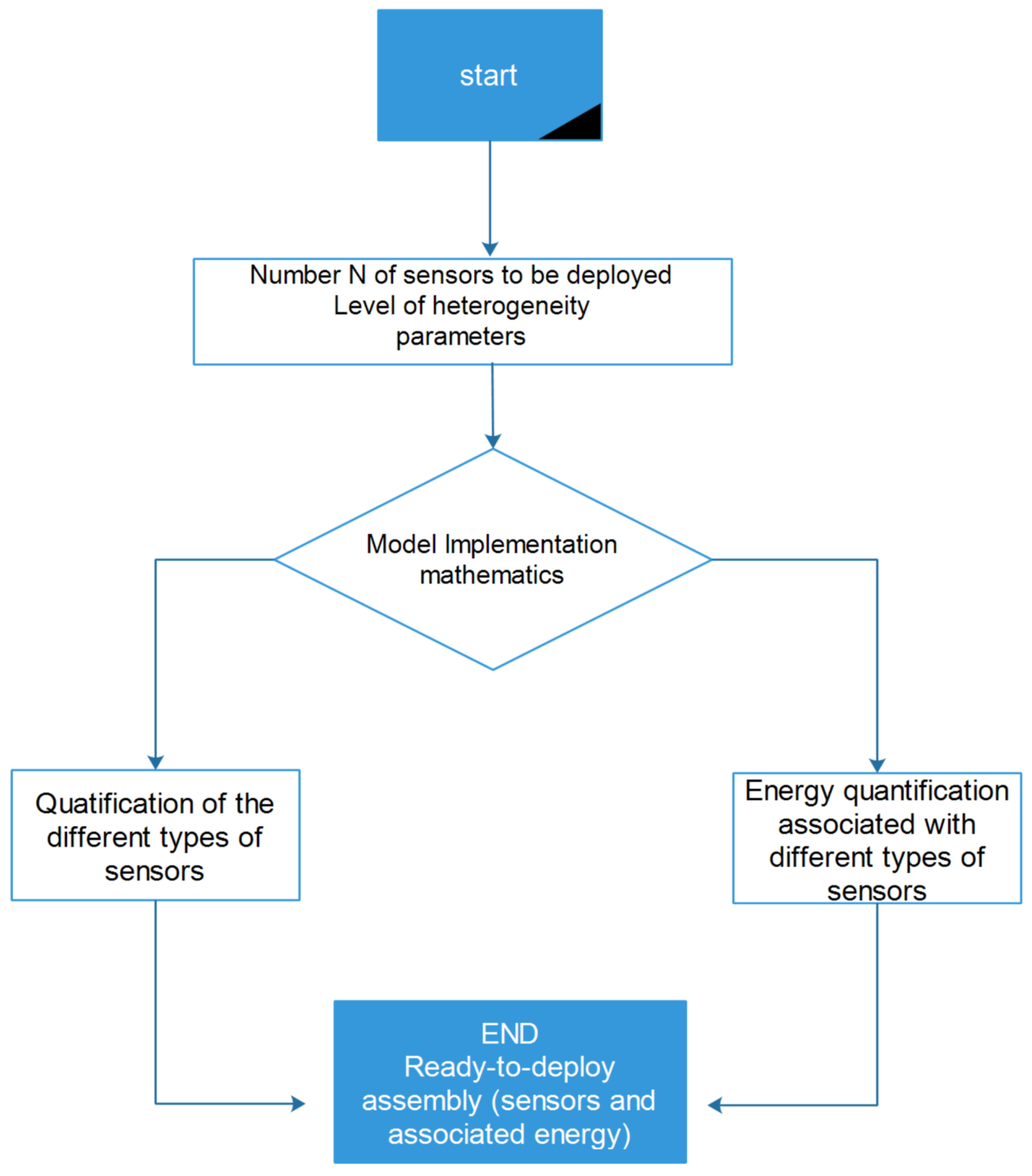
- Proposal of a computation model that determines a set of sensors N and the level of heterogeneity as well as the respective number of the different types of sensors to be used;
- Proposal for a multi-level architecture of LS-WSN that optimizes connectivity and the sensor’s energy consumption;
- Implementation of an algorithm for building clusters of our architecture;
- Proposal for a pre-established routing mechanism in which routing paths are less costly in terms of power consumption;
- Simulation of our proposed LS-WSN model.
2. Big Data, Dimensions and Analysis Tools Related to WSNs
3. Model for Quantifying the Sensors of a Heterogeneous LS-WSN
3.1. Network Assumptions
- Initially, all wireless sensors have the same characteristics instead of the energy supply that is different from a wireless sensor to another. Moreover, each wireless sensor is identified by a unique identifier ID and it is assumed that all sensors are stationary after the network deployments.
- The WSN is heterogeneous.
- The sensors do not know their location, i.e., they are not equipped with a GPS or an antenna.
- The sensors are left unattended after deployment, which means that it is impossible to recharge the sensor’s battery.
- There is a unique stationary base station (BS) that has a stable power supply.
- Each CH performs data aggregation.
- The distances among the sensors are calculated on the basis of the received signal strength. Indeed, when travel toward the receiver, the transmitted signal is attenuated. According to Farooq-i-Azam and Ayyaz [33], this distance is calculated according to transmitted power signal by the sender sensor, the strength of received power of the signal, and the path loss. More generally, distance calculation based on Received Signal Strenght Indicator (RSSI) saves power and no need to add additional circuits in the sensor device.
- The sensors have the ability to control the transmission energy as a function of the distance from the receiving nodes. The node failure is due to energy depletion. In fact, if the transmission distance is too large, the energy used for the transmission of one bit information is enough. Therefore, instead of transmitting data to a far sensor, a given sensor will prefer to transmit to a near sensor and the last will transmit to near neighbor in the same way until reaching the destination sensor that is far from the sender sensor.
- The energy consumption of the data transmission as well as data reception are similar. This is favored by the wireless radio link.
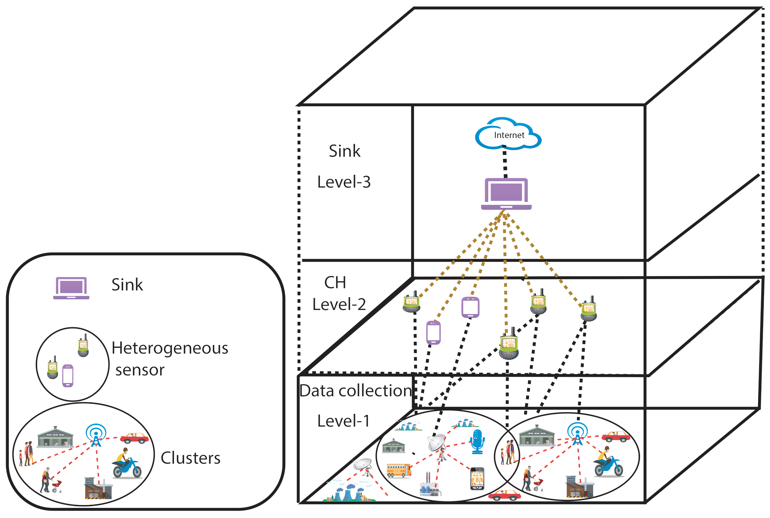
- Sensors randomly equipped in the monitoring area and nodes are indirectly managed by the BS. In fact, according the three-tier architecture presented hereinafter in Figure 5, sensor nodes are led by the cluster heads and the last are managed by the BS.
- Dead sensor IDs are not reused for other sensors.
3.2. Energy Consumption Model
3.3. Network Coverage Model
- Coverage of points in the WSN. Let S be a given area of interest to be monitored. It is said that a sensor covers a point , if and only if:where R is the communication range characterizing each node and defines the Euclidean distance between the nodes u and v.A point is said to be k-covered by a set of k sensors if and only if each of these k sensors covers both the point s, i.e., if and only if:
- Surface coverage in the WSN. The coverage of the surface of an area of interest by a sensor is defined as the total area within the detection range of . Analytically, a surface coverage by a sensor node noted is defined by the formula given in Equation (4).
- Regional coverage in the WSN. Either A a region (zone) or s any point of S. The coverage of region A by a set of sensors is defined analytically by:
3.4. Multilevel Heterogeneous Network Model for LS-WSN
4. Clustering Algorithm for LS-WSNs
4.1. LS-WSN Architecture
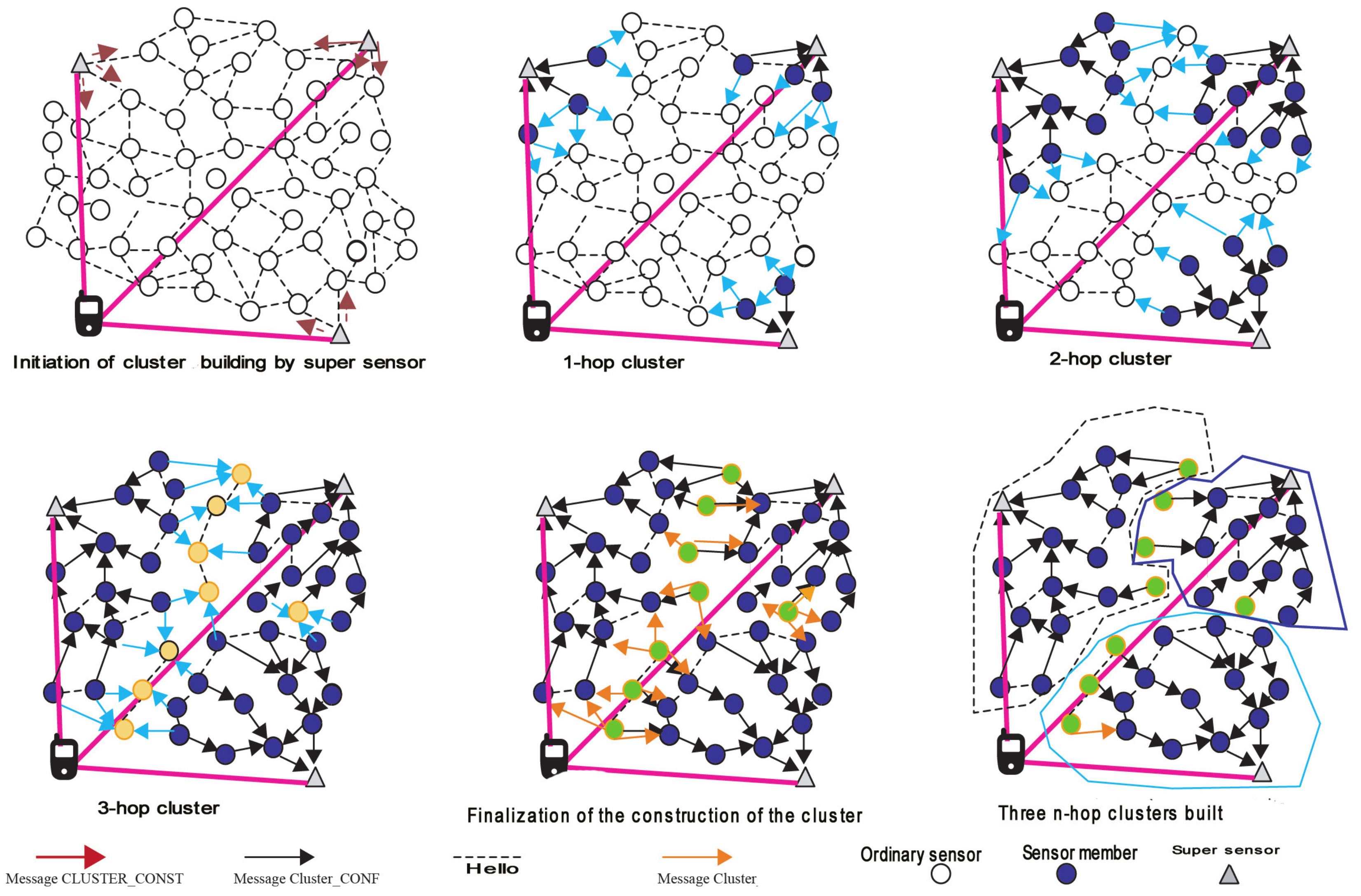
4.2. Cluster Building Algorithm
- Ordinary: initial state of a sensor disconnected from the communication structure.
- Leader: state of a well initiating the construction of its cluster. This is the root of the tree in formation or the CH.
- Member: intermediate node between the root and the leaves of a cluster tree.
- Gateway: intermediate node between clusters.
- Procedure to join a new cluster: The BS periodically sends the list of CHs as well as their locations to the nodes disconnected from the structure (not belonging to a cluster). Each node calculates at each period its distances to the different CHs, if a distance will be R then it sends a “hello” message to the CH concerned. The CH sends him his ID and then the sensor joins the cluster by sending back a message “”.
- Sending information to the BS: Each member node has a standby period T. He wakes up every time, picks up information and sends it to his CH. The CH aggregates the received information and sends the built message to the BS.
- Condition 1: A node receiving two “” messages from the two CHs, chooses the one with the lowest weight.
- Condition 2: A node with a degree of zero (not having neighbors), sends its data directly to the BS and triggers the procedure to join a new cluster’.
- Condition 3: A node leaving its cluster, sends its data to the BS and triggers the procedure to join a new cluster.
| Algorithm 1: Large Scale Wireless Sensor Network (LS-WSN) clustering algorithm |
| Step: 1 After deployment, each sensor sends a “hello” message to the other sensors to allow it to discover its 1-hop neighborhood. Step: 2 Creation and update of the neighborhood table of each sensor node after receiving the “hello” message from its neighborhood. Step: 3 For cluster creation, each CH sends a message “” to the sensor nodes, inviting them to join the cluster they want to build. Step: 4 Upon receipt of the invitations, each sensor node responds with a procedure that we call . This procedure updates the neighborhood table of the ordinary node and decides whether or not to integrate the cluster under construction. Step: 5 Acceptance of the CH invitation. The sensor node becomes a member of the cluster after accepting the message from a CH. The latter then issues a confirmation message at 1-hop to notify the cluster of its membership and to invite its 1-hop neighbors to join it if they have not yet joined a cluster. Step: 6 Upon receipt of the message , depending on the nature of the sensors (CH or sensor node) a procedure is executed.
The management of the procedure. Upon receipt of this message is executed the procedure called depending on the nature of the sensors:
|
5. Results and Discussion
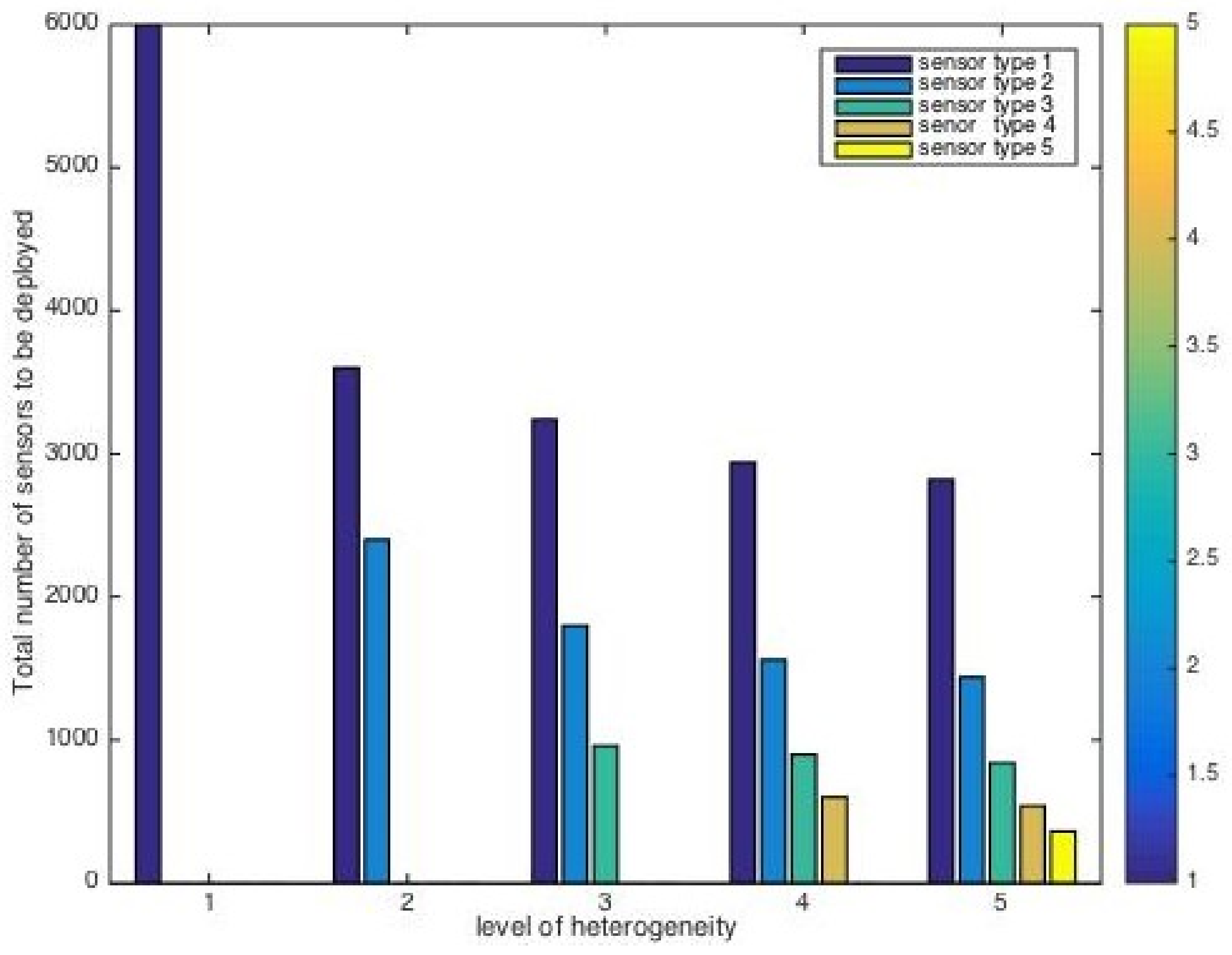
5.1. Evaluation of the Different Sensors of the LS-WSNs
- , the model describes a level-1 heterogeneous network, i.e., it is a homogeneous network using the same kind of sensors. For this network, if we consider sensors to deploy, these sensors will all be of the same type, or sensors of the same nature.
- , the model describes a level-2 heterogeneous network, it is a heterogeneous network with two types of sensors. For this network, if we consider sensors to deploy, we will have 6000 sensors of type-1 and 4000 sensors of type-2.
- , the model describes a level-3 heterogeneous network, it is a heterogeneous network with three types of sensors. For this network, if we consider sensors to deploy, we will have 5200 sensors of type-1, 3000 sensors of type-2 and 1800 sensor of type-3.
- , the model describes a level-4 heterogeneous network, it is a heterogeneous network with four types of sensors. For this network, if we consider sensors to deploy, the sensors of type-1, type-2, type-3, and type-4 are respectively 4900, 2600, 1500, and 1000 sensors.
- , the model describes a level-5 heterogeneous network, it is a heterogeneous network with four types of sensors. For this network, if we consider sensors to deploy, the sensors of type-1, type-2, type-3, type-4, and type-5 are respectively 4700, 2400, 1400, 900, and 600 sensors.
- , the model describes a level-6 heterogeneous network, it is a heterogeneous network with four types of sensors. For this network, if we consider sensors to deploy, the sensors of type-1, type-2, type-3, type-4, type-5, and type-6 are respectively 4608, 2354, 1320, 806, 533 and 378 sensors.
- LS-WSN-1, i.e., a homogeneous network consisting of a set of sensors of the same type, the initial energy of each of these sensors is J.
- LS-WSN-2, i.e., a heterogeneous network with two types of sensors (type-1, type-2). The energy of these different types is J and J respectively.
- LS-WSN-3, i.e., a heterogeneous network with three types of sensors: type-1, type-2, type-3, their energy is respectively J, J and J.
- LS-WSN-4, i.e., a heterogeneous network with four types of sensors. The energy of sensors of type-1, type-2, type-3 and type-4 is J, J, J and J respectively.
- LS-WSN-5, i.e., a heterogeneous network with five types of sensors. The energy of the sensors of type, type, type, type-4, and type-5 are respectively J, J, J, J and 10 J.
- type-1.
- type-2.
- type-3.
- type-4.
- type-5. .
- type-6. .
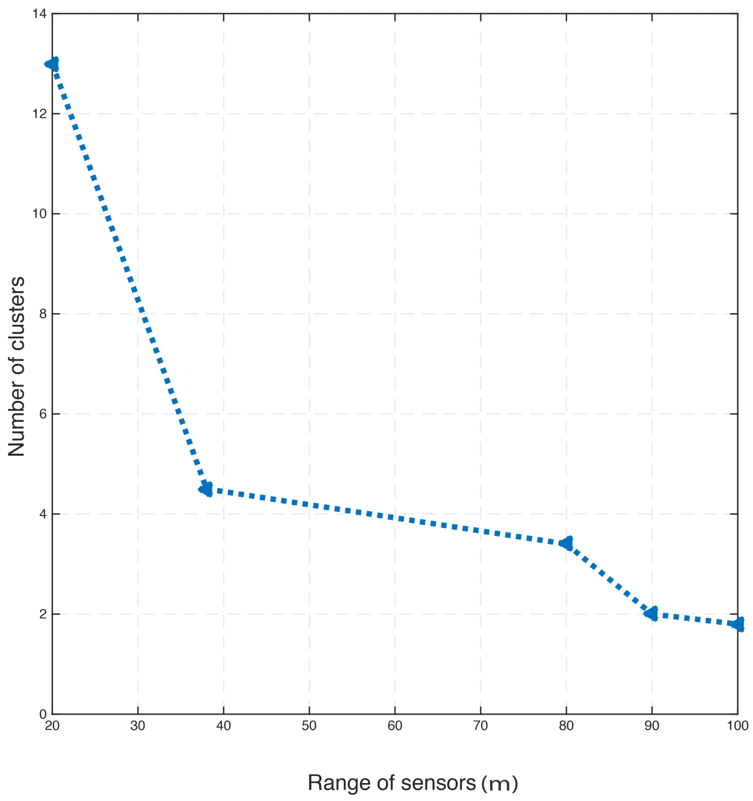
5.2. Evaluation of the Proposed Clustering Algorithm for LS-WSN
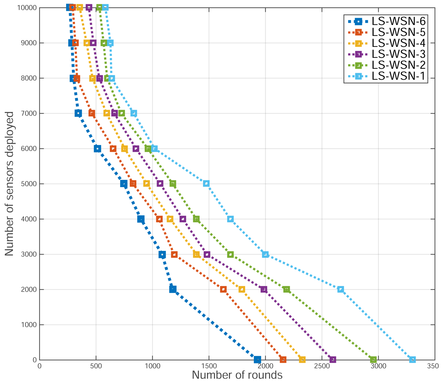
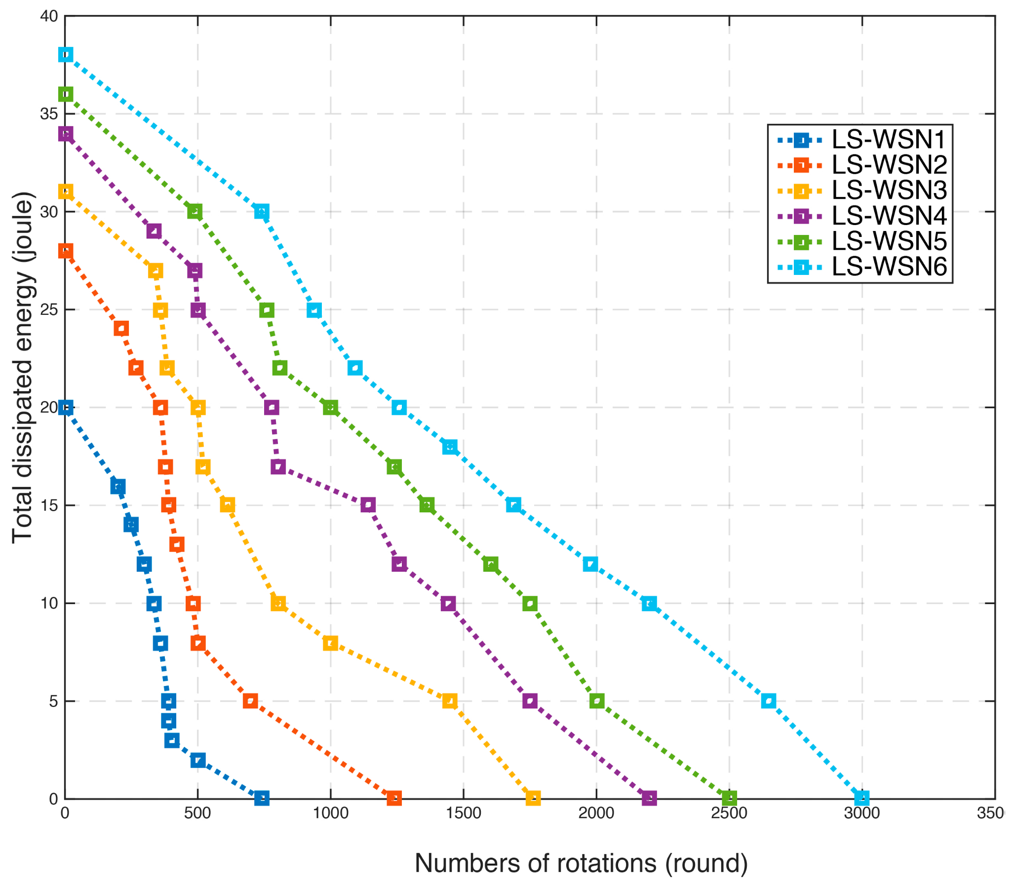
5.2.1. Lifetime
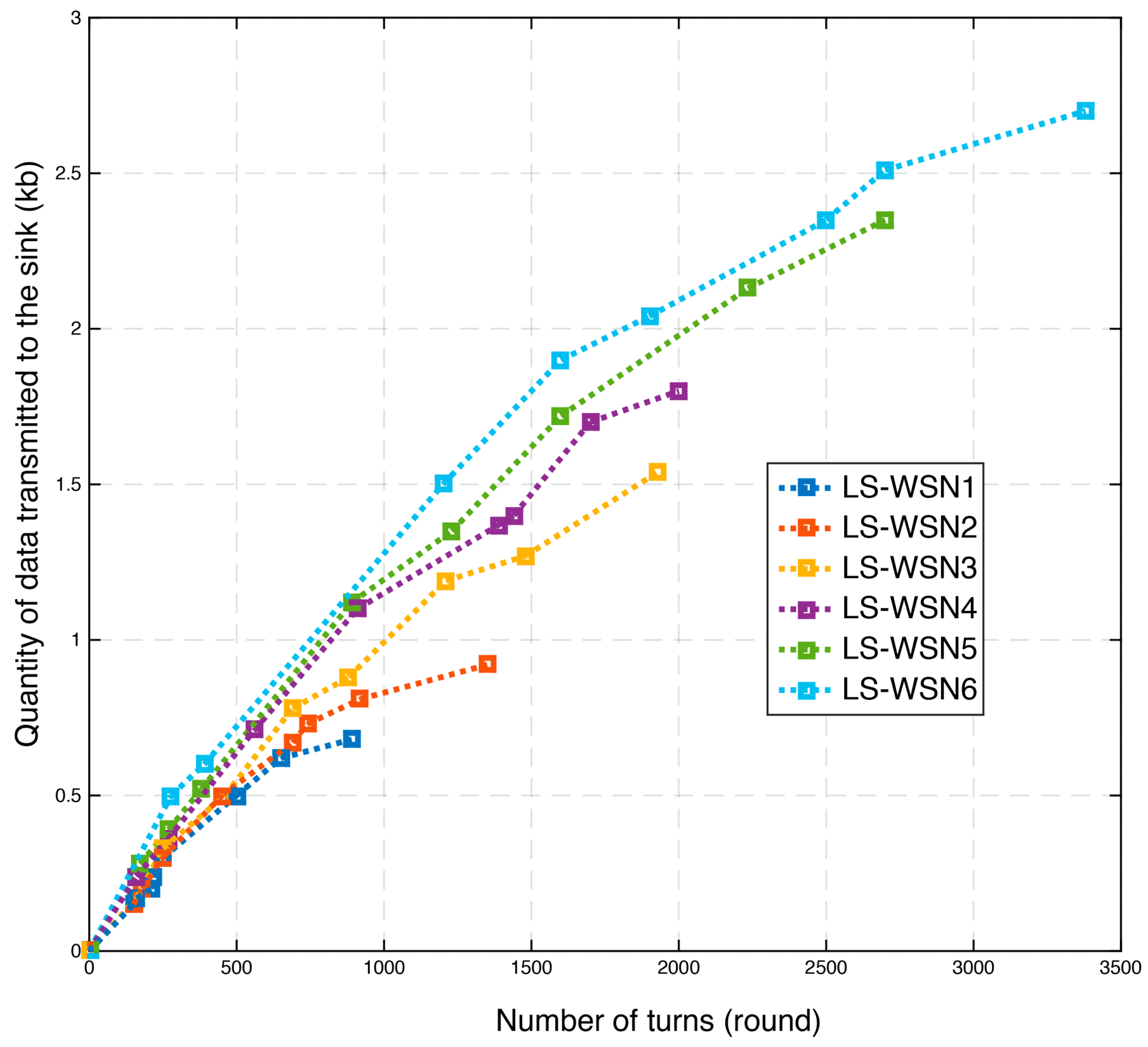
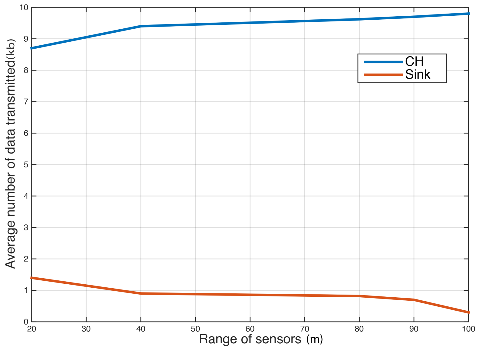
5.2.2. Throughput
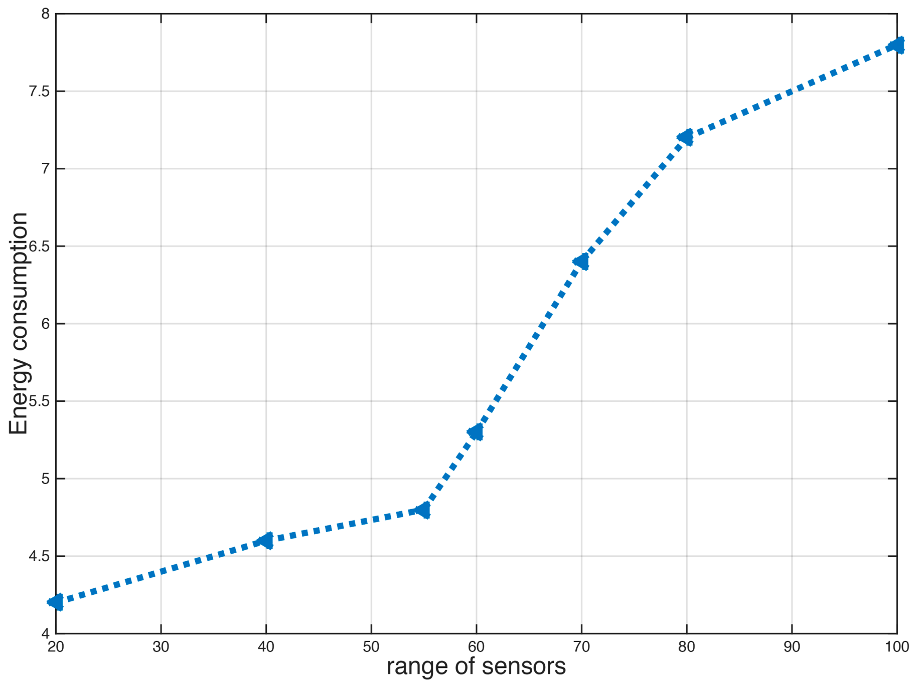
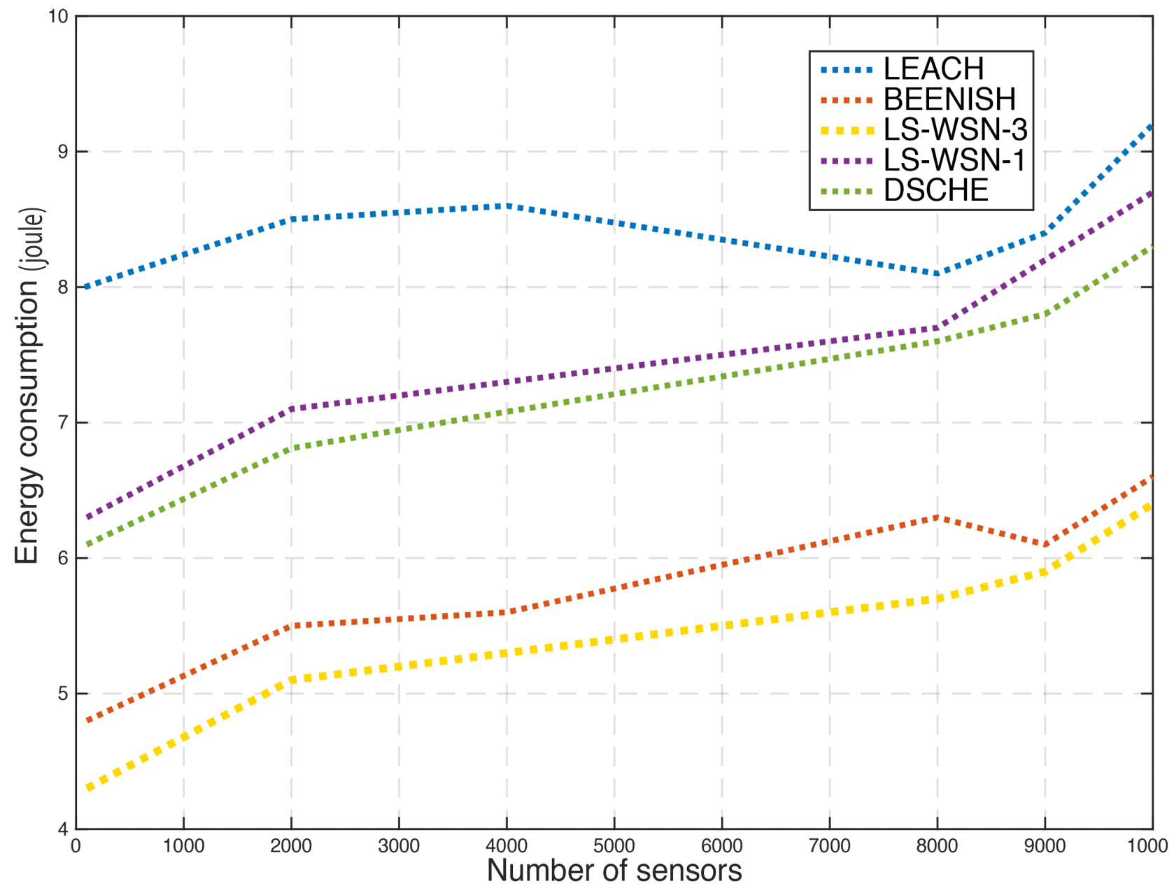
5.2.3. Power Consumption
5.2.4. Effect of Clustering in the Energy Consumption
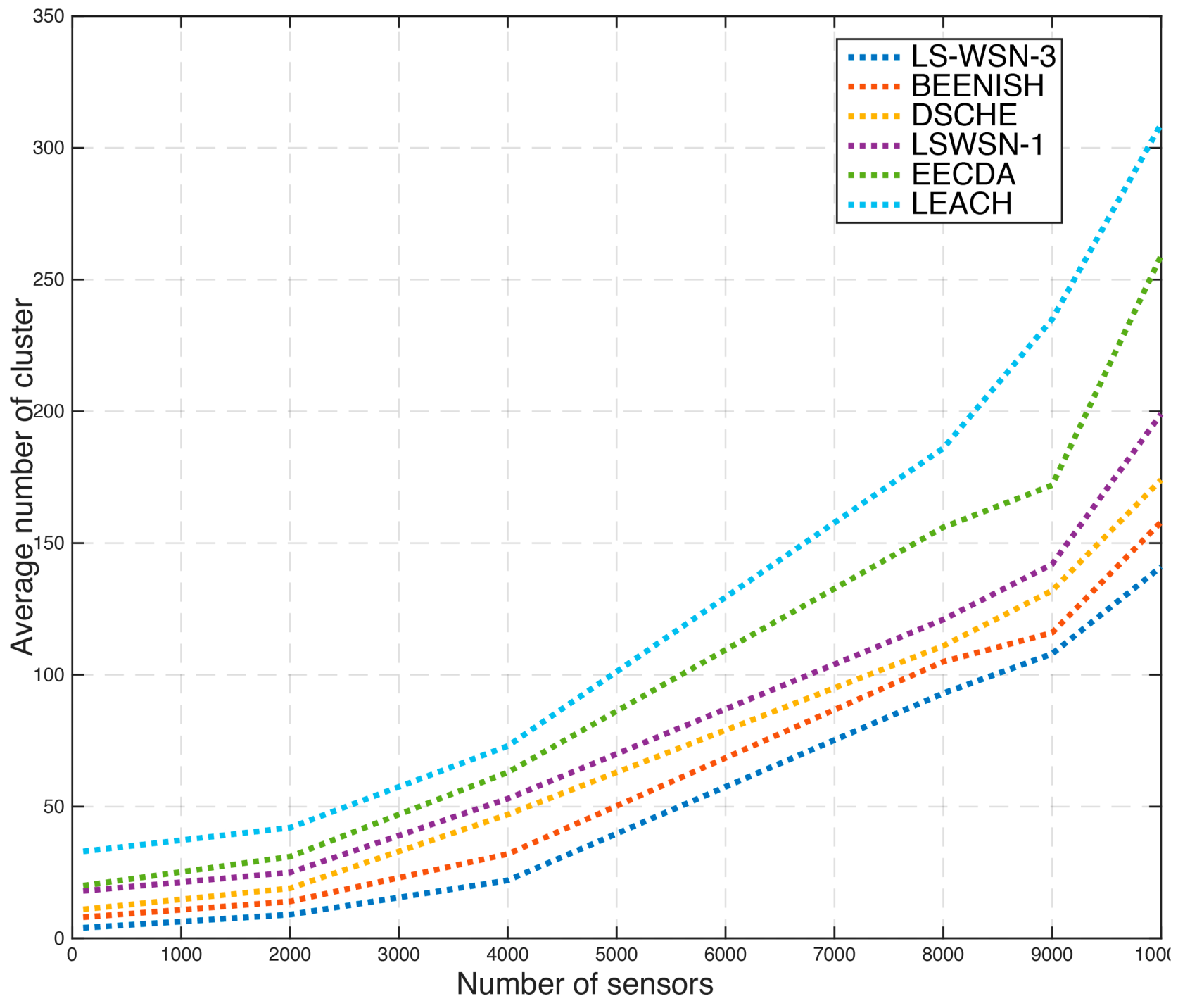
5.3. Performance Comparison
6. Conclusions
Author Contributions
Funding
Acknowledgments
Conflicts of Interest
References
- Djedouboum, A.; Ari, A.A.A.; Gueroui, A.; Mohamadou, A.; Aliouat, Z. Big Data Collection in Large-Scale Wireless Sensor Networks. Sensors 2018, 18, 4474. [Google Scholar] [CrossRef] [PubMed]
- Ari, A.A.A.; Gueroui, A.; Titouna, C.; Thiare, O.; Aliouat, Z. Resource allocation scheme for 5G C-RAN: A Swarm Intelligence based approach. Comput. Netw. 2019, 165, 106957. [Google Scholar] [CrossRef]
- Martínez-de Dios, J.R.; de San Bernabé, A.; Viguria, A.; Torres-González, A.; Ollero, A. Combining unmanned aerial systems and sensor networks for earth observation. Remote Sens. 2017, 9, 336. [Google Scholar] [CrossRef]
- Gbadouissa, J.E.Z.; Ari, A.A.A.; Titouna, C.; Gueroui, A.M.; Thiare, O. HGC: HyperGraph based Clustering scheme for power aware wireless sensor networks. Future Gener. Comput. Syst. 2020, 105, 175–183. [Google Scholar] [CrossRef]
- Baker, T.; Aldawsari, B.; Asim, M.; Tawfik, H.; Maamar, Z.; Buyya, R. Cloud-SEnergy: A bin-packing based multi-cloud service broker for energy efficient composition and execution of data-intensive applications. Sustain. Comput. Inform. Syst. 2018, 19, 242–252. [Google Scholar] [CrossRef]
- Statista Research Department. Internet of Things (IoT) Connected Devices Installed Base Worldwide from 2015 to 2025 (In Billions); Statista Research Department, Ss. Cyril and Methodius University in Skopje, Faculty of Computer Science and Engineering: Skopje, North Macedonia, 2020. [Google Scholar]
- Nzegha, A.F.; Fendji, J.L.E.; Thron, C.; Tayou, C.D. Improving Deep Unconstrained Facial Recognition by Data Augmentation. In Implementations and Applications of Machine Learning; Springer: Cham, Switzerland, 2020; pp. 179–195. [Google Scholar]
- Ari, A.A.A.; Gueroui, A.; Labraoui, N.; Yenke, B.O. Concepts and evolution of research in the field of wireless sensor networks. Int. J. Comput. Netw. Commun. 2015, 7, 81–98. [Google Scholar] [CrossRef]
- Kim, B.S.; Kim, K.I.; Shah, B.; Chow, F.; Kim, K.H. Wireless sensor networks for big data systems. Sensors 2019, 19, 1565. [Google Scholar] [CrossRef]
- Aboubakar, M.; Kellil, M.; Bouabdallah, A.; Roux, P. Using Machine Learning to Estimate the Optimal Transmission Range for RPL Networks. In Proceedings of the NOMS 2020-2020 IEEE/IFIP Network Operations and Management Symposium, Budapest, Hungary, 20–24 April 2020; IEEE: New York, NY, USA, 2020; pp. 1–5. [Google Scholar]
- Marrero, D.; Suárez, A.; Macías, E.; Mena, V. Extending the Battery Life of the ZigBee Routers and Coordinator by Modifying Their Mode of Operation. Sensors 2020, 20, 30. [Google Scholar] [CrossRef]
- Gaboitaolelwe, J.; Zungeru, A.M.; Chuma, J.; Ditshego, N.; Semong, T. A Formal Analytical Modeling and Simulation of Wireless Sensor Home Network. Int. J. Intell. Eng. Syst. 2020, 13, 56–68. [Google Scholar]
- Ari, A.A.A.; Damakoa, I.; Gueroui, A.; Titouna, C.; Labraoui, N.; Kaladzavi, G.; Yenké, B.O. Bacterial foraging optimization scheme for mobile sensing in wireless sensor networks. Int. J. Wirel. Inf. Netw. 2017, 24, 254–267. [Google Scholar] [CrossRef]
- Manfreda, S.; McCabe, M.F.; Miller, P.E.; Lucas, R.; Pajuelo Madrigal, V.; Mallinis, G.; Ben Dor, E.; Helman, D.; Estes, L.; Ciraolo, G.; et al. On the use of unmanned aerial systems for environmental monitoring. Remote Sens. 2018, 10, 641. [Google Scholar] [CrossRef]
- Njoya, A.N.; Ari, A.A.A.; Awa, M.N.; Titouna, C.; Labraoui, N.; Effa, J.Y.; Abdou, W.; Gueroui, A. Hybrid Wireless Sensors Deployment Scheme with Connectivity and Coverage Maintaining in Wireless Sensor Networks. Wirel. Pers. Commun. 2020, 112, 1893–1917. [Google Scholar] [CrossRef]
- Sambo, D.W.; Forster, A.; Yenke, B.O.; Sarr, I.; Gueye, B.; Dayang, P. Wireless Underground Sensor Networks Path Loss Model for Precision Agriculture (WUSN-PLM). IEEE Sens. J. 2020, 20, 5298–5313. [Google Scholar] [CrossRef]
- Mészáros, L.; Varga, A.; Kirsche, M. Inet framework. In Recent Advances in Network Simulation; Springer: Cham, Switzerland, 2019; pp. 55–106. [Google Scholar]
- Wu, X.; Zhu, X.; Wu, G.Q.; Ding, W. Data mining with big data. IEEE Trans. Knowl. Data Eng. 2014, 26, 97–107. [Google Scholar]
- Zikopoulos, P.; Eaton, C.; Zikopoulos, P. Understanding Big Data: Analytics for Enterprise Class Hadoop and Streaming Data; McGraw-Hill Osborne Media: New York, NY, USA, 2011. [Google Scholar]
- Bhadani, A.K.; Jothimani, D. Big data: Challenges, opportunities, and realities. In Effective Big Data Management and Opportunities for Implementation; IGI Global: Hershey, PA, USA, 2016; pp. 1–24. [Google Scholar]
- Chen, M.; Mao, S.; Liu, Y. Big data: A survey. Mob. Netw. Appl. 2014, 19, 171–209. [Google Scholar] [CrossRef]
- Harb, H.; Idrees, A.K.; Jaber, A.; Makhoul, A.; Zahwe, O.; Taam, M.A. Wireless sensor networks: A big data source in Internet of Things. Int. J. Sens. Wirel. Commun. Control 2017, 7, 93–109. [Google Scholar] [CrossRef]
- Vijayakumari, R.; Kirankumar, R.; Rao, K.G. Comparative analysis of google file system and hadoop distributed file system. Int. J. Adv. Trends Comput. Sci. Eng. 2014, 3, 553–558. [Google Scholar]
- Farrah, S.; El Manssouri, H.; Ziyati, E.; Ouzzif, M. An approach to analyze large scale wireless sensors network data. Int. Res. J. Comput. Sci. (IRJCS) 2015, 2, 7–12. [Google Scholar]
- Capriolo, E.; Wampler, D.; Rutherglen, J. Programming Hive: Data Warehouse and Query Language for Hadoop; O’Reilly Media Inc.: Sevastopol, CA, USA, 2012. [Google Scholar]
- Rios, L.G.; Diguez, J.A.I. Big data infrastructure for analyzing data generated by wireless sensor networks. In Proceedings of the 2014 IEEE International Congress on Big Data, Anchorage, AK, USA, 27 June–2 July 2014; IEEE: New York, NY, USA, 2014; pp. 816–823. [Google Scholar]
- Hamidouche, R.; Aliouat, Z.; Ari, A.A.A.; Gueroui, M. An efficient clustering strategy avoiding buffer overflow in IoT sensors: A bio-inspired based approach. IEEE Access 2019, 7, 156733–156751. [Google Scholar] [CrossRef]
- Kone, C.T. Conception de l’architecture d’un réseau de capteurs sans fil de Grande Dimension. Ph.D. Thesis, Université Henri Poincaré-Nancy I, Lorraine, France, 2011. [Google Scholar]
- Hamidouche, R.; Khentout, M.; Aliouat, Z.; Gueroui, A.M.; Ari, A.A.A. Sink Mobility Based on Bacterial Foraging Optimization Algorithm. In Computational Intelligence and Its Applications. CIIA 2018. IFIP Advances in Information and Communication Technology; Amine, A., Mouhoub, M., Ait Mohamed, O., Djebbar, B., Eds.; Springer: Cham, Switzerland, 2018; Volume 522, p. 352. [Google Scholar]
- Ari, A.A.A.; Yenke, B.O.; Labraoui, N.; Damakoa, I.; Gueroui, A. A power efficient cluster-based routing algorithm for wireless sensor networks: Honeybees swarm intelligence based approach. J. Netw. Comput. Appl. 2016, 69, 77–97. [Google Scholar] [CrossRef]
- Ari, A.A.A.; Labraoui, N.; Yenke, B.O.; Gueroui, A. Clustering algorithm for wireless sensor networks: The honeybee swarms nest-sites selection process based approach. Int. J. Sens. Netw. 2018, 27, 1–13. [Google Scholar] [CrossRef]
- Heinzelman, W.R.; Chandrakasan, A.; Balakrishnan, H. Energy-efficient communication protocol for wireless microsensor networks. In Proceedings of the 33rd Annual Hawaii International Conference on System Sciences, Maui, HI, USA, 7 January 2000; IEEE: New York, NY, USA, 2000; p. 10. [Google Scholar]
- Farooq-i Azam, M.; Ayyaz, M.N. Location and position estimation in wireless sensor networks. In Wireless Sensor Networks: Current Status and Future Trends; CRC Press, Taylor & Francis Group: Boca Raton, FL, USA, 2012; pp. 179–214. [Google Scholar]
- Texas Instruments. CC2420: 2.4 GHz IEEE 802.15. 4/ZigBee-Ready RF Transceiver. 2007. Available online: http://www.ti.com/lit/ds/symlink/cc2420.pdf (accessed on 12 January 2020).
- Cai, X.; Duan, Y.; He, Y.; Yang, J.; Li, C. Bee-sensor-C: An energy-efficient and scalable multipath routing protocol for wireless sensor networks. Int. J. Distrib. Sens. Netw. 2015, 11, 976127. [Google Scholar] [CrossRef]
- Eslami, F.; Sima, M. Capacitive boosting for fpga interconnection networks. In Proceedings of the 2011 21st International Conference on Field Programmable Logic and Applications, Chania, Greece, 5–7 September 2011; IEEE: New York, NY, USA, 2011; pp. 453–458. [Google Scholar]
- Qing, L.; Zhu, Q.; Wang, M. Design of a distributed energy-efficient clustering algorithm for heterogeneous wireless sensor networks. Comput. Commun. 2006, 29, 2230–2237. [Google Scholar] [CrossRef]
- Singh, S. Energy efficient multilevel network model for heterogeneous WSNs. Eng. Sci. Technol. Int. J. 2017, 20, 105–115. [Google Scholar] [CrossRef]
- Rani, S.; Ahmed, S.H.; Talwar, R.; Malhotra, J. Can sensors collect big data? An energy-efficient big data gathering algorithm for a WSN. IEEE Trans. Ind. Inform. 2017, 13, 1961–1968. [Google Scholar] [CrossRef]
- Heinzelman, W.B.; Chandrakasan, A.P.; Balakrishnan, H. An application-specific protocol architecture for wireless microsensor networks. IEEE Trans. Wirel. Commun. 2002, 1, 660–670. [Google Scholar] [CrossRef]
- Smaragdakis, G.; Matta, I.; Bestavros, A. SEP: A Stable Election Protocol for Clustered Heterogeneous Wireless Sensor Networks; Technical Report; Boston University Computer Science Department: Silber Way, Boston, MA, USA, 2004. [Google Scholar]
- Sedighimanesh, A.; Sedighimanesh, M.; Baqeri, J. Improving wireless sensor network lifetime using layering in hierarchical routing. In Proceedings of the 2015 2nd International Conference on Knowledge-Based Engineering and Innovation (KBEI), Tehran, Iran, 5–6 November 2015; IEEE: New York, NY, USA, 2015; pp. 1145–1149. [Google Scholar]
- Kumar, D.; Aseri, T.C.; Patel, R. EECDA: Energy efficient clustering and data aggregation protocol for heterogeneous wireless sensor networks. Int. J. Comput. Commun. Control 2011, 6, 113–124. [Google Scholar] [CrossRef]
- Kumar, D. Distributed stable cluster head election (DSCHE) protocol for heterogeneous wireless sensor networks. Int. J. Inf. Technol. Commun. Converg. 2012, 2, 90–103. [Google Scholar] [CrossRef]
- Qureshi, T.; Javaid, N.; Khan, A.; Iqbal, A.; Akhtar, E.; Ishfaq, M. BEENISH: Balanced energy efficient network integrated super heterogeneous protocol for wireless sensor networks. Procedia Comput. Sci. 2013, 19, 920–925. [Google Scholar] [CrossRef]


| Description | Notation | Value |
|---|---|---|
| Number of sensor nodes | N | 10,000 |
| Number of super sensors | Ns | 110 |
| Initial Energy | E | 0.2 J |
| Constancy | , | 0.5, 0.025 |
| Model parameterization | 0.4 |
| LS-WSN-1 | LS-WSN-2 | LS-WSN-3 | LS-WSN-4 | LS-WSN-5 | LS-WSN-6 | |
|---|---|---|---|---|---|---|
| Type-1 | 10,000 | 6000 | 5200 | 4900 | 4700 | 4608 |
| Type-2 | n/a | 4000 | 3000 | 2600 | 2400 | 2354 |
| Type-3 | n/a | n/a | 1800 | 1500 | 1400 | 1320 |
| Type-4 | n/a | n/a | n/a | 1000 | 900 | 806 |
| Type-5 | n/a | n/a | n/a | n/a | 600 | 533 |
| Type-6 | n/a | n/a | n/a | n/a | n/a | 378 |
| LS-WSN1 | LS-WSN2 | LS-WSN3 | LS-WSN4 | LS-WSN5 | LS-WSN6 | |
|---|---|---|---|---|---|---|
| Type-1 | 0.2 J | 0.2 J | 0.2 J | 0.2 J | 0.2 J | 0.2 J |
| Type-2 | n/a | 0.4 J | 0.4 J | 0.4 J | 0.4 J | 0.4 J |
| Type-3 | n/a | n/a | 0.5 J | 0.5 J | 0.5 J | 0.5 J |
| Type-4 | n/a | n/a | n/a | 0.6 J | 0.6 J | 0.6 J |
| Type-5 | n/a | n/a | n/a | n/a | 0.7 J | 0.7 J |
| Type-6 | n/a | n/a | n/a | n/a | n/a | 0.8 J |
| Rounds | ||
|---|---|---|
| First Sensor Dies | Last Sensor Dies | |
| LS-WSN-1 | 269 | 1928 |
| LS-WSN-2 | 294 | 2158 |
| LS-WSN-3 | 356 | 2328 |
| LS-WSN-4 | 437 | 2595 |
| LS-WSN-5 | 531 | 2558 |
| LS-WSN-6 | 583 | 3299 |
| No. of Sensors | Total Energy | Level of Heterogeneity | No. of Rounds | |
|---|---|---|---|---|
| LEACH [32] | 10,000 | 68 J | 1 | 678 |
| E-LEACH [40] | 10,000 | 68 J | 1 | 893 |
| SEP [41], DEEC [37] | 10,000 | 68 J | 1 | 1348 |
| Modified E LEACH [42] | 10,000 | 68 J | 1 | 1542 |
| EECDA [43] | 10,000 | 68 J | 2 | 1621 |
| DSCHE [44] | 10,000 | 68 J | 2 | 1968 |
| BEENISH [45] | 10,000 | 68 J | 3 | 2159 |
| LS-WSN-1 | 10,000 | 68 J | 1 | 1878 |
| LS-WSN-2 | 10,000 | 68 J | 2 | 2926 |
| LS-WSN-3 | 10,000 | 68 J | 3 | 3675 |
© 2020 by the authors. Licensee MDPI, Basel, Switzerland. This article is an open access article distributed under the terms and conditions of the Creative Commons Attribution (CC BY) license (http://creativecommons.org/licenses/by/4.0/).
Share and Cite
Djedouboum, A.C.; Ari, A.A.A.; Gueroui, A.M.; Mohamadou, A.; Thiare, O.; Aliouat, Z. A Framework of Modeling Large-Scale Wireless Sensor Networks for Big Data Collection. Symmetry 2020, 12, 1113. https://doi.org/10.3390/sym12071113
Djedouboum AC, Ari AAA, Gueroui AM, Mohamadou A, Thiare O, Aliouat Z. A Framework of Modeling Large-Scale Wireless Sensor Networks for Big Data Collection. Symmetry. 2020; 12(7):1113. https://doi.org/10.3390/sym12071113
Chicago/Turabian StyleDjedouboum, Asside Christian, Ado Adamou Abba Ari, Abdelhak Mourad Gueroui, Alidou Mohamadou, Ousmane Thiare, and Zibouda Aliouat. 2020. "A Framework of Modeling Large-Scale Wireless Sensor Networks for Big Data Collection" Symmetry 12, no. 7: 1113. https://doi.org/10.3390/sym12071113
APA StyleDjedouboum, A. C., Ari, A. A. A., Gueroui, A. M., Mohamadou, A., Thiare, O., & Aliouat, Z. (2020). A Framework of Modeling Large-Scale Wireless Sensor Networks for Big Data Collection. Symmetry, 12(7), 1113. https://doi.org/10.3390/sym12071113