Helical Hypersurfaces in Minkowski Geometry ${\mathbb{E}}_1^4$

Abstract

We define helical (i.e., helicoidal) hypersurfaces depending on the axis of rotation in Minkowski four-space ${\mathbb{E}}_1^4$. There are three types of helicoidal hypersurfaces. We derive equations for the curvatures (i.e., Gaussian and mean) and give some examples of these hypersurfaces. Finally, we obtain a theorem classifying the helicoidal hypersurface with timelike axes satisfying ${\Delta }^I\mathbf{H}=A\mathbf{H}$.

1. Introduction

Chen [1] served the problem of classifying finite type surfaces in the 3-dimensional Euclidean space ${\mathbb{E}}^3$. If its coordinate functions are a finite sum of eigenfunctions of its Laplacian $\Delta$, a Euclidean submanifold is called of Chen finite type.

Moreover, the notion of finite type may be extended to any smooth function on a submanifold of a Euclidean space or a pseudo-Euclidean space. The submanifolds theory of finite type has been discussed by mathematicians.

Takahashi [2] obtained that minimal surfaces and spheres are the only surfaces in ${\mathbb{E}}^3$ satisfying the condition $\Delta r=\lambda r,$ $\lambda \in \mathbb{R}.$ Ferrandez, Garay, and Lucas [3] introduced the surfaces of ${\mathbb{E}}^3$ satisfying $\Delta H=AH$, $A\in Mat(3,3)$ are either minimal, or an open piece of sphere or of a right circular cylinder. Choi and Kim [4] worked the minimal helicoid in terms of pointwise 1-type Gauss map of the first kind.

Dillen, Pas, and Verstraelen [5] gave the only surfaces in ${\mathbb{E}}^3$ satisfying $\Delta r=Ar+B,$ $A\in Mat(3,3),$ $B\in Mat(3,1)$ are the minimal surfaces, the spheres and the circular cylinders. Dillen, Fastenakels, and Van der Veken [6] studied rotation hypersurfaces of ${\mathbb{S}}^n\times \mathbb{R}$ and ${\mathbb{H}}^n\times \mathbb{R}.$ Beneki, Kaimakamis, and Papantoniou [7] worked helicoidal surfaces with spacelike, timelike and lightlike axis in three-dimensional Minkowski space. Senoussi and Bekkar [8] focused helicoidal surfaces in ${\mathbb{E}}^3$ which are of finite type in the sense of Chen with respect to the fundamental forms $I,II$ and $III.$

The right helicoid (resp. catenoid) is the only ruled (resp. rotational) surface which is minimal. Hence, we meet Bour’s theorem in [9]. Do Carmo and Dajczer [10] proved that, by using Bour [9], there exists a two-parameter family of helicoidal surfaces isometric to a given helicoidal surface. Güler and Vanlı [11] worked Bour’s theorem in Minkowski three-space. Using Bour’s theorem in Minkowski geometry, Güler [12] investigated helicoidal surface with lightlike profile curve. Mira and Pastor [13] studied helicoidal maximal surfaces in Lorentz–Minkowski three-space.

Lawson [14] gave the general definition of the Laplace–Beltrami operator. Magid, Scharlach, and Vrancken [15] introduced the affine umbilical surfaces in ${\mathbb{E}}^4$. Hasanis and Vlachos [16] considered hypersurfaces in 4-space with harmonic mean curvature vector field. Scharlach [17] studied the affine geometry of surfaces and hypersurfaces in ${\mathbb{E}}^4$. Cheng and Wan [18] considered complete hypersurfaces of four-space with CMC. Arslan, Deszcz, and Yaprak [19] studied Weyl pseudosymmetric hypersurfaces. Turgay and Upadhyay [20] considered biconservative hypersurfaces in 4-dimensional Riemannian space forms.

Arvanitoyeorgos, Kaimakamis, and Magid [21] showed that if the mean curvature vector field of $M_1^3$ satisfies the equation $\Delta H=\alpha H$ ($\alpha$ is a constant), then $M_1^3$ has CMC in Minkowski four-space ${\mathbb{E}}_1^4$.

General rotational surfaces in ${\mathbb{E}}^4$ were originated by Moore [22,23]. Ganchev and Milousheva [24] considered the counterpart of these hind surfaces in the Minkowski four-space. Kim and Turgay [25] focused surfaces satisfying $L_1$-pointwise 1-type Gauss map in ${\mathbb{E}}^4$. Moruz and Munteanu [26] gave minimal translation hypersurfaces in ${\mathbb{E}}^4.$ Verstraelen, Walrave, and Yaprak [27] studied minimal translation surfaces in ${\mathbb{E}}^n$. Özkaldı et al. [28] worked LC helix on hypersurfaces in Minkowski space ${\mathbb{E}}_1^{n+1}$.

Güler, Magid, and Yaylı [29] defined helicoidal hypersurface and studied the Laplace–Beltrami operator of the hypersurface in ${\mathbb{E}}^4$. Güler, Hacısalihoğlu, and Kim [30] introduced Gauss map and the third Laplace–Beltrami operator of the rotational hypersurface in ${\mathbb{E}}^4.$ Moreover, Güler and Turgay [31] studied Cheng–Yau operator and Gauss map using rotational hypersurfaces in four-space. Güler and Kişi [32] worked Dini-type helicoidal hypersurfaces with timelike axis in Minkowski four-space.

In this paper, we introduce the helicoidal hypersurfaces in Minkowski four-space ${\mathbb{E}}_1^4$. We give some basic notions of the four dimensional Minkowski geometry in Section 2. In Section 3, we give the definition of a helicoidal hypersurface with spacelike axis (resp., with timelike axis in Section 4, with lightlike axis in Section 5.), then calculate the curvatures of it. We describe the helicoidal hypersurfaces with timelike axis satisfying ${\Delta }^I\mathbf{H}=A\mathbf{H}$ in ${\mathbb{E}}_1^4$ in Section 6. Finally, we give some open problems in the last section.

2. Preliminaries

In this section, we introduce the first and the second fundamental forms, matrix of the shape operator $\mathbf{S},$ Gaussian curvature K, and the mean curvature H of hypersurface $\mathbf{M}=\mathbf{M}(u,v,w)$ in Minkowski four-space ${\mathbb{E}}_1^4$. Throughout the paper, we shall identify a vector (a,b,c,d) with its transpose (a,b,c,d)${}^t.$

Let $\mathbf{M}=\mathbf{M}(u,v,w)$ be an isometric immersion of a hypersurface from $M_1^3$ to ${\mathbb{E}}_1^4=({\mathbb{R}}^4,d{s}^2),$ where $d{s}^2=d{x}_1^2+d{x}_2^2+d{x}_3^2-d{x}_4^2$ is an element of length (Lorentz metric) and $x_i$ are the pseudo-Euclidean coordinates of type $(3,1)$. The vector product of $\overrightarrow{x}=(x_1,x_2,x_3,x_4),$ $\overrightarrow{y}=(y_1,y_2,y_3,y_4),$ $\overrightarrow{z}=(z_1,z_2,z_3,z_4)$ in ${\mathbb{E}}_1^4$ is defined as follows

$$\overrightarrow{x}\times \overrightarrow{y}\times \overrightarrow{z}=det\left(\begin{array}{cccc}{e}_1& e_2& e_3& -e_4\\ x_1& x_2& x_3& x_4\\ y_1& y_2& y_3& y_4\\ z_1& z_2& z_3& z_4\end{array}\right).$$

For a hypersurface $\mathbf{M}(u,v,w)$ in ${\mathbb{E}}_1^4$, we have

$$\begin{array}{ccc}\hfill detI& =& \left(EG-F^2\right)C+2ABF-A^{2}G-B^{2}E,\hfill \\ \hfill detII& =& \left(LN-M^2\right)V+2MPT-P^{2}N-T^{2}L,\hfill \end{array}$$

where $E={\mathbf{M}}_u·{\mathbf{M}}_u,$ $F={\mathbf{M}}_u·{\mathbf{M}}_v,$ $G={\mathbf{M}}_v·{\mathbf{M}}_v,$ $A={\mathbf{M}}_u·{\mathbf{M}}_w,$ $B={\mathbf{M}}_v·{\mathbf{M}}_w,$ $C={\mathbf{M}}_w·{\mathbf{M}}_w,$ $L={\mathbf{M}}_{uu}·e,$ $M={\mathbf{M}}_{uv}·e,$ $N={\mathbf{M}}_{vv}·e,$ $P={\mathbf{M}}_{uw}·e,$ $T={\mathbf{M}}_{vw}·e,$ $V={\mathbf{M}}_{ww}·e,$ e is the Gauss map (i.e., the unit normal vector)

$$e=\frac{{\mathbf{M}}_u\times {\mathbf{M}}_v\times {\mathbf{M}}_w}{∥{\mathbf{M}}_u\times {\mathbf{M}}_v\times {\mathbf{M}}_w∥}.$$

$I^{-1}II$ gives the matrix of the shape operator $\mathbf{S}$. Now, we have the formulas of the Gaussian curvature $K=det\left(\mathbf{S}\right)=\frac{detII}{detI},$ and the mean curvature $H=\frac{1}{3}tr\left(\mathbf{S}\right)$, respectively, as follows

$$K=\frac{\left(LN-M^2\right)V+2MPT-P^{2}N-T^{2}L}{(EG-F^2)C+2ABF-A^{2}G-B^{2}E},$$

and

$$H=\frac{(EN+GL-2FM)C+(EG-F^2)V-A^{2}N-B^{2}L-2(APG+BTE-ABM-ATF-BPF)}{3\left((EG-F^2)C+2ABF-A^{2}G-B^{2}E\right)}.$$

A hypersurface $\mathbf{M}$ is minimal if $H=0$ identically on $\mathbf{M}$.

Let $\gamma :I\subset \mathbb{R}⟶\Pi$ be a curve in a plane $\Pi$ and ℓ be a straight line in $\Pi$ of ${\mathbb{E}}_1^4$. A rotational hypersurface in ${\mathbb{E}}_1^4$ is defined as a hypersurface rotating a curve (profile) $\gamma$ around a line (axis) ℓ. When the profile curve $\gamma$ rotates around the axis ℓ, it simultaneously displaces parallel lines orthogonal to the axis ℓ, so that the speed of displacement is proportional to the speed of rotation. Resulting hypersurface is called the helicoidal hypersurface with axis ℓ and pitches $a,b\in \mathbb{R}\backslash \left\{0\right\}$.

Therefore, we introduce three type of the helicoidal hypersurfaces in ${\mathbb{E}}_1^4$ throughout next three sections.

3. Helicoidal Hypersurfaces with Spacelike Axis

Supposing ${\ell }_1$ is the line spanned by the spacelike vector ${\left(1,0,0,0\right)}^t$, the orthogonal matrix is given by

$${\mathbf{A}}_1(v,w)=\left(\begin{array}{cccc}1& 0& 0& 0\\ 0& coshw& 0& sinhw\\ 0& sinhvsinhw& coshv& sinhvcoshw\\ 0& coshvsinhw& sinhv& coshvcoshw\end{array}\right),$$

where $v,w\in \mathbb{R}.$ The matrix ${\mathbf{A}}_1$ can be found by solving the following equations, simultaneously,

$$det{\mathbf{A}}_1=1,{\mathbf{A}}_1.{\ell }_1={\ell }_1,{\mathbf{A}}_1^t\epsilon {\mathbf{A}}_1=\epsilon ,$$

where $\epsilon =diag(1,1,1,-1).$ When the axis of rotation is ${\ell }_1$, there is an Minkowskian transformation by which the axis is ${\ell }_1$ transformed to the $x_1$-axis of ${\mathbb{E}}_1^4$. A parametrization of the profile curve is given by

$$\gamma \left(u\right)=\left(\phi \left(u\right),u,0,0\right),$$

where $\phi \left(u\right):I\subset \mathbb{R}⟶\mathbb{R}$ is a differentiable function for all $u\in I$. Thus, the helicoidal hypersurface which is spanned by the vector $\left(1,0,0,0\right)$ with pitches $a,b\in \mathbb{R}\backslash \left\{0\right\}$, is

$$\mathbf{H}(u,v,w)={\mathbf{A}}_1(v,w)\gamma {\left(u\right)}^t+(av+bw){(1,0,0,0)}^t$$

in ${\mathbb{E}}_1^4,$ where $u\in I,$ $v,w\in \mathbb{R}.$ If $w=0,$ we get helicoidal surface with spacelike axis as in the three dimensional Minkowski space ${\mathbb{E}}_1^3$.

When $a=b=0$, the surface is just a rotational hypersurface with timelike axis:

$$\mathbf{R}(u,v,w)=\left(\phi \left(u\right),usinhw,usinhvcoshw,ucoshvcoshw\right).$$

Next, we obtain the curvatures of a helicoidal hypersurface with spacelike axis

$$\mathbf{H}(u,v,w)=\left(\begin{array}{c}\phi \left(u\right)+av+bw\\ usinhw\\ usinhvcoshw\\ ucoshvcoshw\end{array}\right),$$

(1)

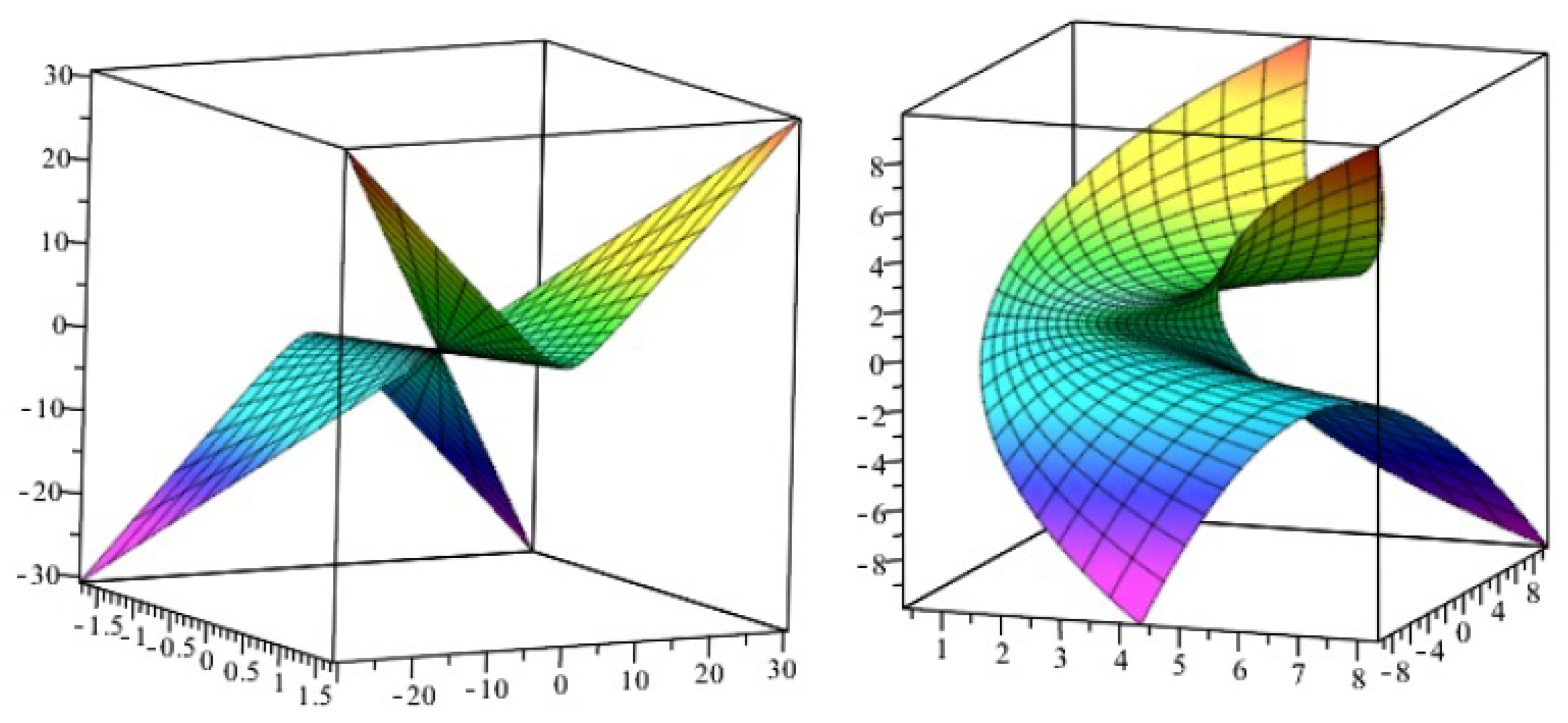
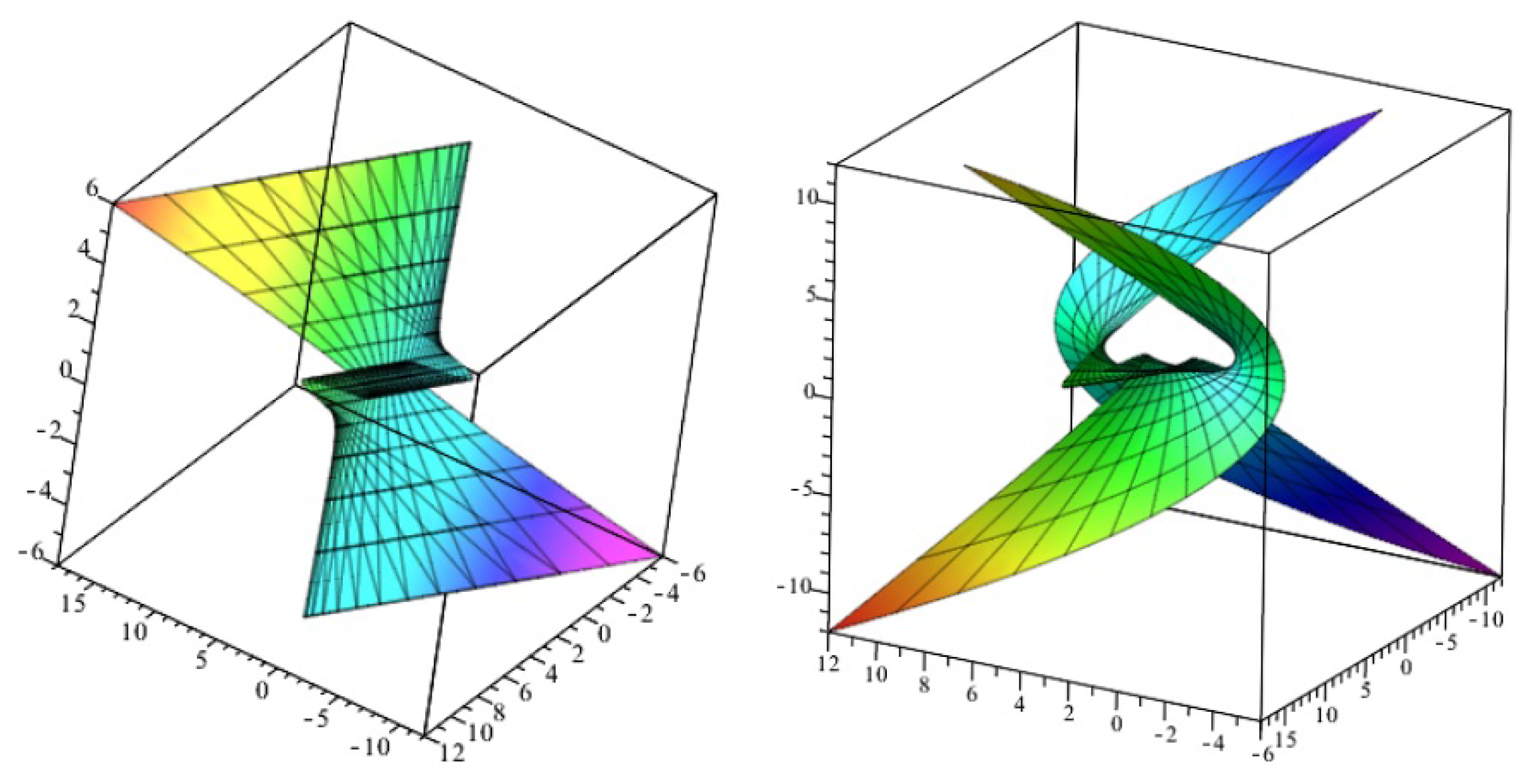
where $u,a,b\in \mathbb{R}\backslash \left\{0\right\}$ and $0\le v,w\le 2\pi .$ See Figure 1 and Figure 2 to projections of $\mathbf{H}$ with spacelike axis into three-space.

Computing the first differentials of (1), we get the first quantities as follows

$$I=\left(\begin{array}{ccc}{\phi }^{\prime }{}^2-1& a{\phi }^{\prime }& b{\phi }^{\prime }\\ a{\phi }^{\prime }& u^2{cosh}^{2}w+a^2& ab\\ b{\phi }^{\prime }& ab& u^2+b^2\end{array}\right),$$

where $\phi =\phi \left(u\right),$ ${\phi }^{\prime }=\frac{d\phi }{du}.$ Thus, we have

$$detI=u^2\left[(u^2({\phi }^{\prime }{}^2-1)-b^2){cosh}^{2}w-a^2\right].$$

With the second differentials with respect to $u,v,w,$ we obtain the second quantities as follows

$$II=\left(\begin{array}{ccc}-\frac{u^2{\phi }^{″}coshw}{\sqrt{detI}}& \frac{aucoshw}{\sqrt{detI}}& \frac{ubcoshw}{\sqrt{detI}}\\ \frac{aucoshw}{\sqrt{detI}}& \frac{u^2(u{\phi }^{\prime }coshw-bsinhw){cosh}^{2}w}{\sqrt{detI}}& \frac{a{u}^{2}sinhw}{\sqrt{detI}}\\ \frac{ubcoshw}{\sqrt{detI}}& \frac{a{u}^{2}sinhw}{\sqrt{detI}}& \frac{u^3{\phi }^{\prime }coshw}{\sqrt{detI}}\end{array}\right)$$

and

$$\begin{array}{ccc}\hfill detII& =& \frac{u^{4}coshw}{{\left(detI\right)}^{3/2}}[\left(-u^4{\phi }^{\prime }{}^2{cosh}^{4}w+b{u}^3{\phi }^{\prime }{cosh}^{3}wsinhw+a^2{u}^2{sin}^{2}w\right){\phi }^{″}\hfill \\ & & -u{cosh}^{2}w\left(a^2+b^2{cosh}^{2}w\right){\phi }^{\prime }+b^3{cosh}^{3}wsinhw-2a^{2}bcoshwsinh].\hfill \end{array}$$

Hence, the Gauss map of the helicoidal hypersurface is given by

$$e_{\mathbf{H}}=-\frac{1}{\sqrt{detI}}\left(\begin{array}{c}{u}^{2}coshw\\ u\left[(u{\phi }^{\prime }sinhw-bcoshw)\right]coshw\\ u\left[(u{\phi }^{\prime }coshw-bsinhw)sinhvcoshw-acoshv\right]\\ u\left[(u{\phi }^{\prime }coshw-bsinhw)coshvcoshw-asinhv\right]\end{array}\right).$$

Finally, we calculate the Gaussian curvature and the mean curvature of the helicoidal hypersurface with spacelike axis and state the results in the following propostion:

Proposition 1.

For a helicodal hypersurface with spacelike axis in ${\mathbb{E}}_1^4$ the Gaussian and mean curvatures, respectively, are as follows

$$K=\frac{{\lambda }_1{\phi }^{\prime }{}^2{\phi }^{″}+{\lambda }_2{\phi }^{\prime }{\phi }^{″}+{\lambda }_3{\phi }^{″}+{\lambda }_4{\phi }^{\prime }+{\lambda }_5}{{\left(detI\right)}^{5/2}},H=\frac{{\zeta }_1{\phi }^{″}+{\zeta }_2{\phi }^{\prime }{}^3+{\zeta }_3{\phi }^{\prime }{}^2+{\zeta }_4{\phi }^{\prime }+{\zeta }_5}{3{\left(detI\right)}^{3/2}},$$

where

• ${\lambda }_1=-u^8{cosh}^{5}w,$
• ${\lambda }_2=b{u}^{7}sinhw{cosh}^{4}w,$
• ${\lambda }_3=a^2{u}^{6}coshw{sinh}^{2}w,$
• ${\lambda }_4=u^5(b^2{cosh}^{2}w+a^2){cosh}^{3}w,$
• ${\lambda }_5=-b{u}^4(b^2{cosh}^{2}w+2a^2)sinhw{cosh}^{2}w,$
• ${\zeta }_1=u^4\left[\left(u^2+b^2\right){cosh}^{2}w+a^2\right]coshw,$
• ${\zeta }_2=-2u^5{cosh}^{3}w,$
• ${\zeta }_3=b{u}^4{cosh}^{2}wsinhw,$
• ${\zeta }_4=u^3\left[3a^2+\left(3b^2+2u^2\right){cosh}^{2}w\right]coshw,$
• ${\zeta }_5=b{u}^2\left[\left(u^2+b^2\right){cosh}^{2}w-2a^2\right]sinhw.$

Corollary 1.

When $\phi =c=const.,$ we get

$$K=\frac{-b{u}^4(b^2{cosh}^{2}w+2a^2)sinhw{cosh}^{2}w,}{{\left[u^2(b^2+u^2){cos}^{2}w+a^2\right]}^{5/2}},H=\frac{b{u}^2\left[\left(u^2+b^2\right){cosh}^{2}w-2a^2\right]sinhw}{3{\left[u^2\left((b^2+u^2){cos}^{2}w+a^2\right)\right]}^{3/2}}.$$

Corollary 2.

When $\phi =c=const.$ and $b=0,$ we have $K=0,$ $H=0.$

4. Helicoidal Hypersurfaces with Timelike Axis

Taking ${\ell }_2$ is the line spanned by the timelike vector ${\left(0,0,0,1\right)}^t$, the orthogonal matrix is given by

$${\mathbf{A}}_2(v,w)=\left(\begin{array}{cccc}cosvcosw& -sinv& -cosvsinw& 0\\ sinvcosw& cosv& -sinvsinw& 0\\ sinw& 0& cosw& 0\\ 0& 0& 0& 1\end{array}\right),$$

where $v,w\in \mathbb{R}.$ The matrix ${\mathbf{A}}_2$ can be found by

$$det{\mathbf{A}}_2=1,{\mathbf{A}}_2.{\ell }_2={\ell }_2,{\mathbf{A}}_2^t\epsilon {\mathbf{A}}_2=\epsilon ,$$

where $\epsilon =diag(1,1,1,-1).$ When the axis of rotation is ${\ell }_2$, there is an Minkowskian transformation by which the axis is ${\ell }_2$ transformed to the $x_4$-axis of ${\mathbb{E}}_1^4$. Parametrization of the profile curve is given by

$$\gamma \left(u\right)=\left(u,0,0,\phi \left(u\right)\right),$$

where $\phi \left(u\right)$ is a differentiable function for all $u\in I$. Thus, the helicoidal hypersurface which is spanned by the vector $\left(0,0,0,1\right)$ with pitches $a,b\in \mathbb{R}\backslash \left\{0\right\}$, is as follows

$$\mathbf{H}(u,v,w)={\mathbf{A}}_2(v,w)\gamma {\left(u\right)}^t+(av+bw){(0,0,0,1)}^t$$

in ${\mathbb{E}}_1^4,$ where $u\in I,$ $v,w\in \left[0,2\pi \right].$ If $w=0,$ we get helicoidal surface with timelike axis as in the three dimensional Minkowski space ${\mathbb{E}}_1^3$.

When $a=b=0$, the surface is just a rotational hypersurface with timelike axis as follows

$$\mathbf{R}(u,v,w)=\left(ucosvcosw,usinvcosw,usinw,\phi \left(u\right)\right).$$

Now, we obtain the mean curvature and the Gaussian curvature of a helicoidal hypersurface with timelike axis

$$\mathbf{H}(u,v,w)=\left(\begin{array}{c}ucosvcosw\\ usinvcosw\\ usinw\\ \phi \left(u\right)+av+bw\end{array}\right),$$

(2)

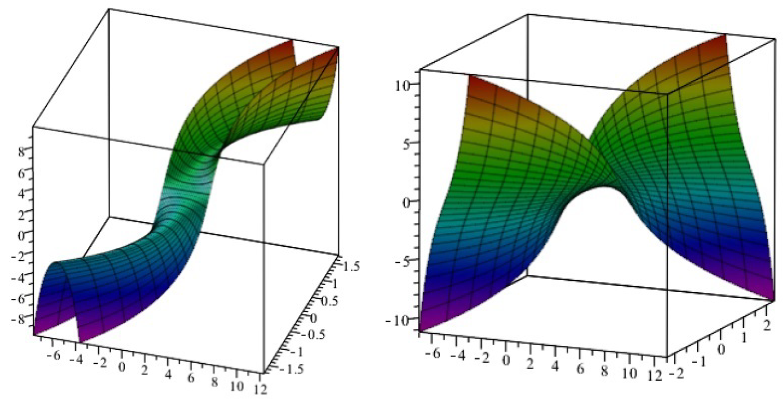
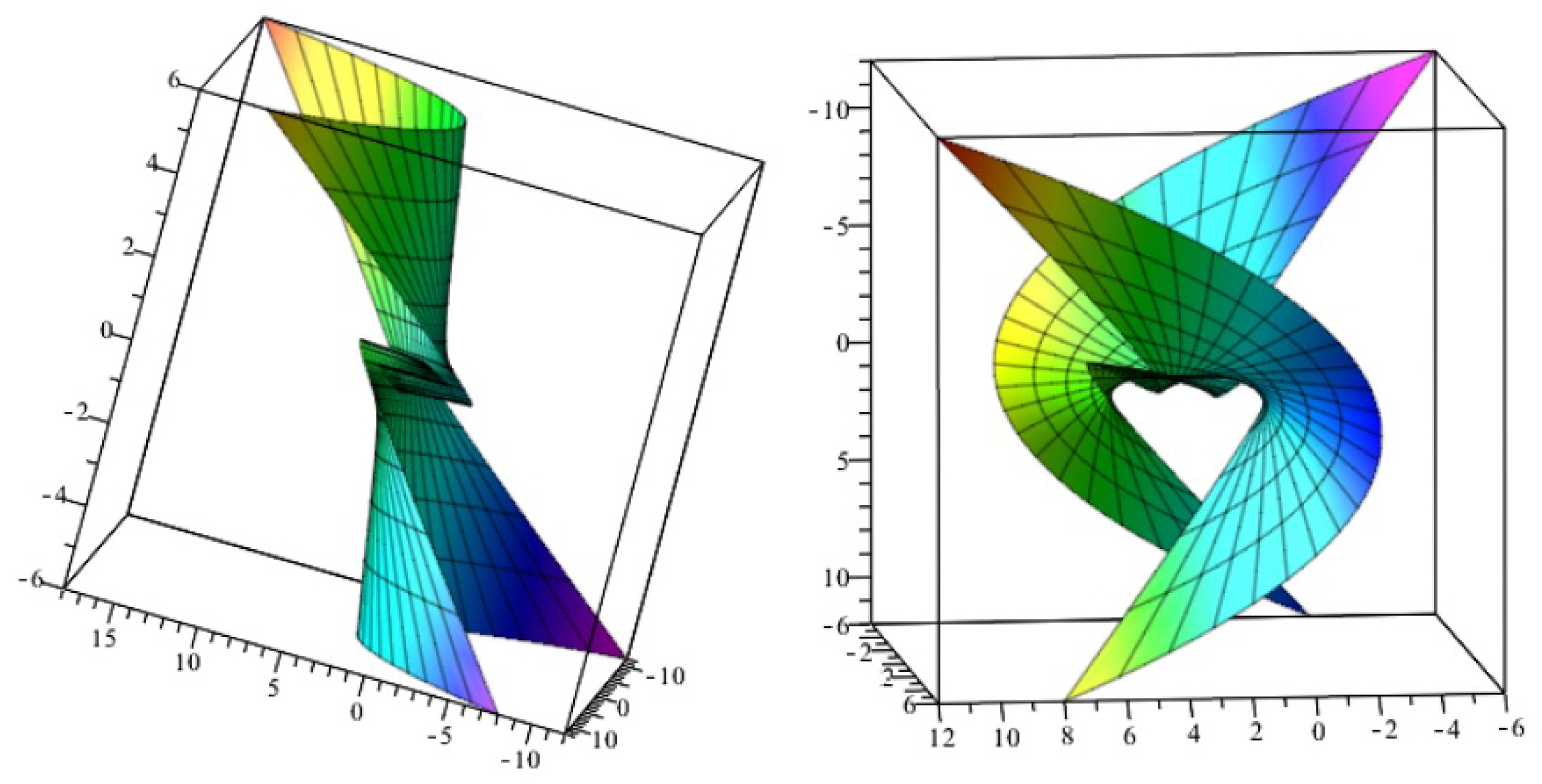
where $u,a,b\in \mathbb{R}\backslash \left\{0\right\}$ and $0\le v,w\le 2\pi .$ See Figure 3 and Figure 4 to projections of $\mathbf{H}$ with timelike axis into three-space.

Computing the first differentials of (2), we find the first quantities

$$I=\left(\begin{array}{ccc}1-{\phi }^{\prime }{}^2& -a{\phi }^{\prime }& -b{\phi }^{\prime }\\ -a{\phi }^{\prime }& u^2{cos}^{2}w-a^2& -ab\\ -b{\phi }^{\prime }& -ab& u^2-b^2\end{array}\right),$$

where $\phi =\phi \left(u\right),$ ${\phi }^{\prime }=\frac{d\phi }{du}.$ Then, we get

$$detI=u^2\left[(u^2(1-{\phi }^{\prime }{}^2)-b^2){cos}^{2}w-a^2\right].$$

With the second differentials with respect to $u,v,w,$ we have the second quantities

$$II=\left(\begin{array}{ccc}-\frac{u^2{\phi }^{″}cosw}{\sqrt{\left|detI\right|}}& \frac{aucosw}{\sqrt{\left|detI\right|}}& \frac{ubcosw}{\sqrt{\left|detI\right|}}\\ \frac{aucosw}{\sqrt{\left|detI\right|}}& -\frac{u^2(u{\phi }^{\prime }cosw-bsinw){cos}^{2}w}{\sqrt{\left|detI\right|}}& -\frac{a{u}^{2}sinw}{\sqrt{\left|detI\right|}}\\ \frac{ubcosw}{\sqrt{\left|detI\right|}}& -\frac{a{u}^{2}sinw}{\sqrt{\left|detI\right|}}& -\frac{u^3{\phi }^{\prime }cosw}{\sqrt{\left|detI\right|}}\end{array}\right)$$

and

$$\begin{array}{ccc}\hfill detII& =& \frac{u^{4}cosw}{{\left|detI\right|}^{3/2}}[-u^4{\phi }^{\prime }{}^2{\phi }^{″}{cos}^{4}w+b{u}^3{\phi }^{\prime }{\phi }^{″}{cos}^{3}wsinw+a^2{u}^2{\phi }^{″}{sin}^{2}w\hfill \\ & & +u{cos}^{2}w\left(-a^2+b^2{cos}^{2}w\right){\phi }^{\prime }+b^3{cos}^{3}wsinw-2a^{2}bcoswsinw].\hfill \end{array}$$

Then, the Gauss map of the helicoidal hypersurface is given by

$$e_{\mathbf{H}}=\frac{1}{\sqrt{detI}}\left(\begin{array}{c}u\left[(u{\phi }^{\prime }cosw-bsinw)cosvcosw-asinv\right]\\ u\left[(u{\phi }^{\prime }cosw-bsinw)sinvcosw+acosv\right]\\ u\left[(u{\phi }^{\prime }sinw+bcosw)\right]cosw\\ u^{2}cosw\end{array}\right).$$

Finally, we calculate the Gaussian curvature and the mean curvature of the helicoidal hypersurface with timelike axis and state the results in the following propostion.

Proposition 2.

For a helicodal hypersurface with timelike axis in ${\mathbb{E}}_1^4$ the Gaussian and mean curvatures, respectively, are as follows

$$K=\frac{{\beta }_1{\phi }^{\prime }{}^2{\phi }^{″}+{\beta }_2{\phi }^{\prime }{\phi }^{″}+{\beta }_3{\phi }^{″}+{\beta }_4{\phi }^{\prime }+{\beta }_5}{{\left|detI\right|}^{5/2}},H=\frac{{\eta }_1{\phi }^{″}+{\eta }_2{\phi }^{\prime }{}^3+{\eta }_3{\phi }^{\prime }{}^2+{\eta }_4{\phi }^{\prime }+{\eta }_5}{3{\left|detI\right|}^{3/2}},$$

where

• ${\beta }_1=-u^8{cos}^{5}w,$
• ${\beta }_2=b{u}^{7}sinw{cos}^{4}w,$
• ${\beta }_3=a^2{u}^{6}cosw{sin}^{2}w,$
• ${\beta }_4=u^5(b^2{cos}^{2}w+a^2){cos}^{3}w,$
• ${\beta }_5=-b{u}^4(b^2{cos}^{2}w+2a^2)sinw{cos}^{2}w,$
• ${\eta }_1=u^4\left(\left(u^2+b^2\right){cos}^{2}w+a^2\right)cosw,$
• ${\eta }_2=2u^5{cos}^{3}w,$
• ${\eta }_3=b{u}^4{cos}^{2}wsinw,$
• ${\eta }_4=-u^3\left(3a^2+\left(3b^2+2u^2\right){cos}^{2}w\right)cosw,$
• ${\eta }_5=-b{u}^2\left(\left(u^2-b^2\right){cos}^{2}w-2a^2\right)sinw.$

Corollary 3.

When $\phi =c=const.,$ then we have

$$K=\frac{-b{u}^4(b^2{cos}^{2}w+2a^2)sinw{cos}^{2}w}{{\left|u^2\left[(u^2-b^2){cos}^{2}w-a^2\right]\right|}^{5/2}},H=\frac{-b{u}^2\left(\left(u^2-b^2\right){cos}^{2}w-2a^2\right)sinw}{3{\left|u^2\left[(u^2-b^2){cos}^{2}w-a^2\right]\right|}^{3/2}}.$$

Corollary 4.

When $\phi =c=const.$ and $b=0,$ we have the same situation of Corollary 2, i.e., K and H vanish.

5. Helicoidal Hypersurfaces with Lightlike Axis

Considering ${\ell }_3$ is the line spanned by the lightlike vector ${\left(0,0,1,1\right)}^t$, the orthogonal matrix is given by

$${\mathbf{A}}_3(v,w)=\left(\begin{array}{cccc}1& 0& -v& v\\ 0& 1& -w& w\\ v& w& 1-\frac{1}{2}\left(v^2+w^2\right)& \frac{1}{2}\left(v^2+w^2\right)\\ v& w& -\frac{1}{2}\left(v^2+w^2\right)& 1+\frac{1}{2}\left(v^2+w^2\right)\end{array}\right),$$

where $v,w\in \mathbb{R}.$ The matrix ${\mathbf{A}}_3$ can be found by

$$det{\mathbf{A}}_3=1,{\mathbf{A}}_3.{\ell }_3={\ell }_3,{\mathbf{A}}_3^t\epsilon {\mathbf{A}}_3=\epsilon ,$$

where $\epsilon =diag(1,1,1,-1).$ When the axis of rotation is ${\ell }_3$, there is an Minkowskian transformation by which the axis is ${\ell }_3$ transformed to the $x_3{x}_4$-axis of ${\mathbb{E}}_1^4$. Parametrization of the profile curve is given by

$$\gamma \left(u\right)=\left(0,0,\phi \left(u\right),u\right),$$

where $\phi \left(u\right):I\subset \mathbb{R}⟶\mathbb{R}$ is a differentiable function for all $u\in I$. So, the helicoidal hypersurface which is spanned by the lightlike vector $\left(0,0,1,1\right)$ with pitches $a,b\in \mathbb{R}\backslash \left\{0\right\}$, is as follows:

$$\mathbf{H}(u,v,w)={\mathbf{A}}_3(v,w)\gamma {\left(u\right)}^t+(av+bw){(0,0,1,1)}^t$$

in ${\mathbb{E}}_1^4,$ where $u\in I,$ $v,w\in \mathbb{R}.$ When $w=0,$ we get helicoidal surface with lightlike axis as in the three dimensional Minkowski space ${\mathbb{E}}_1^3$.

When $a=b=0$, the surface is just a rotational hypersurface with lightlike axis as follows

$$\mathbf{R}(u,v,w)=\left(\begin{array}{c}uv-\phi \left(u\right)v,\\ uw-\phi \left(u\right)w\\ \frac{1}{2}u\left(v^2+w^2\right)+\left[1-\frac{1}{2}\left(v^2+w^2\right)\right]\phi \left(u\right)\\ u\left[1+\frac{1}{2}\left(v^2+w^2\right)\right]+\left[-\frac{1}{2}\left(v^2+w^2\right)\right]\phi \left(u\right)\end{array}\right).$$

Next, we obtain the curvatures of a helicoidal hypersurface with lightlike axis

$$\mathbf{H}(u,v,w)=\left(\begin{array}{c}uv-\phi \left(u\right)v\\ uw-\phi \left(u\right)w\\ \frac{1}{2}u\left(v^2+w^2\right)+\left[1-\frac{1}{2}\left(v^2+w^2\right)\right]\phi \left(u\right)+av+bw\\ u\left[1+\frac{1}{2}\left(v^2+w^2\right)\right]+\left[-\frac{1}{2}\left(v^2+w^2\right)\right]\phi \left(u\right)+av+bw\end{array}\right),$$

(3)

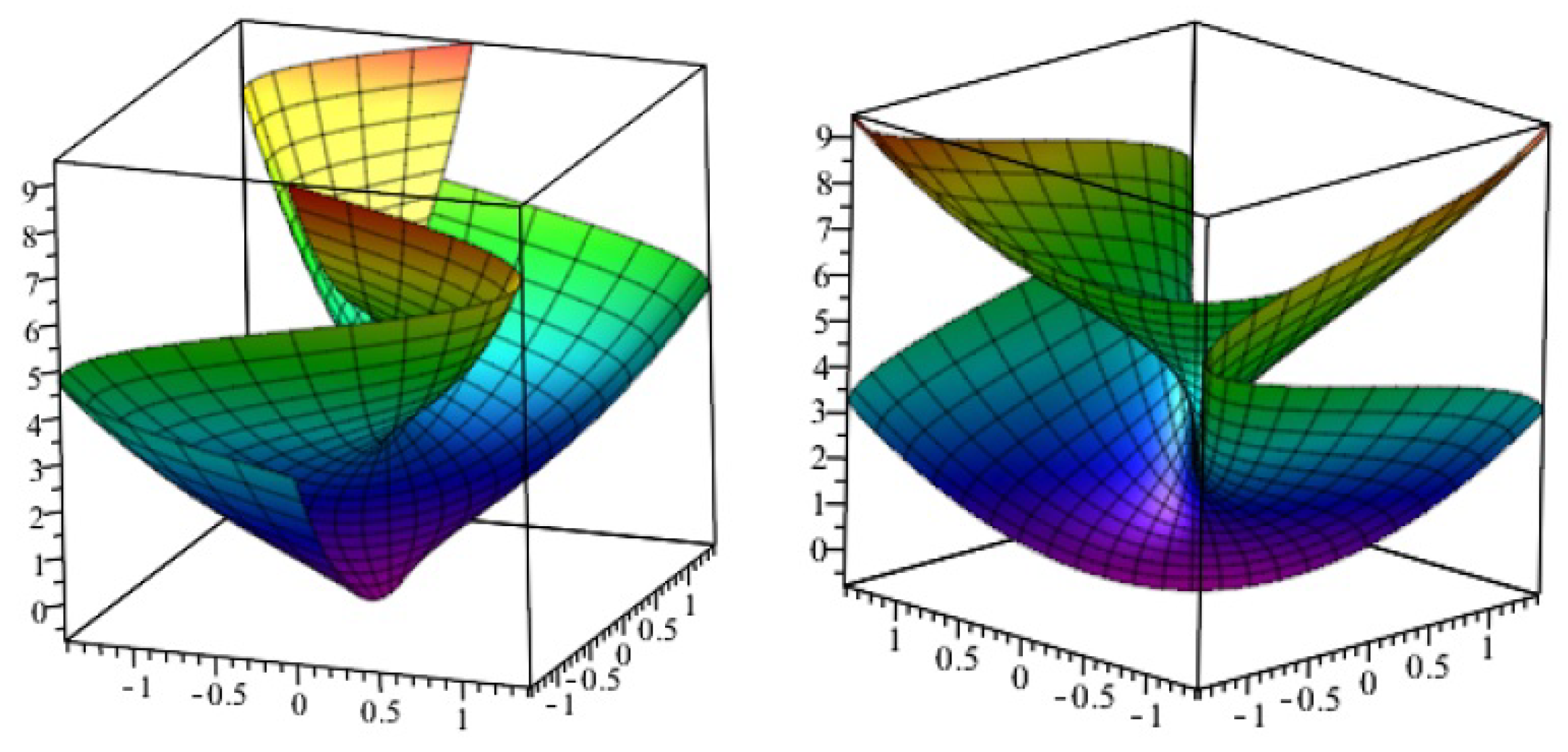
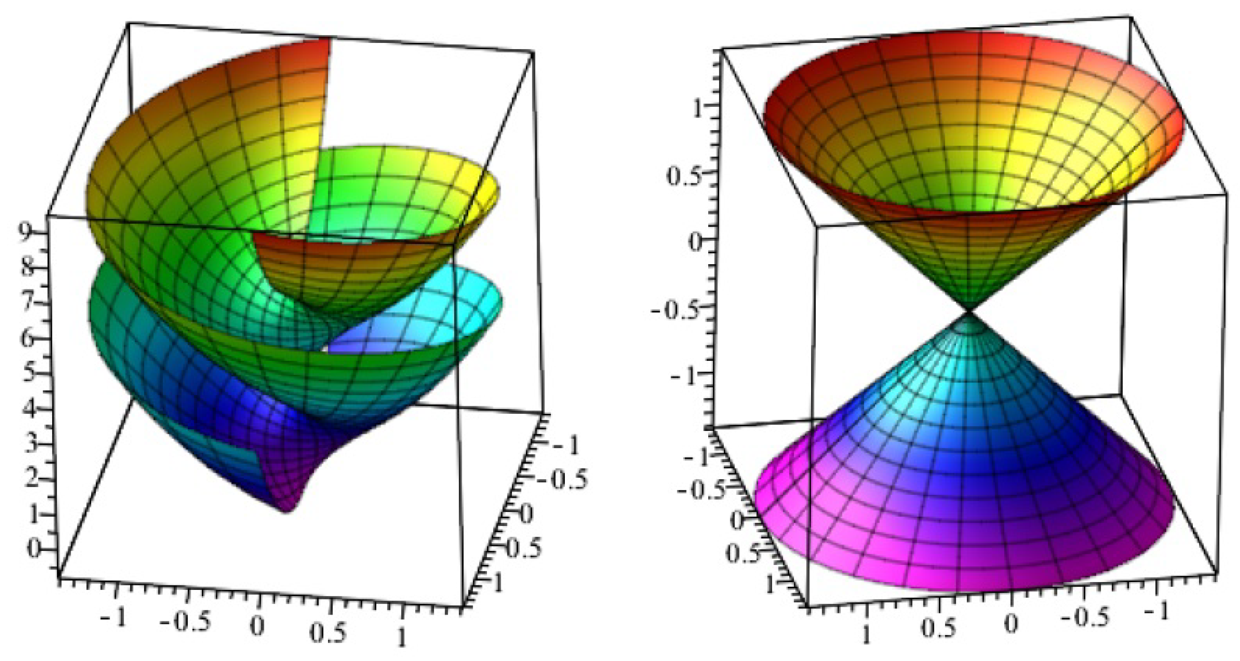
where $u,a,b\in \mathbb{R}\backslash \left\{0\right\}$ and $v,w\in \mathbb{R}.$ See Figure 5 and Figure 6 to projections of $\mathbf{H}$ with lightlike axis into three-space.

Calculating the first differentials of (3), we obtain the first quantities

$$I=\left(\begin{array}{ccc}{\phi }^{\prime }{}^2-1& a\left({\phi }^{\prime }-1\right)& b\left({\phi }^{\prime }-1\right)\\ a\left({\phi }^{\prime }-1\right)& {\left(\phi -u\right)}^2& 0\\ b\left({\phi }^{\prime }-1\right)& 0& {\left(\phi -u\right)}^2\end{array}\right),$$

where $\phi =\phi \left(u\right),$ ${\phi }^{\prime }=\frac{d\phi }{du}.$ Then, we have

$$detI={\left(\phi -u\right)}^2\left[{\left(\phi -u\right)}^2\left({\phi }^{\prime }{}^2-1\right)-\left(a^2+b^2\right){\left({\phi }^{\prime }-1\right)}^2\right].$$

With the second differentials with respect to $u,v,w,$ we have the second quantities

$$II=\left(\begin{array}{ccc}-\frac{{\left(\phi -u\right)}^2{\phi }^{″}}{\sqrt{detI}}& \frac{a{\left({\phi }^{\prime }-1\right)}^2\left(u-\phi \right)}{\sqrt{detI}}& \frac{b{\left({\phi }^{\prime }-1\right)}^2\left(u-\phi \right)}{\sqrt{detI}}\\ \frac{a{\left({\phi }^{\prime }-1\right)}^2\left(u-\phi \right)}{\sqrt{detI}}& -\frac{{\left(\phi -u\right)}^3\left({\phi }^{\prime }-1\right)}{\sqrt{detI}}& 0\\ \frac{b{\left({\phi }^{\prime }-1\right)}^2\left(u-\phi \right)}{\sqrt{detI}}& 0& -\frac{{\left(\phi -u\right)}^3\left({\phi }^{\prime }-1\right)}{\sqrt{detI}}\end{array}\right).$$

Hence, the Gauss map of the hypersurface is given by

$$e_{\mathbf{H}}=\frac{h}{2\sqrt{detI}}\left(\begin{array}{c}\delta \left(hv-a\right)\\ \delta \left(hw-b\right)\\ \left(v^2+w^2\right)h\delta +2h-2\delta \left(av+bw\right)\\ \left(v^2+w^2\right)h\delta +2h{\phi }^{\prime }-2\delta \left(av+bw\right)\end{array}\right),$$

where $\delta ={\phi }^{\prime }-1,$ $h=\phi -u.$ Finally, we calculate the Gaussian curvature and the mean curvature of the helicoidal hypersurface with lightlike axis, respectively, as follows

$$K=\frac{h^5{\delta }^2\left[\left(u^3-{\phi }^3\right){\phi }^{″}+3uh\phi {\phi }^{″}+\left(a^2+b^2\right){\delta }^3\right]}{{\left(detI\right)}^2{\left|detI\right|}^{1/2}},$$

(4)

and

$$H=\frac{h^5{\phi }^{″}+2h^2\left[2h^2\delta \left({\phi }^{\prime }{}^2-1\right)-3\left(a^2+b^2\right){\delta }^3\right]}{3detI{\left|detI\right|}^{1/2}}.$$

(5)

We assume that $detI>0.$ Therefore, the problem now is reduced to finding the solution of this differential equation in $\phi =\phi \left(u\right)$, where the function $K=K\left(u\right)$ is the known smooth function given.

Next, we will examine Equation (4). Let $h\left(u\right)=\phi \left(u\right)-u$, then $h^{\prime }\left(u\right)={\phi }^{\prime }\left(u\right)-1$ and $h^{″}\left(u\right)={\phi }^{″}\left(u\right).$ Hence, (4) reduces to

$$K\left(u\right)=\frac{h^{\prime }{}^2\left(c^2{h}^{\prime }{}^3-h^3{h}^{″}\right)}{{\left[h^2{h}^{\prime }\left(h^{\prime }+2\right)-c^2{h}^{\prime }{}^2\right]}^{5/2}},$$

(6)

where $c^2=a^2+b^2.$

In order to get an idea for these hypersurfaces, we study $K=0$, $K<0,$ $K>0,K=const.$ and $H=0$ for some special functional forms of the curvatures.

Case 1. $K\left(u\right)=0.$ Equation (6) takes the form

$$h^{\prime }{}^2\left(c^2{h}^{\prime }{}^3-h^3{h}^{″}\right)=0.$$

(7)

Suppose that

$$h^{\prime }=t\Rightarrow h^{″}=t\frac{dt}{dh}.$$

(8)

Then Equation (7) reduces to

$$c^2{t}^5-h^3{t}^3\frac{dt}{dh}=0.$$

The solution of this equation is given by

$$t=\frac{2h^2}{2c_1{h}^2-c^2},c_1\in \mathbb{R}.$$

From Equation (8) we get

$$\frac{dh}{du}=\frac{2h^2}{2c_1{h}^2-c^2}.$$

Hence, we have

$$\frac{c^2}{2h}+c_{1}h=u+c_2,c_2\in \mathbb{R}.$$

If $c_1=0$, then $h\left(u\right)=\frac{c^2}{2\left(u+c_2\right)},$ and find

$$\phi \left(u\right)=\frac{c^2}{2\left(u+c_2\right)}+u,c_2\in \mathbb{R}.$$

Moreover, we define following one-parameter family of curves

$$\gamma \left(u\right)\equiv \gamma \left(K\left(u\right),c;c_2\right)=\left(0,0,\frac{c^2}{2\left(u+c_2\right)}+u,u\right).$$

(9)

Therefore, the equation of these helicoidal hypersurfaces $\mathbf{H}(u,v,w)$ is given by

$$\left(\begin{array}{c}uv-\left(\frac{c^2}{2\left(u+c_2\right)}+u\right)v\\ uw-\left(\frac{c^2}{2\left(u+c_2\right)}+u\right)w\\ \frac{1}{2}u\left(v^2+w^2\right)+\left[1-\frac{1}{2}\left(v^2+w^2\right)\right]\left(\frac{c^2}{2\left(u+c_2\right)}+u\right)+av+bw\\ u\left[1+\frac{1}{2}\left(v^2+w^2\right)\right]+\left[-\frac{1}{2}\left(v^2+w^2\right)\right]\left(\frac{c^2}{2\left(u+c_2\right)}+u\right)+av+bw\end{array}\right),$$

(10)

where $c=\sqrt{a^2+b^2}.$

If $c_1\ne 0$ then $h\left(u\right)=\frac{u+c_2\pm \sqrt{{\left(u+c_2\right)}^2-2c_1{c}^2}}{2c_1},$ and we obtain

$$\phi \left(u\right)=\frac{u+c_2\pm \sqrt{{\left(u+c_2\right)}^2-2c_1{c}^2}}{2c_1}+u,c_2\in \mathbb{R}.$$

Then, we define following two-parameter family of curves

$$\gamma \left(u\right)\equiv \gamma \left(K\left(u\right),c;c_1,c_2\right)=\left(0,0,\frac{u+c_2\pm \sqrt{{\left(u+c_2\right)}^2-2c_1{c}^2}}{2c_1}+u,u\right).$$

(11)

Hence, the equation of these helicoidal hypersurfaces is given by

$$\left(\begin{array}{c}uv-\left(\frac{u+c_2\pm \sqrt{{\left(u+c_2\right)}^2-2c_1{c}^2}}{2c_1}+u\right)v\\ uw-\left(\frac{u+c_2\pm \sqrt{{\left(u+c_2\right)}^2-2c_1{c}^2}}{2c_1}+u\right)w\\ \frac{1}{2}u\left(v^2+w^2\right)+\left[1-\frac{1}{2}\left(v^2+w^2\right)\right]\left(\frac{u+c_2\pm \sqrt{{\left(u+c_2\right)}^2-2c_1{c}^2}}{2c_1}+u\right)+av+bw\\ u\left[1+\frac{1}{2}\left(v^2+w^2\right)\right]+\left[-\frac{1}{2}\left(v^2+w^2\right)\right]\left(\frac{u+c_2\pm \sqrt{{\left(u+c_2\right)}^2-2c_1{c}^2}}{2c_1}+u\right)+av+bw\end{array}\right).$$

(12)

Finally, we observe that given the function $K\left(u\right)=0$, we can determine a one or two-parameter family of curves given by (9) or (11), respectively, and define the corresponding Equations (10) or (12) of the helicoidal hypersurfaces with lightlike axis immersed in ${\mathbb{E}}_1^4.$

Case 2(a). When $c_1<0$ and $detI>0,$ Equation (6) takes the form

$$K\left(u\right)=\frac{h^{\prime }{}^2\left(c^2{h}^{\prime }{}^3-h^3{h}^{″}\right)}{{\left|h^2{h}^{\prime }\left(h^{\prime }+2\right)-c^2{h}^{\prime }{}^2\right|}^{5/2}}=\frac{c_1^5{c}^2}{{\left|c_1\left(c_1+2\right){\left(c_{1}u+c_2\right)}^2-c^2{c}_1^2\right|}^{5/2}}<0$$

(13)

which is satisfied by the function $h\left(u\right)=c_{1}u+c_2$ and therefore $\phi =(c_1+1)u+c_2$, where $u\ne -\frac{1}{c_1^2\left(c_1+2\right)}\left(c_1^2{c}_2\pm c\sqrt{c_1^3\left(c_1+2\right)}+2c_1{c}_2\right),$ $c_1\in \mathbb{R}\backslash \left\{-2,0\right\}.$ So, given the function $K=K\left(u\right)$ by (13) following the same process there exists a family of helicoidal hypersurfaces $\mathbf{H}(u,v,w)$ immersed in ${\mathbb{E}}_1^4,$ the equation of which is

$$\left(\begin{array}{c}uv-((c_1+1)u+c_2)v\\ uw-((c_1+1)u+c_2)w\\ \frac{1}{2}u\left(v^2+w^2\right)+\left[1-\frac{1}{2}\left(v^2+w^2\right)\right]((c_1+1)u+c_2)+av+bw\\ u\left[1+\frac{1}{2}\left(v^2+w^2\right)\right]+\left[-\frac{1}{2}\left(v^2+w^2\right)\right]((c_1+1)u+c_2)+av+bw\end{array}\right).$$

Similarly, when $c_1>0$ and $detI>0,$ Equation (6) reduces to $K\left(u\right)>0.$

Case 2(b). Equation (6) takes the form

$$K\left(u\right)=\frac{{\left(2c_{1}u+c_2\right)}^2\left(c^2{\left(2c_{1}u+c_2\right)}^3-2c_1{\left(c_1{u}^2+c_{2}u+c_3\right)}^3\right)}{{\left[{\left(c_1{u}^2+c_{2}u+c_3\right)}^2\left(2c_{1}u+c_2\right)\left(\left(2c_{1}u+c_2\right)+2\right)-c^2{\left(2c_{1}u+c_2\right)}^2\right]}^{5/2}},$$

(14)

which is satisfied by the function $h\left(u\right)=c_1{u}^2+c_{2}u+c_3$ and therefore $\phi =c_1{u}^2+(c_2+1)u+c_3$, where $c_i\in \mathbb{R}.$ So, given the function $K=K\left(u\right)$ by (14) following the same process there exists a family of helicoidal hypersurfaces $\mathbf{H}(u,v,w)$ immersed in ${\mathbb{E}}_1^4,$ the equation of which is

$$\left(\begin{array}{c}uv-(c_1{u}^2+(c_2+1)u+c_3)v\\ uw-(c_1{u}^2+(c_2+1)u+c_3)w\\ \frac{1}{2}u\left(v^2+w^2\right)+\left[1-\frac{1}{2}\left(v^2+w^2\right)\right](c_1{u}^2+(c_2+1)u+c_3)+av+bw\\ u\left[1+\frac{1}{2}\left(v^2+w^2\right)\right]+\left[-\frac{1}{2}\left(v^2+w^2\right)\right](c_1{u}^2+(c_2+1)u+c_3)+av+bw\end{array}\right).$$

Case 2(c). We consider $K=d=const.$, $d\in \mathbb{R}\backslash \left\{0\right\}.$ Then we get

$$d^2{\left[h^2{h}^{\prime }\left(h^{\prime }+2\right)-c^2{h}^{\prime }{}^2\right]}^5-h^{\prime }{}^4{\left(c^2{h}^{\prime }{}^3-h^3{h}^{″}\right)}^2=0.$$

Using the substitution $h^{\prime }=t,$ the equation reduces to

$$d^2{t}^5{\left[\left(h^2-c^2\right)t+2h^2\right]}^5-t^6{\left(c^2{t}^2-h^3\frac{dt}{dh}\right)}^2=0.$$

We could not compute this equation using analytical methods. It is the future problem for us.

Case 3. Now, we think $\phi =\phi \left(u\right)$ such that $h^{\prime }\left(u\right)={\phi }^{\prime }\left(u\right)-1\ne 0$ for every $u\in \mathbb{R}\backslash \left\{0\right\}.$ So, we can consider the inverse function $u=u\left(h\right)$. Then, Equation (6) can be written as

$$K\left(u\left(h\right)\right)=\frac{h^{\prime }{}^2\left(c^2{h}^{\prime }{}^3-h^3{h}^{″}\right)}{{\left[h^2{h}^{\prime }\left(h^{\prime }+2\right)-c^2{h}^{\prime }{}^2\right]}^{5/2}}.$$

Taking $h^{\prime }=t,$ it takes the form

$$t^6{\left(c^2{t}^2-h^3\frac{dt}{dh}\right)}^2-K^2{t}^5{\left[\left(h^2-c^2\right)t+2h^2\right]}^5=0.$$

If we do not know some particular solution, we can not get its general solution.

Case 4. The mean curvature of the helicoidal hypersurface given by (3) in the Minkowski space ${\mathbb{E}}_1^4$ is given by (5). The problem now is to find the solution of this equation in $\phi =\phi \left(u\right)$, where the function $H=H\left(u\right)$ is the known smooth function given. Since we may give the solution of the equation

$$h^5{\phi }^{″}+2h^2\left[2h^2\delta \left({\phi }^{\prime }{}^2-1\right)-3\left(a^2+b^2\right){\delta }^3\right]=0,$$

we can find the helicoidal minimal hypersurfaces. Taking $h\left(u\right)=\phi \left(u\right)-u,$ $\delta =h^{\prime }\left(u\right)={\phi }^{\prime }\left(u\right)-1,$ $h^{″}\left(u\right)={\phi }^{″}\left(u\right)$ then this equation takes the form

$$h^5{h}^{″}+\left(4h^4-6c^2{h}^2\right)h^{\prime }{}^3+8h^4{h}^{\prime }{}^2=0,$$

where $c^2=a^2+b^2.$ So, using $h^{\prime }\left(u\right)=t\left(u\right)$ it reduces to

$$t^{-2}\frac{dt}{dh}+\frac{8}{ht}+\frac{4h^4-6c^2{h}^2}{h^5}=0.$$

Setting $\varphi =1/t,$ we get

$$\frac{d\varphi }{dh}-\frac{8}{h}\varphi -\frac{4h^4-6c^2{h}^2}{h^5}=0.$$

Solution of above equation is

$$\varphi =\frac{1}{t}=\frac{40c_1{h}^{10}-5h^5+24c^2}{40h^2},c_1\in \mathbb{R}.$$

Therefore, we see that $h=h\left(u\right)$ (resp. $\phi =\phi \left(u\right)$) satisfy the following equations:

$$\begin{array}{c}12800c_1^2{h}^{20}-2200c_1{h}^{15}-12800c_1{h}^{12}+\left(5760c_1{c}^2+75\right)h^{10}\\ +1600h^7-120c^2{h}^5-6400h^4+1920c^2{h}^2-1152c^4=0,\end{array}$$

and

$$\begin{array}{c}12800c_1^2{\left(\phi -u\right)}^{20}-2200c_1{\left(\phi -u\right)}^{15}-12800c_1{\left(\phi -u\right)}^{12}\\ +\left(5760c_1{c}^2+75\right){\left(\phi -u\right)}^{10}+1600{\left(\phi -u\right)}^7-120c^2{\left(\phi -u\right)}^5\\ -6400{\left(\phi -u\right)}^4+1920c^2{\left(\phi -u\right)}^2-1152c^4=0.\end{array}$$

Hence, for every function $\phi =\phi \left(u\right)$ which satisfies the last equation, there exists a helicoidal minimal hypersurface with lightlike axis in ${\mathbb{E}}_1^4$ whose parametric representation is given by (3).

We were not able to find the solution of Equation (5) by using analytical methods, so, it is for us, an open problem. Nevertheless, one could consider special values for the function $H=H\left(u\right)$ as we did earlier for the function $K=K\left(u\right)$, and then give solutions of the corresponding equations. For example, if

$$H\left(u\right)=\frac{4e^{4u}+9e^{3u}-6c^2{e}^{2u}}{3{\left[e^{4u}+2e^{3u}-c^2{e}^{2u}\right]}^{3/2}},$$

where $u\ne ln\left(-1+\sqrt{1+c^2}\right),$ then (5) reduces to

$$\frac{4e^{4u}+9e^{3u}-6c^2{e}^{2u}}{{\left[e^{4u}+2e^{3u}-c^2{e}^{2u}\right]}^{3/2}}=\frac{h^5{h}^{″}+\left(4h^4-6c^2{h}^2\right)h^{\prime }{}^3+8h^4{h}^{\prime }{}^2}{h^3{\left[h^2{h}^{\prime }\left(h^{\prime }+2\right)-c^2{h}^{\prime }{}^2\right]}^{3/2}}.$$

(15)

This equation is satisfied by the function $h\left(u\right)=e^u$ and then $\phi \left(u\right)=e^u+u.$ Here, when $H=0$ then $4e^{4u}+9e^{3u}-6c^2{e}^{2u}=0.$ So, we have $u=ln\left(\frac{-9\pm \sqrt{3\left(32c^2+27\right)}}{8}\right).$

Given the function $H=H\left(u\right)$ by (15), there exists a helicoidal hypersurface with lightlike axis immersed in ${\mathbb{E}}_1^4$ the equation of which is given by

$$\mathbf{H}(u,v,w)=\left(\begin{array}{c}uv-\left(e^u+u\right)v\\ uw-\left(e^u+u\right)w\\ \frac{1}{2}u\left(v^2+w^2\right)+\left[1-\frac{1}{2}\left(v^2+w^2\right)\right]\left(e^u+u\right)+av+bw\\ u\left[1+\frac{1}{2}\left(v^2+w^2\right)\right]+\left[-\frac{1}{2}\left(v^2+w^2\right)\right]\left(e^u+u\right)+av+bw\end{array}\right).$$

Finally, we give the following theorem:

Theorem 1.

Let $\gamma \left(u\right)=\left(0,0,\phi \left(u\right),u\right)$, $u\in I\subset \mathbb{R}$ be a profile curve of the helicoidal hypersurface $\mathbf{M}$ immersed in ${\mathbb{E}}_1^4$ given by (3). Then the Gaussian and the mean curvature at the point $\left(0,0,\phi \left(u\right),u\right)$ are functions of the same variable u, i.e., $K=K\left(u\right),$ $H=H\left(u\right)$. Moreover, given constants $a,b\in I\subset {\mathbb{R}}^{+}$, $c_1,c_2\in \mathbb{R}$ and a smooth function $K=K\left(u\right)$ (resp. $H=H\left(u\right)$), $u\in I$ we define the family of curves $\gamma \left(u\right)\equiv \gamma (K\left(u\right),c;c_1,c_2)$ (resp. $\gamma \left(u\right)\equiv \gamma (H\left(u\right),c;c_1,c_2)$).

6. Helicoidal Hypersurface with Timelike Axis satisfying ${\Delta }^I\mathbf{H}=A\mathbf{H}$ in ${\mathbb{E}}_1^4$

The Gauss map of the helicoidal hypersurface with timelike axis (2) is clearly given by

$$e=\frac{1}{W}\left(\begin{array}{c}(u{\phi }^{\prime }cosw-bsinw)cosvcosw-asinv\\ (u{\phi }^{\prime }cosw-bsinw)sinvcosw+acosv\\ (u{\phi }^{\prime }sinw+bcosw)cosw\\ ucosw\end{array}\right),$$

where $W=\sqrt{(u^2(1-{\phi }^{\prime }{}^2)-b^2){cos}^{2}w-a^2}.$ We use

$$-3He=A\mathbf{H},$$

and we get

$$\left(\begin{array}{c}\left[\Omega (u{\phi }^{\prime }cosw)-u{a}_{11}\right]cosvcosw-\left(a\Omega +ucosw{a}_{12}\right)sinv-\left(b\Omega cosvcosw+u{a}_{13}\right)sinw\\ \left[\Omega (u{\phi }^{\prime }cosw)-u{a}_{22}\right]sinvcosw+\left(a\Omega -ucosw{a}_{21}\right)cosv-\left(b\Omega sinvcosw+u{a}_{23}\right)sinw\\ \left(u{\phi }^{\prime }\Omega cosw-u{a}_{33}\right)sinw+\left(b\Omega cosw-usinv{a}_{32}-ucosv{a}_{31}\right)cosw\\ u\Omega cosw\end{array}\right)$$

$$=\left(\begin{array}{c}\left(\phi +av+bw\right)a_{14}\\ \left(\phi +av+bw\right)a_{24}\\ \left(\phi +av+bw\right)a_{34}\\ ucosvcosw{a}_{41}+usinvcosw{a}_{42}+u{a}_{43}sinw+\left(\phi +av+bw\right)a_{44}\end{array}\right),$$

where A is a $4\times 4$ matrix, and $\mathrm{\Omega }\left(u,w\right)=\frac{3H}{W}.$ The equation ${\Delta }^I\mathbf{H}=A\mathbf{H}$ by means of the first quantities $I,$ and ${\Delta }^I\mathbf{H}=-3He$ leads to the following system of ODEs:

$$\begin{array}{cc}& \left(\Omega u{\phi }^{\prime }cosw-u{a}_{11}\right)cosvcosw-\left(a\Omega +ucosw{a}_{12}\right)sinv-\left(b\Omega cosvcosw+u{a}_{13}\right)sinw\hfill \\ =& \left(\phi +av+bw\right)a_{14},\hfill \\ & \left(\Omega u{\phi }^{\prime }cosw-u{a}_{21}\right)sinvcosw+\left(a\Omega -ucosw{a}_{22}\right)cosv-\left(b\Omega sinvcosw+u{a}_{23}\right)sinw\hfill \\ =& \left(\phi +av+bw\right)a_{24},\hfill \\ & \left(\Omega u{\phi }^{\prime }cosw-u{a}_{33}\right)sinw+\left(b\Omega cosw-usinv{a}_{32}-ucosv{a}_{31}\right)cosw\hfill \\ =& \left(\phi +av+bw\right)a_{34},\hfill \\ & u\Omega cosw\hfill \\ =& ucosvcosw{a}_{41}+usinvcosw{a}_{42}+usinw{a}_{43}+\left(\phi +av+bw\right)a_{44}.\hfill \end{array}$$

Differentiating ODE’s twice with respect to $v,$ we have

$$a_{14}=a_{24}=a_{34}=a_{44}=0,\Omega \left(u,w\right)=0.$$

(16)

From (16), we get

$$\begin{array}{cc}-a_{11}ucosvcosw-a_{12}ucoswsinv-a_{13}usinw\hfill & =0,\hfill \\ -a_{21}usinvcosw-a_{22}ucoswcosv-a_{23}usinw\hfill & =0,\hfill \\ -a_{31}ucosvcosw-a_{32}usinv-a_{33}usinw\hfill & =0,\hfill \\ a_{41}ucosvcosw+a_{42}usinvcosw+a_{43}usinw\hfill & =0.\hfill \end{array}$$

cosine and sine are linearly independent functions of v, then we see $a_{ij}=0$. Since $\Omega \left(u,w\right)=\frac{3H}{W}$, we have $H=0$. Consequently, $\mathbf{H}$ is a minimal hypersurface with timelike axis.

Therefore, we have following theorem:

Theorem 2.

Let timelike $\mathbf{H}$: $M_1^3$⟶${\mathbb{E}}_1^4$ be an isometric immersion given by (2). Then ${\Delta }^I\mathbf{H}=A\mathbf{H},$ where A is a $4\times 4$ matrix iff the mean curvature of $\mathbf{H}$ vanishes.

7. Open Problems

An umbilical point is an significant geometric qualification, related to lines of curvature. Since a line of curvature will end at such points, it is a singularity of a line of curvature. It can partially be because there is an powerful criterion for a smooth (hyper)surface defined by a formula, for both parametric or implicit (hyper)surfaces:

Lemma 1.

A point is an umbilical point iff $H^2-K=0$ at this point.

Finding the umbilic points, we calculate $det(\mathbf{S}-\lambda I_3)=0$, and also we use the equation in Lemma 1 for three hypersurfaces in this paper. Hence, we have following problems:

Problem 1.

Solve following differential equation for helicoidal hypersurface with spacelike axis (1):

$$u{\left[\left(b^2+u^2\left(1-{\phi }^{\prime }{}^2\right)\right){cosh}^{2}w+a^2\right]}^{1/2}+\frac{9}{2}{u}^2\left[\left(b^2+u^2\left(1-{\phi }^{\prime }{}^2\right)\right){cosh}^{2}w+a^2\right]coshw$$

$$.{\left(\begin{array}{c}-\frac{1}{2}{u}^4{\phi }^{\prime }{}^2{\phi }^{″}{cosh}^{4}w-\frac{1}{2}u{cosh}^{2}w\left(-b{u}^2{\phi }^{″}coshwsinhw+b^2{cosh}^{2}w+a^2\right){\phi }^{\prime }\\ +\left[\frac{1}{2}{a}^2{u}^2{\phi }^{″}sinhw+\left(\frac{1}{2}{b}^2{cosh}^{2}w+a^2\right)bcoshw\right]\end{array}\right)}^{2}sinhw$$

$$.{\left(\begin{array}{c}{u}^3{\phi }^{\prime }{}^3{cosh}^{3}w-\frac{1}{2}b{u}^2{\phi }^{\prime }{}^2{cosh}^{2}wsinhw-\frac{3}{2}u{\phi }^{\prime }\left[\left(b^2+\frac{2}{3}{u}^2\right){\left(a^2+coshw\right)}^2\right]coshw\\ -\frac{1}{2}{u}^{2}coshw\left[\left(b^2+u^2\right){cosh}^{2}w+a^2\right]{\phi }^{″}+\left[a^2+\frac{1}{2}\left(b^2+u^2\right){cosh}^{2}w\right]bsinhw\end{array}\right)}^2=0.$$

Problem 2.

Solve following differential equation for helicoidal hypersurface with timelike axis (2):

$$u{\left[\left(u^2{\phi }^{\prime }{}^2+b^2-u^2\right){cos}^{2}w+a^2\right]}^{1/2}-\frac{9}{2}\left[\left(u^2\left({\phi }^{\prime }{}^2-1\right)+b^2\right){cos}^{2}w+a^2\right]$$

$$.{\left(\begin{array}{c}-u^3{\phi }^{\prime }{}^3{cos}^{3}w+\frac{1}{2}b{u}^2{\phi }^{\prime }{}^2{cos}^{2}wsinw-\frac{3}{2}\left(\left(b^2-\frac{2}{3}{u}^2\right){cos}^{2}w+a^2\right)u{\phi }^{\prime }cosw\\ -\frac{1}{2}\left[\left(b^2-u^2\right){cos}^{2}w+a^2\right]u^2{\phi }^{″}cosw+\left[\frac{1}{2}\left(b^2-u^2\right){cos}^{2}w+a^2\right]bsinw\end{array}\right)}^2$$

$$.{\left(\begin{array}{c}\frac{1}{2}{u}^4{\phi }^{\prime }{}^2{\phi }^{″}{cos}^{4}w-\frac{1}{2}u{cos}^{2}w\left(u^{2}b{\phi }^{″}coswsinw+b^2{cos}^{2}w+a^2\right){\phi }^{\prime }\\ +\left[-\frac{1}{2}{a}^2{u}^2{\phi }^{″}sinw+\left(\frac{1}{2}{b}^2{cos}^{2}w+a^2\right)bsinwcosw\right]\end{array}\right)}^2{u}^{2}cosw=0.$$

Problem 3.

Solve following differential equation for helicoidal hypersurface with lightlike axis (3):

$$\begin{array}{c}{\left(\begin{array}{c}\left[a^2+b^2-\frac{2}{3}{\left(u-\phi \right)}^2\right]{\phi }^{\prime }{}^3+\left[-3\left(a^2+b^2\right)+\frac{2}{3}{\left(u-\phi \right)}^2\right]{\phi }^{\prime }{}^2\\ +\left[3\left(a^2+b^2\right)+\frac{2}{3}{\left(u-\phi \right)}^2\right]{\phi }^{\prime }-\left[\left(a^2+b^2\right)+\frac{2}{3}{\left(u-\phi \right)}^2\right]+\frac{1}{3}{\left(u-\phi \right)}^3{\phi }^{″}\end{array}\right)}^2\hfill \\ .{\left({\phi }^{\prime }-1\right)}^{1/2}{\left[\left({\left(u-\phi \right)}^2-\left(a^2+b^2\right)\right){\phi }^{\prime }+{\left(u-\phi \right)}^2+a^2+b^2\right]}^{3/2}\hfill \\ -{\left[\left(a^2+b^2-{\left(u-\phi \right)}^2\right){\phi }^{\prime }-\left(a^2+b^2\right)-{\left(u-\phi \right)}^2\right]}^2\hfill \\ .{\left({\phi }^{\prime }-1\right)}^3\left[\left(a^2-b^2\right){\left({\phi }^{\prime }-1\right)}^3+{\left(u-\phi \right)}^3{\phi }^{″}\right]=0.\hfill \end{array}$$

All $\phi$ solutions in the problems will give umbilic points of the hypersurfaces.