Solving Higher-Order Boundary and Initial Value Problems via Chebyshev–Spectral Method: Application in Elastic Foundation

Abstract

In this work, we introduce an efficient scheme for the numerical solution of some Boundary and Initial Value Problems (BVPs-IVPs). By using an operational matrix, which was obtained from the first kind of Chebyshev polynomials, we construct the algebraic equivalent representation of the problem. We will show that this representation of BVPs and IVPs can be represented by a sparse matrix with sufficient precision. Sparse matrices that store data containing a large number of zero-valued elements have several advantages, such as saving a significant amount of memory and speeding up the processing of that data. In addition, we provide the convergence analysis and the error estimation of the suggested scheme. Finally, some numerical results are utilized to demonstrate the validity and applicability of the proposed technique, and also the presented algorithm is applied to solve an engineering problem which is used in a beam on elastic foundation.

1. Introduction

Initial value problems, boundary value problems, and other related problems have many applications in physics, chemistry, and different research areas (see, e.g., in [1,2,3,4,5,6,7,8,9,10,11] and the references given therein). Most higher order of these types of equations and problems do not have exact analytical solutions, thus approximation techniques must be applied.

In this work, we shall discuss the following BVPs.

$$\sum _{i=0}^n{a}_i{D}^{i}u\left(x\right)=R\left(x\right),x\in [-1,1],$$

(1)

with

$$\beta {}_{k0}u(-1)+\sum _{j=1}^{n-1}\beta {}_{kj}{u}^{\left(j\right)}\left(1\right)=l_k,(k=0,1,2,\dots ,n-1),$$

(2)

and also the following IVPs,

$$\sum _{i=0}^n{a}_i{D}^{i}u\left(x\right)=R\left(x\right),x\in [0,1],$$

(3)

with

$$\sum _{j=0}^{n-1}\beta {}_{kj}{u}^{\left(j\right)}\left(0\right)=l_k,(k=0,1,2,\dots ,n-1),$$

(4)

where $a_i,\beta {}_{kj}\in \mathbb{R}$ are constants, $(i=0,1,\dots ,n)$, $(j,k=0,1,\dots ,n-1)$, and $R\left(x\right)$ and $u\left(x\right)$ are given and unknown functions, respectively.

Among numerical approaches, spectral methods are very successful and powerful tools for the numerical solution of differential and integral equations involving derivatives of integer and non-integer order. Effective properties that have encouraged many experts in numerical analysis to use spectral methods for different kinds of mathematical problems are spectral accuracy and the ease of applying these methods. One of the most important advantages of these methods is their high accuracy, the so-called convergence of “infinite order”. Therefore, when the exact solution is infinitely differentiable, the numerical approximation converges faster than $M^{-n}$, where M is the order of approximation and $n>0$ is constant [12,13].

Pseudospectral, Galerkin, and Tau methods are several kinds of spectral methods which can be obtained from a weighted residual method [12]. The Tau method, which can be explained as a special case of spectral methods, was invented by Lanczos [14]. It has become increasingly popular with applications in many disciplines such as porous media, viscoelasticity, electrochemistry, and other problems where high accuracy is desired. Further detailed information of this procedure can be found in [15,16,17].

In the literature, there are several approaches to obtain numerical methods to solve boundary value problems and other related problems such as Chebyshev-type, Runge–Kutta type, Wavelet–Galerkin method, and Shannon approximation [5,6,18,19,20,21,22,23]. Wolf [24] has been concerned with the numerical solution of non-singular integral and integro-differential equations by iteration with Chebyshev series. In [25], a Chebyshev series were used for nonlinear differential equations. Various works, such as the works in [26,27], introduced and discussed a Chebyshev technique for solving nonlinear optimal control problems. Mezzadri et al. [28] have been concerned with nonlinear programming methods for the solution of optimal control problems via a Chebyshev technique.

The proposed approach in this work is referred to as operational in the sense that it makes it possible to transform a given differential equation into an algebraic equation. An efficient algorithm of the Tau approximation based on Chebyshev polynomials is presented to numerically solve the boundary and initial value problems. One of the main advantages of this methodology is that the matrices generated of BVPs and IVPs are sparse. The proposed procedure can be very attractive to users who are concerned with memory conservation, much less computational cost and much more computational speed (see Remark 2). Furthermore, the simplicity of the scheme and low algorithm run time are among its other advantages. Ultimately, to demonstrate the validity and applicability of the method, an engineering problem of the fourth-order ODE which is arising in elastic foundation is solved.

The organization of this paper is as follows. In Section 2, we present the basic properties of Chebyshev polynomials. Converting boundary value problem (1) and initial value problem (3) to a matrix form based on the new proposed algorithm is shown and the convergence analysis for the first kind of Chebyshev expansion is given in Section 3. The last part of this work is concerned with four numerical examples to illustrate the method.

2. Some Preliminaries

Now, we remind some basic properties and essentials of Chebyshev polynomials, which are applied further in this work [1].

Definition 1.

The first kind of Chebyshev polynomials of order n is described as

$$T_n\left(x\right)=cos\left[nco{s}^{-1}x\right],x\in [-1,1],n=0,1,2,\dots .$$

(5)

Furthermore, due to (5), we can write

$$T_n(cos\theta )=cos\left(n\theta \right),\theta \in [0,\pi ],n=0,1,2,\dots .$$

Theorem 1.

The Chebyshev polynomials $T_n\left(x\right)$ satisfy the following relation,

$$T_{n+1}\left(x\right)=2x{T}_n\left(x\right)-T_{n-1}\left(x\right),n=1,2,\dots .$$

(6)

Remark 1.

Using simple computation the following relations with derivatives of Chebyshev polynomials can be obtained,

$$\left\{\begin{array}{c}{T}_0\left(x\right)=T_1^{{}^{\prime }}\left(x\right),\hfill \\ T_1\left(x\right)=\frac{1}{4}{T}_2^{{}^{\prime }}\left(x\right),\hfill \\ T_n\left(x\right)=[\frac{T_{n+1}^{{}^{\prime }}\left(x\right)}{2(n+1)}-\frac{T_{n-1}^{{}^{\prime }}\left(x\right)}{2(n-1)}],\hfill & n\ge 2.\hfill \end{array}\right.$$

(7)

Proposition 1.

Chebyshev polynomials are orthogonal functions:

$${\int }_{-1}^1{T}_n\left(x\right)T_m\left(x\right){(1-x^2)}^{-1/2}dx=\frac{\pi }{2}{c}_n{\delta }_{nm},$$

(8)

where ${(1-x^2)}^{-1/2}$ is weighting function and

$$c_n=\left\{\begin{array}{cc}2\hfill & n=0,\hfill \\ 1\hfill & n>0,\hfill \end{array}\right.and{\delta }_{nm}=\left\{\begin{array}{cc}0\hfill & n\ne m,\hfill \\ 1\hfill & n=m.\hfill \end{array}\right.$$

(9)

The Chebyshev polynomials $T_n\left(x\right)$ are defined on the interval $[-1,1]$. In order to use these polynomials on the interval $x\in [a,b]$, we introduce $x=\frac{b-a}{2}t+\frac{b+a}{2}$.

3. Outline of the Method for Boundary and Initial Value Problems

Here, Chebyshev–Tau method is expressed to solve boundary value problem (1) and initial value problem (3). The first part is concerned with the matrix structure produced by proposed method, the convergence, and the error analysis for the mentioned polynomials. The second part will be discussed with the numerical solvability of the system of algebraic equations arising in the presented method.

3.1. Operational Matrix of Derivative

Let functions $u\left(x\right)$ and $Du\left(x\right)$ be expanded by the Chebyshev polynomials in $[-1,1]$ as

$$u\left(x\right)=\sum _{n=0}^{\infty }{\nu }_n{T}_n\left(x\right)={\mathbf{T}}_x{\mathbf{V}}^T,$$

(10)

$$Du\left(x\right)=\sum _{n=0}^{\infty }{\omega }_{1,n}{T}_n\left(x\right)={\mathbf{T}}_x{\mathbf{W}}_1^T,$$

(11)

where $\mathbf{V}=({\nu }_0,{\nu }_1,{\nu }_2,\dots )$, ${\mathbf{W}}_1=({\omega }_{1,0},{\omega }_{1,1},{\omega }_{1,2},\dots )$ and $T_x=(T_0\left(x\right),T_1\left(x\right),T_2\left(x\right),\dots )$. Moreover, for any integrable function $u\left(x\right)$ on $[-1,1]$, we define ${\nu }_n$ as follows,

$${\nu }_n=<u\left(x\right),T_n\left(x\right)>=\frac{2}{\pi c_n}{\int }_{-1}^{1}u\left(x\right)T_n\left(x\right)\omega \left(x\right)dx.$$

Taking the derivative of (10), we have

$$Du\left(x\right)=\sum _{n=1}^{\infty }{\nu }_n{T}_n^{{}^{\prime }}\left(x\right).$$

(12)

Due to (11) and (12), we obtain

$$\sum _{n=1}^{\infty }{\nu }_n{T}_n^{{}^{\prime }}\left(x\right)={\omega }_{1,0}{T}_0\left(x\right)+{\omega }_{1,1}{T}_1\left(x\right)+\sum _{n=2}^{\infty }{\omega }_{1,n}{T}_n\left(x\right),$$

by using Equation (7), we can rewrite the last equation as follows,

$$\Rightarrow {\nu }_1{T}_1^{{}^{\prime }}\left(x\right)+{\nu }_2{T}_2^{{}^{\prime }}\left(x\right)+{\nu }_3{T}_3^{{}^{\prime }}\left(x\right)+\dots ={\omega }_{1,0}{T}_1^{{}^{\prime }}\left(x\right)+\frac{{\omega }_{1,1}}{4}{T}_2^{{}^{\prime }}\left(x\right)+\sum _{n=2}^{\infty }\frac{{\omega }_{1,n}}{2}[\frac{T_{n+1}^{{}^{\prime }}\left(x\right)}{n+1}-\frac{T_{n-1}^{{}^{\prime }}\left(x\right)}{n-1}],$$

then we conclude that

$$\left\{\begin{array}{c}{\nu }_{{}_1}=\frac{1}{2}[2{\omega }_{{}_{1,0}}-{\omega }_{{}_{1,2}}],\hfill \\ {\nu }_{{}_2}=\frac{1}{4}[{\omega }_{1,1}-{\omega }_{{}_{1,3}}],\hfill \\ {\nu }_{{}_3}=\frac{1}{6}[{\omega }_{1,2}-{\omega }_{{}_{1,4}}],\hfill \\ ⋮\hfill \\ {\nu }_{{}_{N-2}}=\frac{1}{2(N-2)}[{\omega }_{{}_{1,N-3}}-{\omega }_{{}_{1,N-1}}],\hfill \\ ⋮\hfill \end{array}\right.$$

(13)

or equivalently

$$\left\{\begin{array}{c}{\omega }_{{}_{1,0}}={\nu }_{{}_1}+3{\nu }_{{}_3}+5{\nu }_{{}_5}+\dots +\frac{{\tau }_{0,N-1}}{2}{\nu }_{{}_{N-1}}+\frac{{\tau }_{0,N}}{2}{\nu }_{{}_N}+\dots ,\hfill \\ {\omega }_{{}_{1,i}}=\sum _{n=i+1}^{\infty }{\nu }_n{\tau }_{i,n},i\ge 1,\hfill \end{array}\right.$$

(14)

where

$${\tau }_{i,n}=\left\{\begin{array}{c}0,i+neven,\hfill \\ 2n,o.w.\hfill \end{array}\right.$$

Let us introduce matrix $\mathbf{E}$ as a coefficient of matrix $\mathbf{V}$, then from (14) we have ${\mathbf{W}}_1^T=\mathbf{E}{\mathbf{V}}^T$. The upper triangular matrix $\mathbf{E}$, via easy calculations, is as follows,

$$\mathbf{E}=\left[\begin{array}{ccccccccc}0& 1& 0& 3& 0& 5& 0& 7& \cdots \\ 0& 0& 4& 0& 8& 0& 12& 0& \cdots \\ 0& 0& 0& 6& 0& 10& 0& 14& \cdots \\ ⋮& ⋮& ⋮& ⋮& ⋮& ⋮& ⋮& ⋮& ⋮\end{array}\right].$$

Theorem 2.

Let $D^{k}u\left(x\right)={\sum }_{n=0}^{\infty }{\omega }_{k,n}{T}_n\left(x\right)={\mathbf{T}}_x{\mathbf{W}}_k^T$ be a Chebyshev polynomial with

$${\mathbf{W}}_k=[{\omega }_{k,0},{\omega }_{k,1},{\omega }_{k,2},\cdots ],{\mathbf{T}}_x=[T_0\left(x\right),T_1\left(x\right),T_2\left(x\right),\cdots ],\mathbf{V}=[{\nu }_0,{\nu }_1,{\nu }_2,\dots ],$$

then for any $k\in \mathbb{N}$, we obtain

$$D^{k}u\left(x\right)={\mathbf{T}}_x{\mathbf{E}}^k{\mathbf{V}}^T.$$

Proof. 

As we pointed out previously, Equation (14) can be written to the following matrix structure,

$${\mathbf{W}}_1={\left(\mathbf{E}{\mathbf{V}}^T\right)}^T=\mathbf{V}{\mathbf{E}}^T.$$

(15)

Furthermore, due to Equation (11), we have

$$Du\left(x\right)={\mathbf{T}}_x\mathbf{E}{\mathbf{V}}^T.$$

From Equation (7), we can write

$$T_n^{{}^{\prime }}\left(x\right)=\frac{1}{2}[\frac{T_{n+1}^{{}^{″}}\left(x\right)}{n+1}-\frac{T_{n-1}^{{}^{″}}\left(x\right)}{n-1}].$$

Given the assumption, it follows that

$$D^{2}u\left(x\right)=\sum _{n=0}^{\infty }{\omega }_{2,n}{T}_n\left(x\right)={\mathbf{T}}_x{\mathbf{W}}_2^T.$$

(16)

Using the process of obtaining Equation (15), we conclude

$${\mathbf{W}}_2^T=\mathbf{E}{\mathbf{W}}_1^T.$$

(17)

Due to (15) and the last equation, we get ${\mathbf{W}}_2^T={\mathbf{E}}^2{\mathbf{V}}^T$. Therefore, by repeating this scheme, it follows that ${\mathbf{W}}_k^T={\mathbf{E}}^k{\mathbf{V}}^T$, and we can write

$$D^{k}u\left(x\right)={\mathbf{T}}_x{\mathbf{E}}^k{\mathbf{V}}^T.$$

□

The following theorem is concerned with the convergence and the error analysis for the Chebyshev expansion.

Theorem 3.

Suppose $u\left(x\right)$ is a function that satisfies ${\int }_{-1}^1{\left|u^{\left(2\right)}\left(x\right)\right|}^{2}dx<\infty$ and $|u^{\left(2\right)}\left(x\right)|\le K$ for some constant K. Then, we have

u(x) can be expanded as ${\sum }_{n=0}^{\infty }{\nu }_n{T}_n\left(x\right)$ and the series converges to $u\left(x\right)$ uniformly, in other words

$$u\left(x\right)=\sum _{n=0}^{\infty }{\nu }_n{T}_n\left(x\right),$$

where ${\nu }_n=<u\left(x\right),T_n\left(x\right)>$.

Moreover, for an error estimation the following inequality holds,

$$\mathbf{e}\le {\left(2K^2\pi \sum _{n=N+1}^{\infty }{\displaystyle \frac{1}{{(n-1)}^4}}\right)}^{{\displaystyle \frac{1}{2}}},$$

where $\mathbf{e}={\int }_{-1}^1{|u\left(x\right)-{\sum }_{n=0}^N{\nu }_n{T}_n\left(x\right)|}^2\omega \left(x\right)dx.$

Proof. 

By showing the absolute convergence of the series ${\sum }_{n=0}^{\infty }\left|{\nu }_n\right|$, it can be concluded that the series ${\sum }_{n=0}^{\infty }{\nu }_n{T}_n\left(x\right)$ converges to $u\left(x\right)$ uniformly. According to definition of ${\nu }_n$ we have

$${\nu }_n=<u\left(x\right),T_n\left(x\right)>=\frac{2}{\pi c_n}{\int }_{-1}^{1}u\left(x\right)T_n\left(x\right)\omega \left(x\right)dx,$$

substituting $\omega \left(x\right)={(1-x^2)}^{-1/2}$ and $x=cos\theta$ yields

$${\nu }_n=\frac{2}{\pi c_n}{\int }_0^{\pi }u(cos\theta )T_n(cos\theta ){(1-cos{\theta }^2)}^{-1/2}sin\theta d\theta$$

$$=\frac{2}{\pi c_n}{\int }_0^{\pi }u(cos\theta )cosn\theta d\theta .$$

Using the integration, we have:

$${\nu }_n=\frac{2}{\pi c_{n}n}{\int }_0^{\pi }{u}^{{}^{\prime }}(cos\theta )sinn\theta sin\theta d\theta$$

$$=\frac{1}{\pi c_{n}n}{\int }_0^{\pi }{u}^{{}^{\prime }}(cos\theta )[cos(n-1)\theta -cos(n+1)\theta ]d\theta$$

$$=\frac{1}{\pi c_{n}n}\left[{\int }_0^{\pi }{u}^{{}^{\prime }}(cos\theta )cos(n-1)\theta d\theta -{\int }_0^{\pi }{u}^{{}^{\prime }}(cos\theta )cos(n+1)\theta d\theta \right],$$

with integration again, ${\nu }_n$ can be obtained as

$${\nu }_n=\frac{1}{\pi c_{n}n}\left[{\displaystyle \frac{1}{n-1}}{\int }_0^{\pi }{u}^{{}^{″}}(cos\theta )sin(n-1)\theta sin\theta d\theta -{\displaystyle \frac{1}{n+1}}{\int }_0^{\pi }{u}^{{}^{″}}(cos\theta )sin(n+1)\theta sin\theta d\theta \right],$$

thus for $n>1$, (for $n=0$, $c_n=1$), we have

$$|{\nu }_n|\le \frac{1}{\pi n}{\int }_0^{\pi }|u^{{}^{″}}(cos\theta )|\left[{\displaystyle \frac{1}{n-1}}-{\displaystyle \frac{1}{n+1}}\right].$$

Furthermore, due to assumption and by simple computation, we can obtain

$$|{\nu }_n|\le {\displaystyle \frac{2K}{[n^2-1]}}\le {\displaystyle \frac{2K}{{[n-1]}^2}}.$$

Finally, the last inequality shows that the series ${\sum }_{n=0}^{\infty }\left|{\nu }_n\right|$ is absolutely convergent. Let us set

$$\mathbf{e}={\int }_{-1}^1|u\left(x\right)-\sum _{n=0}^N{\nu }_n{T}_n\left(x\right){|}^2\omega \left(x\right)dx$$

$$={\int }_{-1}^1|\sum _{n=0}^{\infty }{\nu }_n{T}_n\left(x\right)-\sum _{n=0}^N{\nu }_n{T}_n(x){|}^2\omega \left(x\right)dx$$

$$={\int }_{-1}^1|\sum _{n=N+1}^{\infty }{\nu }_n{T}_n\left(x\right){|}^2\omega \left(x\right)dx,$$

due to orthogonality of $T_n\left(x\right)$ and value of $|{\nu }_n|$, we have:

$$\mathbf{e}\le \sum _{n=N+1}^{\infty }{\left|{\nu }_n\right|}^2{\displaystyle \frac{\pi }{2}}\le 2K^2\pi \sum _{n=N+1}^{\infty }{\displaystyle \frac{1}{{[n-1]}^4}}.$$

□

3.2. Description of the Proposed Method for BVPs and IVPs

The main object of this section is applying the obtained consequence for constructing the Tau approximate solution with Chebyshev polynomials of the boundary value problem (1).

We suppose that

$$u_N\left(x\right)=\sum _{n=0}^N{\nu }_n{T}_n\left(x\right)={\mathbf{T}}_{N,x}{\mathbf{V}}_N^T,$$

(18)

$$D^n{u}_N\left(x\right)={\mathbf{T}}_{N,x}{\mathbf{E}}_N^n{\mathbf{V}}_N^T,$$

(19)

$$R\left(x\right)=\sum _{n=0}^N{b}_n{T}_n\left(x\right)={\mathbf{T}}_{N,x}{\mathbf{b}}_N^T,$$

(20)

where ${\mathbf{V}}_N=({\nu }_0,{\nu }_1,\dots ,{\nu }_N)$, ${\mathbf{T}}_{N,x}=(T_0\left(x\right),T_1\left(x\right),\dots ,T_N\left(x\right))$, ${\mathbf{b}}_N=(b_0,b_1,\dots ,b_N)$ and ${\mathbf{E}}_N$ is a finite form of $\mathbf{E}$.

Using the above relations, (1) can be written as

$$a_n{\mathbf{T}}_{N,x}{\mathbf{E}}_N^n{\mathbf{V}}_N^T+a_{n-1}{\mathbf{T}}_{N,x}{\mathbf{E}}_N^{n-1}{\mathbf{V}}_N^T+\dots +a_1{\mathbf{T}}_{N,x}{\mathbf{E}}_N{\mathbf{V}}_N^T+a_0{\mathbf{T}}_{N,x}{\mathbf{V}}_N^T={\mathbf{T}}_{N,x}{\mathbf{b}}_N^T,$$

According to the linear independence of Chebyshev polynomials, we have

$$(a_n{\mathbf{E}}_N^n+a_{n-1}{\mathbf{E}}_N^{n-1}+\dots +a_1{\mathbf{E}}_N+a_0{\mathbf{I}}_{N+1}){\mathbf{V}}_N^T={\mathbf{b}}_N^T.$$

(21)

Let us set

$$X=a_n{\mathbf{E}}_N^n+a_{n-1}{\mathbf{E}}_N^{n-1}+\dots +a_1{\mathbf{E}}_N+a_0{\mathbf{I}}_{N+1},$$

(22)

similarly, for the Equation (2) we set

$$\beta {}_{k0}\sum _{n=0}^N{\nu }_n{T}_n(-1)+\sum _{j=1}^{n-1}\beta {}_{kj}\sum _{n=0}^N{\nu }_n{T}_n^{\left(i\right)}\left(1\right)=l_k,(k=0,1,2,\dots ,n-1).$$

(23)

Due to (22) and (23), the desired matrix can be written as

$$\left[\begin{array}{c}{\mathbf{X}}_n\\ \\ \mathbf{B}\end{array}\right]\left[\begin{array}{c}{\nu }_0\\ ⋮\\ {\nu }_N\end{array}\right]=\left[\begin{array}{c}{b}_0\\ ⋮\\ b_{{}_{N-n}}\\ l_0\\ ⋮\\ l_{n-1}\end{array}\right],$$

(24)

where ${\mathbf{X}}_n$ is obtained by eliminating the last n row of matrix X and

$$\mathbf{B}=\left[\begin{array}{cccc}{\beta }_{00}& {\beta }_{01}& \dots & {\beta }_{0,n-1}\\ {\beta }_{10}& {\beta }_{11}& \dots & {\beta }_{1,n-1}\\ ⋮& ⋮& ⋮& ⋮\\ {\beta }_{n-1,0}& {\beta }_{n-1,1}& \dots & {\beta }_{n-1,n-1}\end{array}\right]\left[\begin{array}{cccc}{T}_0(-1)& T_1(-1)& \dots & T_{{}_N}(-1)\\ 0& T_1^{{}^{\prime }}\left(1\right)& \dots & T_{{}_N}^{{}^{\prime }}\left(1\right)\\ ⋮& ⋮& ⋮& ⋮\\ 0& 0& \dots & T_{{}_N}^{(n-1)}\left(1\right)\end{array}\right].$$

(25)

By solving a sparse system of above algebraic equation, we can obtained unknown $v_i$, $(i=0,1,\dots ,N)$ and finally, $u_N\left(x\right)$, the desired approximation, can be computed from the following relation,

$$u_N\left(x\right)={\mathbf{T}}_{N,x}{\mathbf{V}}_N^T.$$

The following Algorithm 1 summarizes our proposed method.

Algorithm 1: The construction of proposed method for the boundary value problems (BVPs)

Step 1. Input:       $N,n,c_{{}_{N-i}},a_i,l_j,(i=0,\dots ,n,j=0,\dots ,n-1)$;       $R\left(x\right)$; Step 2. Compute:         $b_k=\frac{2c_k}{\pi }{\int }_{-1}^{1}R\left(x\right)T_k\left(x\right){(1-x^2)}^{-\frac{1}{2}}dx$;       for $k=0,\dots ,N-n$. Step 3. Compute the matrix ${\mathbf{E}}_N$ from matrix $\mathbf{E}$. Step 4. Compute:   4.1. ${\mathbf{E}}_N^i$ from step 3, (i=2, …, n).   4.2. ${\mathbf{X}}_n$ based on $\mathbf{X}$ from (22). Step 5. Set: $$\mathbf{B}=\left[\begin{array}{cccc}{\beta }_{00}& {\beta }_{01}& \dots & {\beta }_{0,n-1}\\ {\beta }_{10}& {\beta }_{11}& \dots & {\beta }_{1,n-1}\\ ⋮& ⋮& ⋮& ⋮\\ {\beta }_{n-1,0}& {\beta }_{n-1,1}& \dots & {\beta }_{n-1,n-1}\end{array}\right]\left[\begin{array}{cccc}{T}_0(-1)& T_1(-1)& \dots & T_{{}_N}(-1)\\ 0& T_1^{{}^{\prime }}\left(1\right)& \dots & T_{{}_N}^{{}^{\prime }}\left(1\right)\\ ⋮& ⋮& ⋮& ⋮\\ 0& \dots & \dots & T_{{}_N}^{(n-1)}\left(1\right)\end{array}\right].$$ Step 6. Obtain the solution ${\mathbf{V}}_N$ from the system of (24) and set:      $u_N\left(x\right)={\mathbf{T}}_{N,x}{\mathbf{V}}_N^T$.

Construction of the Proposed Method for IVPs

Here, we consider the initial value problems (3) as

$$\sum _{i=0}^n{a}_i{D}^{i}u\left(x\right)=R\left(x\right),x\in [0,1],$$

with

$$\sum _{j=0}^{n-1}\beta {}_{kj}{u}^{\left(j\right)}\left(0\right)=l_k,(k=0,1,2,\dots ,n-1).$$

It is clear that the given scheme for BVPs (1) and Algorithm 1, with small changes, can be easily applied to these problems, thus we refrain from going into details. Only Step 5 in Algorithm 1 will be changed, and we have

$$\mathbf{B}=\left[\begin{array}{cccc}{\beta }_{00}& {\beta }_{01}& \dots & {\beta }_{0,n-1}\\ {\beta }_{10}& {\beta }_{11}& \dots & {\beta }_{1,n-1}\\ ⋮& ⋮& ⋮& ⋮\\ {\beta }_{n-1,0}& {\beta }_{n-1,1}& \dots & {\beta }_{n-1,n-1}\end{array}\right]\left[\begin{array}{cccc}{T}_0\left(0\right)& T_1\left(0\right)& \dots & T_{{}_N}\left(0\right)\\ 0& T_1^{{}^{\prime }}\left(0\right)& \dots & T_{{}_N}^{{}^{\prime }}\left(0\right)\\ ⋮& ⋮& ⋮& ⋮\\ 0& \dots & \dots & T_{{}_N}^{(n-1)}\left(0\right)\end{array}\right],$$

(26)

therefore, we can obtain ${\mathbf{V}}_N$ from the system of (24) and finally the desired solution can be achieved from $u_{N\left(x\right)}={\mathbf{T}}_{N,x}{\mathbf{V}}_N^T$.

Remark 2.

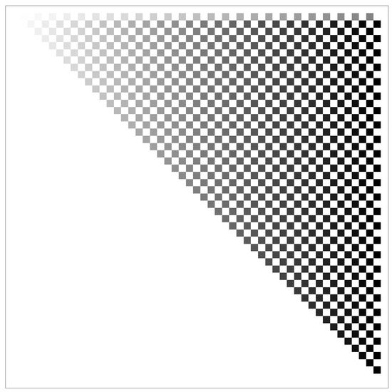
As a consequence of the described method, a significant advantage for increasing the computation speed is to the sparsity of matrices $E_N$, $E_N^2$,…,$E_N^n$. If we consider matrix $E_N$ with an odd dimension, then the number of non-zero matrix elements is ${\displaystyle \frac{N(N+2)}{4}}$. Moreover, the number of non-zero matrix elements for matrix $E_N$ with an even dimension is ${[{\displaystyle \frac{N+1}{2}}]}^2$. Furthermore, the number of non-zero matrix elements for matrix $E_N^2$ with an even and odd dimension are ${\displaystyle \frac{N^2-1}{4}}$ and ${\displaystyle \frac{N^2}{4}}$, respectively and so it goes. Figure 1, Figure 2 and Figure 3 indicate that as the derivative order rise, the sparsity of matrices and computational speed also increase.

Figure 1. The sparsity structure of $E_N$ for even value of N.

Figure 2. The sparsity structure of $E_N^2$ for even value of N.

Figure 3. The sparsity structure of $E_N^3$ for even value of N.

4. Numerical Results

In this section, the numerical results of four test problems are reported. We solve the examples using proposed Tau approximation method based on Chebyshev basis functions. In the tables presented here, the maximal differences between exact and approximation solution has been shown by “Maximal Errors”. We compare our obtained results with in the some existing numerical methods. The numerical results of the given method have been shown in Figure 4, Figure 5, Figure 6 and Figure 7.

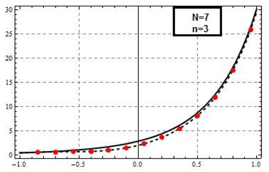
Figure 4. The Tau approximation of order 3 and $N=7$ for Example 1 using Chebyshev basis.

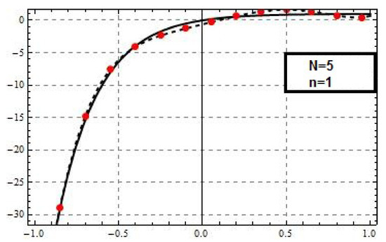
Figure 5. The Tau approximation of order 1 and $N=5$ for Example 2 using Chebyshev basis.

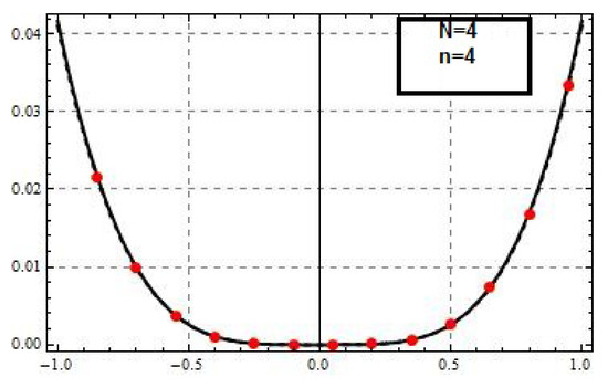
Figure 6. The Tau approximation of order 4 and $N=4$ for Example 3 using Chebyshev basis.

Figure 7. The Tau approximation of order 5 and $N=9$ for Example 4 using Chebyshev basis.

Example 1.Consider the third-order boundary value problem

$$u^{{}^{‴}}\left(x\right)-6u^{{}^{″}}\left(x\right)+11u^{{}^{\prime }}\left(x\right)-6u\left(x\right)=sinx,$$

(27)

with the conditions

$$u(-1)={\displaystyle \frac{1}{e^1}}+{\displaystyle \frac{1}{e^2}}+{\displaystyle \frac{1}{e^3}}-0.1cos(-1),$$

$$u^{{}^{\prime }}\left(1\right)=e^1+2e^2+3e^3+0.1sin\left(1\right),$$

$$u^{{}^{″}}\left(1\right)=e^1+4e^2+9e^3+0.1cos\left(1\right),$$

and the exact solution of Example 1 is$u\left(x\right)=e^x+e^{2x}+e^{3x}-0.1cosx.$

We take $N=7$, for computational details of the described technique in Section 3. By applying mentioned algorithm, the following matrices will be obtained.

$${\mathbf{E}}_7=\left[\begin{array}{cccccccc}0& 1& 0& 3& 0& 5& 0& 7\\ 0& 0& 4& 0& 8& 0& 12& 0\\ 0& 0& 0& 6& 0& 10& 0& 14\\ 0& 0& 0& 0& 8& 0& 12& 0\\ 0& 0& 0& 0& 0& 10& 0& 14\\ 0& 0& 0& 0& 0& 0& 12& 0\\ 0& 0& 0& 0& 0& 0& 0& 14\end{array}\right],{\mathbf{E}}_7^2=\left[\begin{array}{cccccccc}0& 0& 4& 0& 32& 0& 108& 0\\ 0& 0& 0& 24& 0& 120& 0& 336\\ 0& 0& 0& 0& 48& 0& 192& 0\\ 0& 0& 0& 0& 0& 80& 0& 280\\ 0& 0& 0& 0& 0& 0& 120& 0\\ 0& 0& 0& 0& 0& 0& 0& 168\\ 0& 0& 0& 0& 0& 0& 0& 0\\ 0& 0& 0& 0& 0& 0& 0& 0\end{array}\right],$$

$${\mathbf{E}}_7^3=\left[\begin{array}{cccccccc}0& 0& 0& 24& 0& 360& 0& 2016\\ 0& 0& 0& 0& 192& 0& 1728& 0\\ 0& 0& 0& 6& 0& 480& 0& 3360\\ 0& 0& 0& 0& 0& 0& 960& 0\\ 0& 0& 0& 0& 0& 0& 0& 1680\\ 0& 0& 0& 0& 0& 0& 0& 0\\ 0& 0& 0& 0& 0& 0& 0& 0\\ 0& 0& 0& 0& 0& 0& 0& 0\end{array}\right].$$

The left and right hand-side of (24) are, respectively,

$$\left[\begin{array}{c}{\mathbf{X}}_3\\ \\ \mathbf{B}\end{array}\right]=\left[\begin{array}{cccccccc}-6& 11& -24& 57& -192& 415& -648& 2093\\ 0& -6& 44& -144& 280& -720& 1860& -2016\\ 0& 0& -6& 66& -288& 590& -1152& 3514\\ 0& 0& 0& -6& 88& -480& 1092& -1680\\ 0& 0& 0& 0& -6& 110& -720& 1834\\ 0& 0& 4& 24& 80& 200& 420& 784\\ 0& 1& 4& 9& 16& 25& 36& 49\\ 1& -1& 1& -1& 1& -1& 1& -1\end{array}\right],$$

and

$$\left[\begin{array}{c}{b}_0\\ b_1\\ b_2\\ b_3\\ b_4\\ l_0\\ l_1\\ l_2\end{array}\right]=\left[\begin{array}{c}0\\ 0.880101\\ 0\\ -0.0391267\\ 0\\ 213.098\\ 77.8372\\ 0.498972\end{array}\right].$$

By solving the linear system (24), we obtain vector ${\mathbf{V}}_7$ as follows,

$${\mathbf{V}}_7=[8.40476,12.2529,6.15946,2.41236,0.744749,0.187294,0.0555411,0.0130075].$$

By putting these values in Equation (18), an approximate solution will be obtained. The numerical results are given in Table 1.

Table 1. Results of Example 1, using presented method.

N	Maximal Errors
	Presented Method
7	$9.12\times {10}^{-2}$
8	$5.74\times {10}^{-3}$
10	$1.22\times {10}^{-4}$
12	$1.58\times {10}^{-6}$
15	$1.49\times {10}^{-9}$

Example 2.Consider the first-order initial value problem:

$$0.25u^{{}^{\prime }}\left(x\right)+u\left(x\right)=1.$$

(28)

The exact solution of this problem under the initial condition $u\left(0\right)=0$ is given by

$$u\left(x\right)=1-e^{-4x}.$$

(29)

This problem was also solved in [4,21] by a method based on Legendre and Chebyshev polynomials. The best reported maximum error is $O\left({10}^{-4}\right)$. Table 2 shows that we can attain good numerical results compare to the numerical results in [4,21] for $n\ge 10$.

Table 2. Results of Example 2, using presented method.

N	Maximal Errors
	Presented Method	Method in [3]	Method in [9]
6	$1.17\times {10}^{-2}$	$1.45\times {10}^{-2}$	$2.7\times {10}^{-2}$
8	$9.09\times {10}^{-3}$	$2.1\times {10}^{-3}$	$3.8\times {10}^{-3}$
11	$4.48\times {10}^{-5}$	$2.03\times {10}^{-4}$	$4.11\times {10}^{-4}$
15	$1.66\times {10}^{-8}$	$-$	$-$
18	$4.93\times {10}^{-12}$	$-$	$-$

Example 3.Consider an engineering problem of the fourth-order initial value problem which is arising in elastic foundation [20] as follows,

$$u^{\left(4\right)}\left(x\right)+u\left(x\right)=1,0<x<1,$$

(30)

$$u\left(0\right)=0,u^{{}^{\prime }}\left(0\right)=0,u^{{}^{″}}\left(0\right)=0,u^{{}^{‴}}\left(0\right)=0,$$

with the exact solution $u\left(x\right)=1-\frac{1}{2}{e}^{\frac{-x}{\sqrt{2}}}(1+e^{\sqrt{2}x})cos(\frac{x}{\sqrt{2}})$.

Example 4.Consider the following fifth-order boundary value problem,

$$u^{\left(5\right)}\left(x\right)-3u^{\left(4\right)}\left(x\right)-16u^{{}^{\prime }}\left(x\right)+48u\left(x\right)=48,$$

(31)

with

$$u(-1)=e^{-2}+e^2+e^{-3}+cos2-sin2+1,$$

$$u^{{}^{\prime }}\left(1\right)=2e^2-2e^{-2}+3e^3+2cos2-2sin2,$$

$$u^{{}^{″}}\left(1\right)=4e^2+4e^{-2}+9e^3-4cos2-4sin2,$$

$$u^{{}^{‴}}\left(1\right)=8e^2-8e^{-2}+27e^3-8cos2+8sin2,$$

$$u^{\left(4\right)}\left(1\right)=16e^2+16e^{-2}+81e^3+16cos2+16sin2.$$

and the exact solution $u\left(x\right)=e^{2x}+e^{-2x}+e^{3x}+cos2x+sin2x+1$.

To obtain the approximate solution of Examples 3 and 4, we apply the proposed Tau method. The obtained numerical results in Table 3, show that the desired accuracy is obtained.

Table 3. Results of Examples 3 and 4, using presented method.

N	Maximal Errors
	Exp. 3	Exp. 4
11	$1.54\times {10}^{-9}$	$2.63\times {10}^{-3}$
13	$5.85\times {10}^{-14}$	$4.11\times {10}^{-5}$
15	$3.64\times {10}^{-15}$	$5.15\times {10}^{-7}$
17	$1.27\times {10}^{-16}$	$5.01\times {10}^{-9}$

5. Conclusions

In this paper, an efficient and accurate numerical algorithm has been applied to solve boundary and initial value problems by using the Chebyshev–Tau method. Due to the wide application of boundary value problems in many different fields, an engineering problem which is arising in elastic foundation is chosen as test example. By utilizing proposed method, the sparsity of the obtained derivative operational matrix makes us able to solve the linear system with much less computational cost and much more computational speed. The reported results indicated that the proposed scheme can obtain appropriate approximate solutions in comparing with the exact solution. Moreover, by increasing the order of Chebyshev polynomial, a better approximation was achieved.

References

- Agarwal, R.P.; ÓRegan, D. Ordinary and Partial Differential Equations with Special Functions, Fourier Series, and Boundary Value Problems; Springer: New York, NY, USA, 2009. [Google Scholar]
- Aslana, E.C.; Inc, M.; Al-Qurashi, M.M.; Baleanuc, D. On numerical solutions of time-fraction generalized Hirota Satsuma coupled KdV equation. J. Nonlinear Sci. Appl. 2017, 10, 724–733. [Google Scholar] [CrossRef]
- Bulut, H.; Yel, G.; Baskonus, H.M. An application of improved Bernoulli sub-equation function method to the nonlinear time-fractional Burgers equation. Turk. J. Math. Comput. Sci. 2016, 5, 1–7. [Google Scholar]
- Chapra, S.C.; Canale, R.P. Numerical Methods for Engineers, 7th ed.; McGraw-Hill Education: New York, NY, USA, 2010. [Google Scholar]
- Hashemizadeh, E.; Mahmoudi, F. Numerical solution of Painlevé equation by Chebyshev polynomials. J. Interpolat. Approx. Sci. Comput. 2016, 2016, 26–31. [Google Scholar] [CrossRef]
- Lotfi, T.; Rashidi, M.; Mahdiani, K. A posteriori analysis: Error estimation for the eighth order boundary value problems in reproducing Kernel space. Numer. Algor. 2016, 73, 391–406. [Google Scholar] [CrossRef]
- Lotfi, T. A new optimal method of fourth-order convergence for solving nonlinear equations. Int. J. Ind. Math. 2014, 6, 121–124. [Google Scholar]
- Qurashi, M.M.; Yusuf, A.; Aliyu, A.I.; Inc, M. Optical and other solitons for the fourth-order dispersive nonlinear Schrödinger equation with dual-power law nonlinearity. Superlattices Microstruct. 2017, 105, 183–197. [Google Scholar] [CrossRef]
- Rehman, M.; Khan, A.K. A numerical method for solving boundary value problems for fractional differential equations. Appl. Math. Model. 2012, 36, 894–907. [Google Scholar] [CrossRef]
- Yusuf, A.; Aliyu, A.I.; Baleanu, D. Soliton structures to some time-fractional nonlinear differential equations with conformable derivative. Opt. Quant. Electron. 2018, 50, 20. [Google Scholar] [CrossRef]
- Zaky, M.A.; Baleanu, D.; Alzaidy, J.F.; Hashemizadeh, E. Operational matrix approach for solving the variable-order nonlinear Galilei invariant advection–diffusion equation. Adv. Differ. Equ. 2018, 2018, 102. [Google Scholar] [CrossRef]
- El-Daou, M.K.; Ortiz, E.L. The weighted subspace of the Tau method and orthogonal collocation. J. Math. Anal. Appl. 2007, 326, 622–631. [Google Scholar] [CrossRef][Green Version]
- El-Daou, M.K.; Ortiz, E.L. The Tau method as an analytic tool in the discussion of equivalence results across numerical methods. Computing 1998, 60, 365–376. [Google Scholar]
- Froes Bunchaft, M.E. Some extensions of the Lanczos-Ortiz theory of canonical polynomials in the Tau method. Math. Comput. 2018, 66, 609–621. [Google Scholar] [CrossRef]
- Ghoreishi, F.; Hadizadeh, M. Numerical computation of the Tau approximation for the Volterra- Hammerstein integral equations. Numer. Algor. 2009, 52, 541–559. [Google Scholar] [CrossRef]
- Ortiz, E.L. The Tau Method. SIAM J. Numer. Anal. 1969, 6, 480–492. [Google Scholar] [CrossRef]
- Xie, W.-C. Differential Equations for Engineers, 1st ed.; Cambridge University Press: Cambridge, UK, 2010. [Google Scholar]
- Attary, M. An extension of the Shannon Wavelets for numerical Solution of Integro-Differential Equations. In Advances in Real and Complex Analysis with Applications; Birkhäuser: Basel, Switzerland, 2017; pp. 277–288. [Google Scholar]
- Hashemizadeh, E.; Mahmoudi, F. A Numerical Approach for the Solution of Nonlinear Boundary Value Problems Arising in Biology Via Shifted Jacobi Operational Matrix. Adv. Environ. Biol. 2014, 8, 1415–1419. [Google Scholar]
- Hussain, K.; Ismail, F.; Senu, N. Solving directly special fourth-order ordinary differential equations using Runge-kutta type method. J. Comput. Appl. Math. 2016, 306, 179–199. [Google Scholar] [CrossRef]
- Lotfi, T.; Mahdiani, K. Numerical solution of boundary value problem by using Wavelet-Galerkin method. Math. Sci. 2007, 1, 7–18. [Google Scholar]
- Maleknejad, K.; Hadizadeh, M.; Attary, M. On the approximate solution of integro-differential equations arising in oscillating magnetic fields. Appl. Math. 2013, 58, 595–607. [Google Scholar] [CrossRef][Green Version]
- Mason, J.; Handscomb, D. Chebyshev Polynomials; Chapman and Hal- l/CRC Press: Boca Raton, FL, USA, 2002. [Google Scholar]
- Wolfe, M. The numerical solution of non-singular integral and integro- differential equations by iteration with Chebyshev series. Comput. J. 1969, 12, 193–196. [Google Scholar] [CrossRef][Green Version]
- Lessard, J.; Reinhardt, C. Rigorous numerics for nonlinear differential equations using Chebyshev series. SIAM J. Numer. Anal. 2013, 52, 1–22. [Google Scholar] [CrossRef]
- El-Gindy, T.M.; El-Hawary, H.M.; Salim, M.S.; El-Kady, M. A Chebyshev approximation for solving optimal control problems. Comput. Math. Appl. 1995, 29, 35–45. [Google Scholar] [CrossRef][Green Version]
- Vlassenbroeck, J.; Van Dooren, R. A Chebyshev technique for solving nonlinear optimal control problems. IEEE Trans. Automat. Control 1988, 33, 333–340. [Google Scholar] [CrossRef]
- Mezzadri, F.; Galligani, E. A Chebyshev technique for the solution of optimal control problems with nonlinear programming methods. Math. Comp. Simulat. 2016, 121, 95–108. [Google Scholar] [CrossRef]
© 2020 by the authors. Licensee MDPI, Basel, Switzerland. This article is an open access article distributed under the terms and conditions of the Creative Commons Attribution (CC BY) license (http://creativecommons.org/licenses/by/4.0/).