An Optimal Fourth Order Derivative-Free Numerical Algorithm for Multiple Roots

Abstract

A plethora of higher order iterative methods, involving derivatives in algorithms, are available in the literature for finding multiple roots. Contrary to this fact, the higher order methods without derivatives in the iteration are difficult to construct, and hence, such methods are almost non-existent. This motivated us to explore a derivative-free iterative scheme with optimal fourth order convergence. The applicability of the new scheme is shown by testing on different functions, which illustrates the excellent convergence. Moreover, the comparison of the performance shows that the new technique is a good competitor to existing optimal fourth order Newton-like techniques.

1. Introduction

Approximating the solution of nonlinear equations by iterative methods is an important problem in numerical analysis and applied sciences [1,2,3]. In this study, we aim to explore derivative-free iterative methods for finding a multiple root $\alpha$ of equation $\mathsf{\Phi }\left(u\right)=0$ with multiplicity m, i.e., ${\mathsf{\Phi }}^{\left(j\right)}\left(\alpha \right)=0,j=0,1,2,\dots ,m-1$ and ${\mathsf{\Phi }}^{\left(m\right)}\left(\alpha \right)\ne 0$.

Numerous higher order methods, either independent or based on the modified Newton’s method [4]:

$$u_{k+1}=u_k-m\frac{\mathsf{\Phi }\left(u_k\right)}{{\mathsf{\Phi }}^{\prime }\left(u_k\right)},$$

(1)

have been studied in the literature (see, for example, [5,6,7,8,9,10,11,12,13,14,15,16,17]). Such techniques require the information of either first order derivatives or both first and second order derivatives. On the contrary, higher order derivative-free methods to handle the case of multiple zeros are seldom explored in the literature. These methods are important in cases where the derivative ${\mathsf{\Phi }}^{\prime }$ of $\mathsf{\Phi }$ is expensive to compute. One such method is the Traub–Steffensen iteration [18], which uses:

$${\mathsf{\Phi }}^{\prime }\left(u_k\right)\simeq \frac{\mathsf{\Phi }(u_k+\beta \mathsf{\Phi }\left(u_k\right))-\mathsf{\Phi }\left(u_k\right)}{\beta \mathsf{\Phi }\left(u_k\right)},\beta \in \mathbb{R}-\left\{0\right\},$$

or

$${\mathsf{\Phi }}^{\prime }\left(u_k\right)\simeq \mathsf{\Phi }[v_k,u_k],$$

for the derivative ${\mathsf{\Phi }}^{\prime }$ in Newton Formula (1). Here, $v_k=u_k+\beta \mathsf{\Phi }\left(u_k\right)$ and $\mathsf{\Phi }[v_k,u_k]=\frac{\mathsf{\Phi }\left(v_k\right)-\mathsf{\Phi }\left(u_k\right)}{v_k-u_k}$ is the first order divided difference. Then, the Newton method (1) takes the form of the modified Traub–Steffensen scheme:

$$u_{k+1}=u_k-m\frac{\mathsf{\Phi }\left(u_k\right)}{\mathsf{\Phi }[v_k,u_k]}.$$

(2)

Very recently, Kumar et al. [19] and Sharma et al. in [20,21] proposed one-point, two-point, and three-point derivative-free methods with second, fourth, and eighth order convergence, respectively, to compute the multiple zeros. The number of function evaluations corresponding to second, fourth, and eighth order methods is two, three, and four, and so, as per the Kung–Traub hypothesis, these methods possess optimal convergence [22]. The main goal of this work is to construct derivative-free multiple root numerical methods of good computational efficiency, which means the iterative methods of high convergence order with the minimum number of function evaluations. This leads us to develop a two-step derivative-free scheme with fourth order convergence. The proposed scheme consumes only three function evaluations per full iteration, and hence, it is optimal in the sense of the Kung–Traub hypothesis [22]. The procedure is based on the classical Traub–Steffensen iteration (2) in the first step and the Traub–Steffensen-type iteration in the second step.

2. Development of the Scheme

In what follows, we develop an iterative scheme to compute a multiple root of equation $\mathsf{\Phi }\left(u\right)=0$ with multiplicity $m>1$. Let us consider the following two-step scheme based on (2):

$$\begin{array}{cc}\hfill w_k=& u_k-m\frac{\mathsf{\Phi }\left(u_k\right)}{\mathsf{\Phi }[v_k,u_k]},\hfill \\ \hfill u_{k+1}=& w_k-\frac{s_k}{{\alpha }_1+{\alpha }_2{s}_k}\frac{\mathsf{\Phi }\left(u_k\right)}{{\alpha }_3\mathsf{\Phi }[v_k,u_k]+{\alpha }_4\mathsf{\Phi }[w_k,v_k]},\hfill \end{array}$$

(3)

where ${\alpha }_1$, ${\alpha }_2$, ${\alpha }_3$, ${\alpha }_4$ are unknown parameters and $s_k=\sqrt[m]{\frac{\mathsf{\Phi }\left(w_k\right)}{\mathsf{\Phi }\left(u_k\right)}}$. Observe that this scheme uses the first step as the Traub–Steffensen iteration (2) and the next step as the Traub–Steffensen-like iteration.

We consider principal analytic branches of $s_k$ since it is a one-to-m multi-valued function. Hence, it is convenient to treat it as the principal root. For example, the principal root is given by $s_k=\exp \left[\frac{1}{m}\mathrm{Log}\left(\frac{\mathsf{\Phi }\left(w_k\right)}{\mathsf{\Phi }\left(u_k\right)}\right)\right]$, with $\mathrm{Log}\left(\frac{\mathsf{\Phi }\left(w_k\right)}{\mathsf{\Phi }\left(u_k\right)}\right)=\mathrm{Log}\left|\frac{\mathsf{\Phi }\left(w_k\right)}{\mathsf{\Phi }\left(u_k\right)}\right|+i\mathrm{Arg}\left(\frac{\mathsf{\Phi }\left(w_k\right)}{\mathsf{\Phi }\left(u_k\right)}\right)$ for $-\pi <\mathrm{Arg}\left(\frac{\mathsf{\Phi }\left(w_k\right)}{\mathsf{\Phi }\left(u_k\right)}\right)\le \pi$; this convention of $\mathrm{Arg}\left(p\right)$ for $p\in \mathbb{C}$ agrees with that of the $\mathrm{Log}\left[p\right]$ command of Mathematica [23] to be employed later in the sections of basins of attraction and numerical experiments.

For the sake of clarity, we prove the results separately for different cases depending on the multiplicity m. Firstly, we consider the case $m=2$ and prove the following result:

Theorem 1.

Let the mapping $f:\mathbb{C}\to \mathbb{C}$ be analytic in a domain containing a multiple zero (say, α) having multiplicity $m=2$. Suppose that the starter $u_0$ is sufficiently close to α, then the formula (3) has the convergence order four, provided that ${\alpha }_1=\frac{1}{4{\alpha }_3}$, ${\alpha }_2=-\frac{1}{2{\alpha }_3}$, and ${\alpha }_4=2{\alpha }_3$.

Proof. 

Let the error at the $k^{\mathrm{th}}$ iteration be ${\sigma }_k=u_k-\alpha$. Developing $\mathsf{\Phi }\left(u_k\right)$ about $\alpha$ by Taylor’s expansion and taking into account that $\mathsf{\Phi }\left(\alpha \right)=0$, ${\mathsf{\Phi }}^{\prime }\left(\alpha \right)=0$ and ${\mathsf{\Phi }}^{\left(2\right)}\left(\alpha \right)\ne 0$, we obtain:

$$\mathsf{\Phi }\left(u_k\right)=\frac{{\mathsf{\Phi }}^{\left(2\right)}\left(\alpha \right)}{2!}{\sigma }_k^2\left(1+N_1{\sigma }_k+N_2{\sigma }_k^2+N_3{\sigma }_k^3+N_4{\sigma }_k^4+\cdots \right),$$

(4)

where $N_n=\frac{2!}{(2+n)!}\frac{{\mathsf{\Phi }}^{(2+n)}\left(\alpha \right)}{{\mathsf{\Phi }}^{\left(2\right)}\left(\alpha \right)}$ for $n\in \mathbb{N}$.

Furthermore, Taylor’s expansion of $\mathsf{\Phi }\left(v_k\right)$ about $\alpha$ yields:

$$\mathsf{\Phi }\left(v_k\right)=\frac{{\mathsf{\Phi }}^{\left(2\right)}\left(\alpha \right)}{2!}{\sigma }_{v_k}^2\left(1+N_1{\sigma }_{v_k}+N_2{\sigma }_{v_k}^2+N_3{\sigma }_{v_k}^3+N_4{\sigma }_{v_k}^4+\cdots \right),$$

(5)

where ${\sigma }_{v_k}=v_k-\alpha ={\sigma }_k+\frac{\beta {\mathsf{\Phi }}^{\left(2\right)}\left(\alpha \right)}{2!}{\sigma }_k^2\left(1+N_1{\sigma }_k+N_2{\sigma }_k^2+N_3{\sigma }_k^3+\cdots \right).$

Then, the first step of (3) yields:

$$\begin{array}{cc}\hfill {\sigma }_{w_k}=& w_k-\alpha \hfill \\ \hfill =& \frac{1}{2}\left(\frac{\beta {\mathsf{\Phi }}^{\left(2\right)}\left(\alpha \right)}{2}+N_1\right){\sigma }_k^2-\frac{1}{16}\left({\left(\beta {\mathsf{\Phi }}^{\left(2\right)}\left(\alpha \right)\right)}^2-8\beta {\mathsf{\Phi }}^{\left(2\right)}\left(\alpha \right)N_1+12N_1^2-16N_2\right){\sigma }_k^3+O\left({\sigma }_k^4\right).\hfill \end{array}$$

(6)

Expanding $\mathsf{\Phi }\left(w_k\right)$ about $\alpha$, it follows that:

$$\mathsf{\Phi }\left(w_k\right)=\frac{f^{\left(2\right)}\left(\alpha \right)}{2!}{\sigma }_{w_k}^2\left(1+N_1{\sigma }_{w_k}+N_2{\sigma }_{w_k}^2+N_3{\sigma }_{w_k}^3+\cdots \right).$$

(7)

Using (4) and (7), we have:

$$\begin{array}{cc}\hfill s_k=& \frac{1}{2}\left(\frac{\beta {\mathsf{\Phi }}^{\left(2\right)}\left(\alpha \right)}{2}+N_1\right){\sigma }_k-\frac{1}{16}\left({\left(\beta {\mathsf{\Phi }}^{\left(2\right)}\left(\alpha \right)\right)}^2-6\beta {\mathsf{\Phi }}^{\left(2\right)}\left(\alpha \right)N_1+16(N_1^2-N_2)\right){\sigma }_k^2+\frac{1}{64}({\left(\beta {\mathsf{\Phi }}^{\left(2\right)}\left(\alpha \right)\right)}^3\hfill \\ \hfill & -22\beta {\mathsf{\Phi }}^{\left(2\right)}\left(\alpha \right)N_1^2+4\left(29N_1^3+14\beta {\mathsf{\Phi }}^{\left(2\right)}\left(\alpha \right)N_2\right)-2N_1\left(3{\left(\beta {\mathsf{\Phi }}^{\left(2\right)}\left(\alpha \right)\right)}^2+104N_2\right)+96N_3){\sigma }_k^3+O\left({\sigma }_k^4\right).\hfill \end{array}$$

(8)

Using (4)–(8) in the second step of (3), then some simple calculations yield:

$$\begin{array}{cc}\hfill {\sigma }_{k+1}=& \frac{({\alpha }_1(2{\alpha }_3+{\alpha }_4)-1)}{2{\alpha }_1(2{\alpha }_3+{\alpha }_4)}\left(\frac{\beta {\mathsf{\Phi }}^{(2)}(\alpha )}{2}+N_1\right){\sigma }_k^2+\frac{1}{16{\alpha }_1^2{(2{\alpha }_3+{\alpha }_4)}^2}({(\beta {\mathsf{\Phi }}^{(2)}(\alpha ))}^2(4{\alpha }_1({\alpha }_3+{\alpha }_4)+{\alpha }_2(2{\alpha }_3+{\alpha }_4)\hfill \\ \hfill & -{\alpha }_1^2{(2{\alpha }_3+{\alpha }_4)}^2)+2\beta {\mathsf{\Phi }}^{(2)}(\alpha )({\alpha }_1(-2{\alpha }_3+{\alpha }_4)+2{\alpha }_2(2{\alpha }_3+{\alpha }_4)+4{\alpha }_1^2{(2{\alpha }_3+{\alpha }_4)}^2)N_1+4(2{\alpha }_3+{\alpha }_4)\hfill \\ \hfill & \times (5{\alpha }_1+{\alpha }_2-3{\alpha }_1^2(2{\alpha }_3+{\alpha }_4))N_1^2+16{\alpha }_1(2{\alpha }_3+{\alpha }_4)({\alpha }_1(2{\alpha }_3+{\alpha }_4)-1)N_2){\sigma }_k^3+\psi {\sigma }_k^4+O({\sigma }_k^5),\hfill \end{array}$$

(9)

where $\psi =\psi (\beta ,{\alpha }_1,{\alpha }_2,{\alpha }_3,{\alpha }_4,N_1,N_2,N_3)$.

We can obtain at least fourth order convergence by setting the coefficients of ${\sigma }_k^2$ and ${\sigma }_k^3$ simultaneously equal to zero. The resulting equations imply that:

$${\alpha }_1=\frac{1}{4{\alpha }_3},{\alpha }_2=-\frac{1}{2{\alpha }_3},{\alpha }_4=2{\alpha }_3.$$

(10)

Consequently, the above error equation reduces to:

$${\sigma }_{k+1}=-\frac{1}{64}\left(\frac{\beta {\mathsf{\Phi }}^{\left(2\right)}\left(\alpha \right)}{2}+N_1\right)\left(5{\left(\beta {\mathsf{\Phi }}^{\left(2\right)}\left(\alpha \right)\right)}^2+16\beta {\mathsf{\Phi }}^{\left(2\right)}\left(\alpha \right)N_1-8N_1^2+16N_2\right){\sigma }_k^4+O\left({\sigma }_k^5\right).$$

This establishes the fourth order convergence. □

Theorem 2.

Using the assumptions of Theorem 1, the convergence order of Scheme (3) for the case $m=3$ is at least four, if ${\alpha }_1=\frac{1}{3{\alpha }_3+{\alpha }_4}$ and ${\alpha }_2=-\frac{2}{3{\alpha }_3+{\alpha }_4}$.

Proof. 

Taking into account that $\mathsf{\Phi }\left(\alpha \right)=0$, ${\mathsf{\Phi }}^{\prime }\left(\alpha \right)=0$, ${\mathsf{\Phi }}^{″}\left(\alpha \right)=0$ and ${\mathsf{\Phi }}^{\left(3\right)}\left(\alpha \right)\ne 0$, the Taylor series development of $\mathsf{\Phi }\left(u_k\right)$ about $\alpha$ gives:

$$\mathsf{\Phi }\left(u_k\right)=\frac{{\mathsf{\Phi }}^{\left(3\right)}\left(\alpha \right)}{3!}{\sigma }_k^3\left(1+P_1{\sigma }_k+P_2{\sigma }_k^2+P_3{\sigma }_k^3+P_4{\sigma }_k^4+\cdots \right),$$

(11)

where $P_n=\frac{3!}{(3+n)!}\frac{{\mathsf{\Phi }}^{(3+n)}\left(\alpha \right)}{{\mathsf{\Phi }}^{\left(3\right)}\left(\alpha \right)}$ for $n\in \mathbb{N}$.

Similarly, the expansion of $\mathsf{\Phi }\left(v_k\right)$ about $\alpha$ yields:

$$\mathsf{\Phi }\left(v_k\right)=\frac{{\mathsf{\Phi }}^{\left(3\right)}\left(\alpha \right)}{3!}{\sigma }_{v_k}^3\left(1+P_1{\sigma }_{v_k}+P_2{\sigma }_{v_k}^2+P_3{\sigma }_{v_k}^3+P_4{\sigma }_{v_k}^4+\cdots \right),$$

(12)

where ${\sigma }_{v_k}=v_k-\alpha ={\sigma }_k+\frac{\beta {\mathsf{\Phi }}^{\left(3\right)}\left(\alpha \right)}{3!}{\sigma }_k^3\left(1+P_1{\sigma }_k+P_2{\sigma }_k^2+P_3{\sigma }_k^3+P_4{\sigma }_k^4+\cdots \right)$.

Then, using (11) and (12) in the first step of (3), we obtain:

$$\begin{array}{cc}\hfill {\sigma }_{w_k}=& w_k-\alpha \hfill \\ \hfill =& \frac{P_1}{3}{\sigma }_k^2+\frac{1}{18}\left(3\beta {\mathsf{\Phi }}^{\left(3\right)}\left(\alpha \right)-8P_1^2+12P_2\right){\sigma }_k^3+\frac{1}{27}\left(16P_1^3+3P_1\left(2\beta {\mathsf{\Phi }}^{\left(3\right)}\left(\alpha \right)-13P_2\right)+27P_3\right){\sigma }_k^4+O\left({\sigma }_k^5\right).\hfill \end{array}$$

(13)

The expansion of $\mathsf{\Phi }\left(w_k\right)$ about $\alpha$ is:

$$\mathsf{\Phi }\left(w_k\right)=\frac{{\mathsf{\Phi }}^{\left(3\right)}\left(\alpha \right)}{3!}{\sigma }_{w_k}^3\left(1+P_1{\sigma }_{w_k}+P_2{\sigma }_{w_k}^2+P_3{\sigma }_{w_k}^3+P_4{\sigma }_{w_k}^4+\cdots \right).$$

(14)

Then, from (11) and (14), we have:

$$s_k=\frac{P_1}{3}{\sigma }_k+\frac{1}{18}\left(3\beta {\mathsf{\Phi }}^{\left(3\right)}\left(\alpha \right)-10P_1^2+12P_2\right){\sigma }_k^2+\frac{1}{27}\left(23P_1^3+\frac{3}{2}{P}_1\left(3{\mathsf{\Phi }}^{\left(3\right)}\left(\alpha \right)\beta -32P_2\right)+27P_3\right){\sigma }_k^3+O\left({\sigma }_k^4\right).$$

(15)

Using (11)–(15) in the last step of (3), we have:

$$\begin{array}{cc}\hfill {\sigma }_{k+1}=& \frac{1}{3}\left(1-\frac{1}{3{\alpha }_1{\alpha }_3+{\alpha }_1{\alpha }_4}\right)P_1{\sigma }_k^2+\frac{1}{18{\alpha }_1^2(3{\alpha }_3+{\alpha }_4)}(2(6{\alpha }_1+{\alpha }_2-4{\alpha }_1^2(3{\alpha }_3+{\alpha }_4))P_1^2\hfill \\ \hfill & +3{\alpha }_1(-1+{\alpha }_1(3{\alpha }_3+{\alpha }_4))(\beta {\mathsf{\Phi }}^{\left(3\right)}\left(\alpha \right)+4P_2)){\sigma }_k^3+\phi {\sigma }_k^4+O\left({\sigma }_k^5\right),\hfill \end{array}$$

(16)

where $\phi =\phi (\beta ,{\alpha }_1,{\alpha }_2,{\alpha }_3,{\alpha }_4,P_1,P_2,P_3)$.

It is clear that the fourth order convergence is achieved if we set the coefficients of ${\sigma }_k^2$ and ${\sigma }_k^3$ equal to zero. Then, some simple calculations yield:

$${\alpha }_1=\frac{1}{3{\alpha }_3+{\alpha }_4},{\alpha }_2=-\frac{2}{3{\alpha }_3+{\alpha }_4}.$$

(17)

Now, the error Equation (16) is given by:

$${\sigma }_{k+1}=\frac{P_1}{54(3{\alpha }_3+{\alpha }_4)}\left(4(3{\alpha }_3+{\alpha }_4)P_1^2-3(\beta {\mathsf{\Phi }}^{\left(3\right)}\left(\alpha \right)(3{\alpha }_3-{\alpha }_4)+2(3{\alpha }_3+{\alpha }_4)P_2)\right){\sigma }_k^4+O\left({\sigma }_k^5\right).$$

Therefore, the theorem is established. □

We state the following theorems for the cases $m=4,5,6$ (without proof).

Theorem 3.

Using the conditions of Theorem 1, the order of convergence of Formula (3) when $m=4$ is at least four, if ${\alpha }_1=\frac{1}{4{\alpha }_3+{\alpha }_4}$ and ${\alpha }_2=-\frac{2}{4{\alpha }_3+{\alpha }_4}$. Moreover, the scheme satisfies the error equation:

$${\sigma }_{k+1}=\frac{1}{128}(5Q_1^3-8Q_1{Q}_2){\sigma }_k^4+O\left({\sigma }_k^5\right),$$

where $Q_n=\frac{4!}{(4+n)!}\frac{{\mathsf{\Phi }}^{(4+n)}\left(\alpha \right)}{{\mathsf{\Phi }}^{\left(4\right)}\left(\alpha \right)}$ for $n\in \mathbb{N}$.

Theorem 4.

Using the conditions of Theorem 1, the order of convergence of Formula (3) when $m=5$ is at least four, if ${\alpha }_1=\frac{1}{5{\alpha }_3+{\alpha }_4}$ and ${\alpha }_2=-\frac{2}{5{\alpha }_3+{\alpha }_4}$. Moreover, the scheme satisfies the error equation:

$${\sigma }_{k+1}=\frac{1}{125}(3R_1^3-5R_1{R}_2){\sigma }_k^4+O\left({\sigma }_k^5\right),$$

where $R_n=\frac{5!}{(5+n)!}\frac{{\mathsf{\Phi }}^{(5+n)}\left(\alpha \right)}{{\mathsf{\Phi }}^{\left(5\right)}\left(\alpha \right)}$ for $n\in \mathbb{N}$.

Theorem 5.

Using the conditions of Theorem 1, the order of convergence of Formula (3) when $m=6$ is at least four, if ${\alpha }_1=\frac{1}{6{\alpha }_3+{\alpha }_4}$ and ${\alpha }_2=-\frac{2}{6{\alpha }_3+{\alpha }_4}$. Moreover, the scheme satisfies the error equation:

$${\sigma }_{k+1}=\frac{1}{432}(7S_1^3-12S_1{S}_2){\sigma }_k^4+O\left({\sigma }_k^5\right),$$

where $S_n=\frac{6!}{(6+n)!}\frac{{\mathsf{\Phi }}^{(6+n)}\left(\alpha \right)}{{\mathsf{\Phi }}^{\left(6\right)}\left(\alpha \right)}$ for $n\in \mathbb{N}$.

Remark 1.

Observing the error equation of each of the above cases, we see that the parameter β does not appear in the equations for $m=4,5,6$. This leads to the notion: when $m\ge 4$, the error equation in each such case would not contain the β term. We shall prove this fact in the next section.

3. Generalization of the Method

Based on the previous ideas for the case $m\ge 4$, we prove the fourth order convergence of Formula (3) by the following theorem:

Theorem 6.

Using the conditions of Theorem 1, the order of convergence of Formula (3) for the case $m\ge 4$ is at least four, if ${\alpha }_1=\frac{1}{m{\alpha }_3+{\alpha }_4}$, ${\alpha }_2=-\frac{2}{m{\alpha }_3+{\alpha }_4}$, ${\alpha }_4\ne -m{\alpha }_3$. Moreover, the error equation in the scheme is given by:

$${\sigma }_{k+1}=\frac{1}{2m^3}((1+m)T_1^3-2m{T}_1{T}_2){\sigma }_k^4+O\left({\sigma }_k^5\right),$$

where $T_n=\frac{m!}{(m+n)!}\frac{{\mathsf{\Phi }}^{(m+n)}\left(\alpha \right)}{{\mathsf{\Phi }}^{\left(m\right)}\left(\alpha \right)}$ for $n\in \mathbb{N}$.

Proof. 

Taking into account that ${\mathsf{\Phi }}^{\left(j\right)}\left(\alpha \right)=0,j=0,1,2,\dots ,m-1$ and ${\mathsf{\Phi }}^m\left(\alpha \right)\ne 0$, then Taylor’s series of $\mathsf{\Phi }\left(u_k\right)$ about $\alpha$ is:

$$\mathsf{\Phi }\left(u_k\right)=\frac{{\mathsf{\Phi }}^m\left(\alpha \right)}{m!}{\sigma }_k^m\left(1+T_1{\sigma }_k+T_2{\sigma }_k^2+T_3{\sigma }_k^3+T_4{\sigma }_k^4+\cdots \right).$$

(18)

Similarly, the expansion of $\mathsf{\Phi }\left(v_k\right)$ about $\alpha$ is:

$$\mathsf{\Phi }\left(v_k\right)=\frac{{\mathsf{\Phi }}^m\left(\alpha \right)}{m!}{\sigma }_{v_k}^m\left(1+T_1{\sigma }_{v_k}+T_2{\sigma }_{v_k}^2+T_3{\sigma }_{v_k}^3+T_4{\sigma }_{v_k}^4+\cdots \right),$$

(19)

where ${\sigma }_{v_k}=v_k-\alpha ={\sigma }_k+\frac{\beta {\mathsf{\Phi }}^m\left(\alpha \right)}{m!}{\sigma }_k^m\left(1+T_1{\sigma }_k+T_2{\sigma }_k^2+T_3{\sigma }_k^3+\cdots \right)$.

From the first step of Equation (3):

$$\begin{array}{cc}\hfill {\sigma }_{w_k}=& w_k-\alpha \hfill \\ \hfill =& \frac{T_1}{m}{\sigma }_k^2+\frac{1}{m^2}\left(2m{T}_2-(1+m)T_1^2\right){\sigma }_k^3+\frac{1}{m^3}\left({(1+m)}^2{T}_1^3-m(4+3m)T_1{T}_2+3m^2{T}_3\right){\sigma }_k^4+O\left({\sigma }_k^5\right).\hfill \end{array}$$

(20)

The expansion of $\mathsf{\Phi }\left(w_k\right)$ around $\alpha$ yields:

$$\mathsf{\Phi }\left(w_k\right)=\frac{{\mathsf{\Phi }}^m\left(\alpha \right)}{m!}{\sigma }_{w_k}^m\left(1+T_1{\sigma }_{w_k}+T_2{\sigma }_{w_k}^2+T_3{\sigma }_{w_k}^3+T_4{\sigma }_{w_k}^4+\cdots \right).$$

(21)

Using (18) and (21) in the expressions of $s_k$, we have that:

$$s_k=\frac{T_1}{m}{\sigma }_k+\frac{1}{m^2}\left(2m{T}_2-(2+m)T_1^2\right){\sigma }_k^2+\frac{1}{2m^3}\left((7+7m+2m^2)T_1^3-2m(7+3m)T_1{T}_2+6m^2{T}_3\right){\sigma }_k^3+O\left({\sigma }_k^4\right).$$

(22)

Inserting (18)–(22) in the second step of (3), then we have:

$$\begin{array}{cc}\hfill {\sigma }_{k+1}=& \frac{1}{m}\left(1-\frac{1}{m{\alpha }_1{\alpha }_3+{\alpha }_1{\alpha }_4}\right)T_1{\sigma }_k^2+\frac{1}{m^2{\alpha }_1^2(m{\alpha }_3+{\alpha }_4)}(((m+3){\alpha }_1+{\alpha }_2-(m+1){\alpha }_1^2(m{\alpha }_3+{\alpha }_4))T_1^2\hfill \\ \hfill & +2m{\alpha }_1(-1+{\alpha }_1(m{\alpha }_3+{\alpha }_4))T_2){\sigma }_k^3+{\varphi }_n{\sigma }_k^4+O({\sigma }_k^5),\hfill \end{array}$$

(23)

where $\varphi =\varphi (m,{\alpha }_1,{\alpha }_2,{\alpha }_3,{\alpha }_4,T_1,T_2,T_3)$.

Make the coefficients of ${\sigma }_k^2$ and ${\sigma }_k^3$ simultaneously equal to zero to obtain fourth order convergence. The resulting equations yield:

$${\alpha }_1=\frac{1}{m{\alpha }_3+{\alpha }_4}{\alpha }_2=-\frac{2}{m{\alpha }_3+{\alpha }_4},{\alpha }_4\ne -m{\alpha }_3.$$

(24)

As a result, the error equation is given by:

$${\sigma }_{k+1}=\frac{1}{2m^3}((1+m)T_1^3-2m{T}_1{T}_2){\sigma }_k^4+O\left({\sigma }_k^5\right).$$

(25)

Thus, the theorem is proven. □

Remark 2.

The new scheme (3) attains the convergence rate of order four using the conditions of Theorems 1, 2, and 6. This rate is achieved by utilizing only three functional evaluations viz. $\mathsf{\Phi }\left(u_k\right)$, $\mathsf{\Phi }\left(v_k\right)$, and $\mathsf{\Phi }\left(w_k\right)$ per iteration. Therefore, the scheme (3) is optimal by the Kung–Traub hypothesis [22].

Remark 3.

The parameter β used in the expression of $v_k$ appears only in the error expressions of the cases $m=2,3$ and not for $m\ge 4$ (see Equation (25)). However, for the case $m\ge 4$, we have seen that this parameter is included in the coefficient of ${\sigma }_k^5$ and in the higher order terms. These terms are lengthy to evaluate in general. Moreover, we do not need these in order to show the desired fourth order convergence.

Remark 4.

For future reference, the proposed method (3) is written as:

$$\begin{array}{cc}\hfill w_k=& u_k-m\frac{\mathsf{\Phi }\left(u_k\right)}{\mathsf{\Phi }[v_k,u_k]},\hfill \\ \hfill u_{k+1}=& w_k-\frac{(m+2)s_k}{1-2s_k}\frac{\mathsf{\Phi }\left(u_k\right)}{\mathsf{\Phi }[v_k,u_k]+2\mathsf{\Phi }[w_k,v_k]},\hfill \end{array}$$

(26)

wherein we have considered ${\alpha }_4=2{\alpha }_3$. This iterative scheme satisfies the common conditions of Theorems 1, 2, and 6.

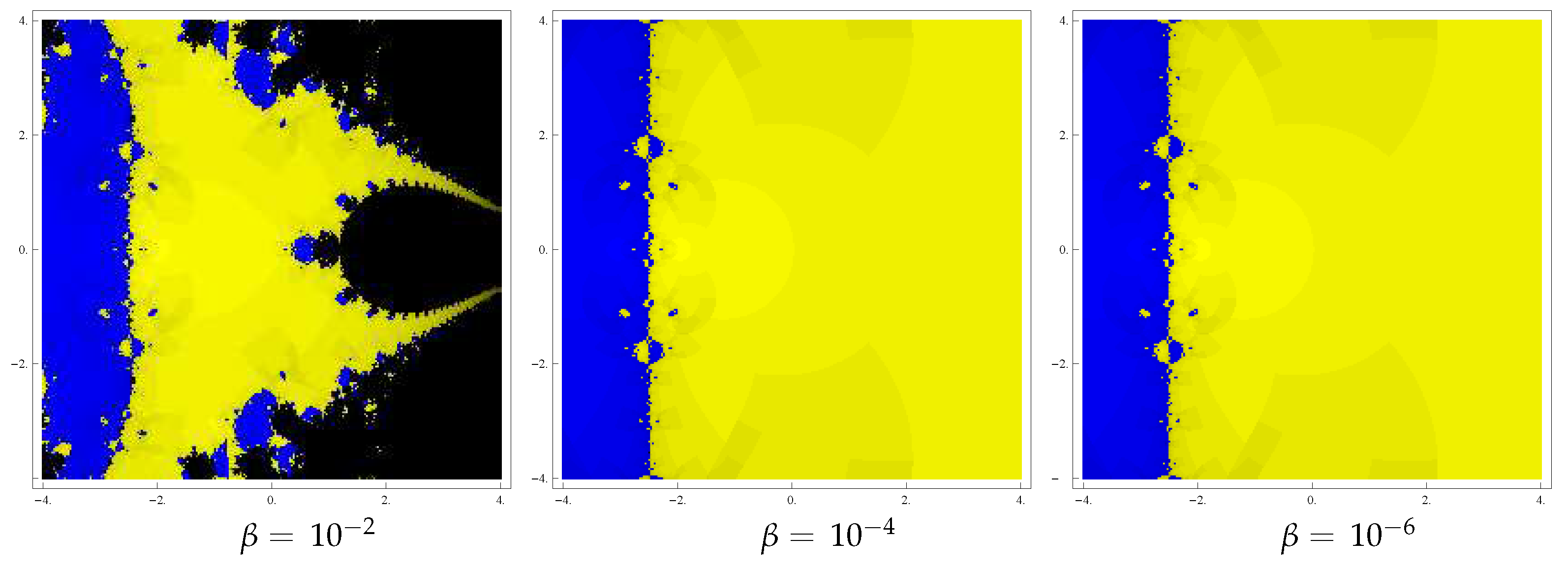
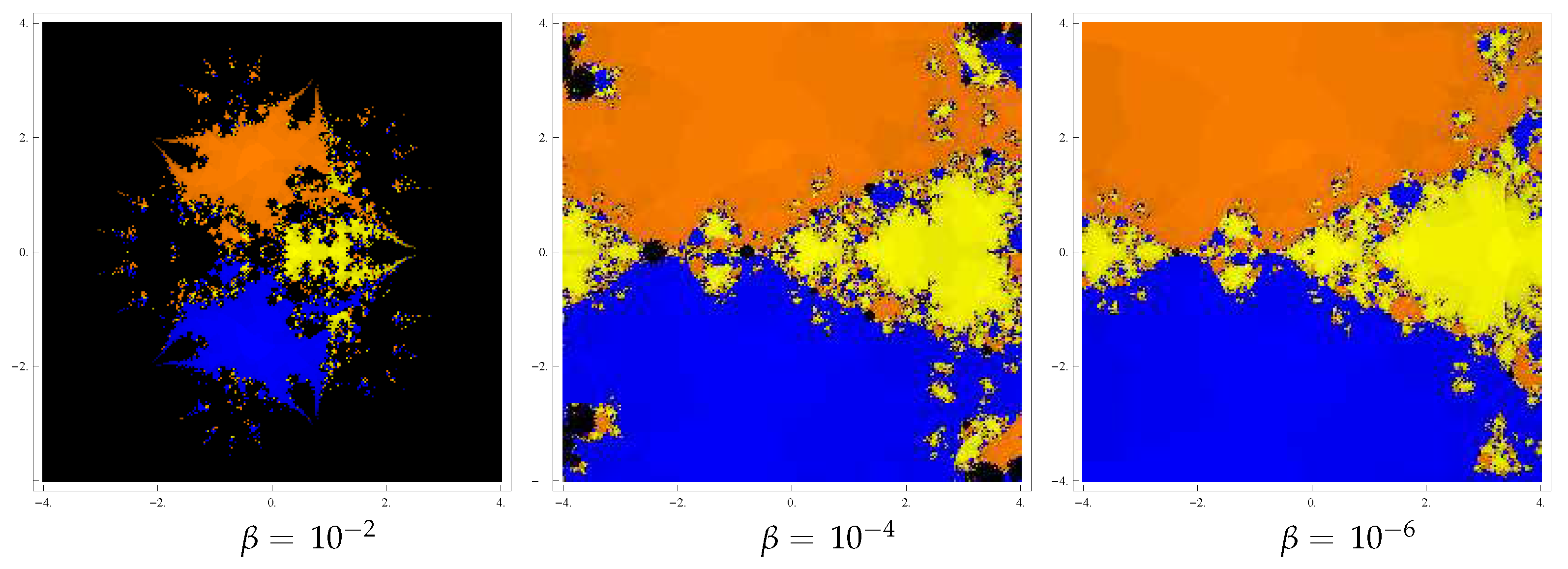
4. Basins of Attraction

Our point here is to analyze the new technique by a geometrical tool, namely the basins of attraction of the zeros of a polynomial function $P\left(z\right)$ in the Argand plane. The examination of the basins of attraction of roots by the iterative scheme gives a significant idea about the convergence of the scheme. This thought was presented in [24,25,26,27,28,29,30,31]. In order to assess the basins, we take ${10}^{-3}$ as the stopping condition for convergence, but to a maximum of 25 iterations. If this tolerance is not achieved in the required iterations, the procedure is dismissed with the result showing the divergence of the iteration function starting from $z_0$. While drawing the basins, the following criterion is adopted: a color is allotted to every initial guess $z_0$ in the attraction basin of a zero. If the iterative formula beginning at the point $z_0$ converges, then it forms the basins of attraction with that assigned color, and if the formula fails to converge in the required number of iterations, then it is painted with black color.

We discuss the basins of attraction by applying the method (26) (choosing $\beta ={10}^{-2},{10}^{-4},{10}^{-6}$) on the following two polynomials:

Problem 1.

In this example, we consider the polynomial $P_1\left(z\right)={(z^2+5z+6)}^2$, which has zeros $\{-3,-2\}$ with multiplicity two. For this situation, we utilize a square shape $D\in \mathbb{C}$ of size $[-4,4]\times [-4,4]$ and allot the shading of yellow and blue to each underlying point in the attraction basin of zero “$-2$” and “$-3$”. The basins obtained for the method appear in Figure 1 for the parameter values $\beta ={10}^{-2},{10}^{-4},{10}^{-6}$. Observing the behavior of Method (3), we see that the basins become more qualitative as parameter β accepts small values.

Figure 1. Basins of the new method for $P_1\left(z\right)$.

Problem 2.

Let us take the polynomial $P_2\left(z\right)={(z^2-\frac{1}{z}+2)}^3$ having zeros $\{-0.226\pm 1.467i,0.453\}$ with multiplicity three. To see the dynamical view, we consider a square $D=[-4,4]\times [-4,4]\in \mathbb{C}$ with shades of orange, yellow, and blue to each underlying point in the basins of attraction of zero “$-0.226-1.467i$”, “$-0.226-1.467i$”, and “$-0.453$”. Basins for proposed method (3) appear in Figure 2 corresponding to parameter values $\beta ={10}^{-2},{10}^{-4},{10}^{-6}$. Analyzing the shape of the basins, we see that the basins become enlarged with smaller values of parameter β.

Figure 2. Basins of the new method for $P_2\left(z\right)$.

It is clear that the attraction basins show the convergence behavior and suitability of an iterative scheme relying on the conditions. In the event that we pick a starter $z_0$ in a zone where different basins of attraction meet one another, it is difficult to foresee which root will be attained by the method that starts in $z_0$. Thus, the selection of $z_0$ in such a zone is not a wise decision. The graphics show that the dark zones and the zones with various hues are not appropriate to speculate about $z_0$ when we need to accomplish a specific root. The most alluring pictures show up when we have extremely perplexing wildernesses between basins of attraction. We close this segment with a comment that the nature of the proposed technique relies on the estimation of parameter $\beta$. The smaller the estimation of $\beta$, the better the convergence of the method.

5. Numerical Results

In order to check the performance and validity of the theoretical results, we apply the new method (NM) to solve some nonlinear problems. The theoretical fourth order of convergence is verified by using the formula of the approximate computational order of convergence (ACOC; see [32]):

$$\mathrm{ACOC}=\frac{ln|(u_{k+1}-u_k)/(u_k-u_{k-1})|}{ln|(u_k-u_{k-1})/(u_{k-1}-u_{k-2})|},\mathrm{for}\mathrm{each}k=1,2,\dots$$

(27)

The performance of NM is compared with some existing well-known optimal fourth order methods with and without derivative evaluations. For example, we consider the methods by Li-Liao-Cheng [8], Li-Cheng-Neta [7], Sharma-Sharma [9], Zhou-Chen-Song [10], Soleymani-Babajee-Lotfi [12], Kansal-Kanwar-Bhatia [15], and Sharma-Kumar-Jäntschi [20]. The methods are expressed as follows:

Li-Liao-Cheng method (LM-1):

$$\begin{array}{cc}\hfill w_k=& u_k-\frac{2m}{m+2}\frac{\mathsf{\Phi }\left(u_k\right)}{{\mathsf{\Phi }}^{\prime }\left(u_k\right)},\hfill \\ \hfill u_{k+1}=& u_k-\frac{m(m-2){\left(\frac{m}{m+2}\right)}^{-m}{\mathsf{\Phi }}^{\prime }\left(w_k\right)-m^2{\mathsf{\Phi }}^{\prime }\left(u_k\right)}{{\mathsf{\Phi }}^{\prime }\left(u_k\right)-{\left(\frac{m}{m+2}\right)}^{-m}{\mathsf{\Phi }}^{\prime }\left(w_k\right)}\frac{\mathsf{\Phi }\left(u_k\right)}{2{\mathsf{\Phi }}^{\prime }\left(u_k\right)}.\hfill \end{array}$$

Li-Cheng-Neta method (LM-2):

$$\begin{array}{cc}\hfill w_k=& u_k-\frac{2m}{m+2}\frac{\mathsf{\Phi }\left(u_k\right)}{{\mathsf{\Phi }}^{\prime }\left(u_k\right)},\hfill \\ \hfill u_{k+1}=& u_k-{\alpha }_1\frac{\mathsf{\Phi }\left(u_k\right)}{{\mathsf{\Phi }}^{\prime }\left(w_k\right)}-\frac{\mathsf{\Phi }\left(u_k\right)}{{\alpha }_2{\mathsf{\Phi }}^{\prime }\left(u_k\right)+{\alpha }_3{\mathsf{\Phi }}^{\prime }\left(w_k\right)},\hfill \end{array}$$

where

$$\begin{array}{cc}\hfill {\alpha }_1=& -\frac{1}{2}\frac{{\left(\frac{m}{m+2}\right)}^{m}m(m^4+4m^3-16m-16)}{m^3-4m+8},\hfill \\ \hfill {\alpha }_2=& -\frac{{(m^3-4m+8)}^2}{m(m^4+4m^3-4m^2-16m+16)(m^2+2m-4)},\hfill \\ \hfill {\alpha }_3=& \frac{m^2(m^3-4m+8)}{{\left(\frac{m}{m+2}\right)}^m(m^4+4m^3-4m^2-16m+16)(m^2+2m-4)}.\hfill \end{array}$$

Sharma-Sharma method (SSM):

$$\begin{array}{cc}\hfill w_k=& u_k-\frac{2m}{m+2}\frac{\mathsf{\Phi }\left(u_k\right)}{{\mathsf{\Phi }}^{\prime }\left(u_k\right)},\hfill \\ \hfill u_{k+1}=& u_k-\frac{m}{8}[(m^3-4m+8)-{(m+2)}^2{\left(\frac{m}{m+2}\right)}^m\frac{{\mathsf{\Phi }}^{\prime }\left(u_k\right)}{{\mathsf{\Phi }}^{\prime }\left(w_k\right)}\hfill \\ \hfill & \times \left(2(m-1)-(m+2){\left(\frac{m}{m+2}\right)}^m\frac{{\mathsf{\Phi }}^{\prime }\left(u_k\right)}{{\mathsf{\Phi }}^{\prime }\left(w_k\right)}\right)]\frac{\mathsf{\Phi }\left(u_k\right)}{{\mathsf{\Phi }}^{\prime }\left(u_k\right)}.\hfill \end{array}$$

Zhou-Chen-Song method (ZM):

$$\begin{array}{cc}\hfill w_k=& u_k-\frac{2m}{m+2}\frac{\mathsf{\Phi }\left(u_k\right)}{{\mathsf{\Phi }}^{\prime }\left(u_k\right)},\hfill \\ \hfill u_{k+1}=& u_k-\frac{m}{8}[m^3{\left(\frac{m+2}{m}\right)}^{2m}{\left(\frac{{\mathsf{\Phi }}^{\prime }\left(w_k\right)}{{\mathsf{\Phi }}^{\prime }\left(u_k\right)}\right)}^2-2m^2(m+3){\left(\frac{m+2}{m}\right)}^m\frac{{\mathsf{\Phi }}^{\prime }\left(w_k\right)}{{\mathsf{\Phi }}^{\prime }\left(u_k\right)}\hfill \\ \hfill & +(m^3+6m^2+8m+8)]\frac{\mathsf{\Phi }\left(u_k\right)}{{\mathsf{\Phi }}^{\prime }\left(u_k\right)}.\hfill \end{array}$$

Soleymani-Babajee-Lotfi method (SM):

$$\begin{array}{cc}\hfill w_k=& u_k-\frac{2m}{m+2}\frac{\mathsf{\Phi }\left(u_k\right)}{{\mathsf{\Phi }}^{\prime }\left(u_k\right)},\hfill \\ \hfill u_{k+1}=& u_k-\frac{{\mathsf{\Phi }}^{\prime }\left(w_k\right)\mathsf{\Phi }\left(u_k\right)}{q_1{\left({\mathsf{\Phi }}^{\prime }\left(w_k\right)\right)}^2+q_2{\mathsf{\Phi }}^{\prime }\left(w_k\right){\mathsf{\Phi }}^{\prime }\left(u_k\right)+q_3{\left({\mathsf{\Phi }}^{\prime }\left(u_k\right)\right)}^2},\hfill \end{array}$$

where

$$\begin{array}{cc}\hfill q_1=& \frac{1}{16}{m}^{3-m}{(m+2)}^m,\hfill \\ \hfill q_2=& \frac{8-m(m+2)(m^2-2)}{8m},\hfill \\ \hfill q_3=& \frac{1}{16}(m-2)m^{m-1}{(m+2)}^{3-m}.\hfill \end{array}$$

Kansal-Kanwar-Bhatia method (KM):

$$\begin{array}{cc}\hfill w_k=& u_k-\frac{2m}{m+2}\frac{\mathsf{\Phi }\left(u_k\right)}{{\mathsf{\Phi }}^{\prime }\left(u_k\right)},\hfill \\ \hfill u_{k+1}=& u_k-\frac{m}{4}\mathsf{\Phi }\left(u_k\right)\left(1+\frac{m^4{p}^{-2m}{\left(p^{m-1}-\frac{{\mathsf{\Phi }}^{\prime }\left(w_k\right)}{{\mathsf{\Phi }}^{\prime }\left(u_k\right)}\right)}^2(p^m-1)}{8(2p^m+m(p^m-1))}\right)\hfill \\ \hfill & \times \left(\frac{4-2m+m^2(p^{-m}-1)}{{\mathsf{\Phi }}^{\prime }\left(u_k\right)}-\frac{p^{-m}{(2p^m+m(p^m-1))}^2}{{\mathsf{\Phi }}^{\prime }\left(u_k\right)-{\mathsf{\Phi }}^{\prime }\left(w_k\right)}\right),\hfill \end{array}$$

where $p=\frac{m}{m+2}.$

Sharma-Kumar-Jäntschi method (SM-1):

$$\begin{array}{cc}\hfill w_k=& u_k-\frac{\mathsf{\Phi }\left(u_k\right)}{\mathsf{\Phi }[v_k,u_k]},\hfill \\ \hfill u_{k+1}=& w_k-\left(s_k+m{s}_k^2+(m-1)y_k+m{s}_k{y}_k\right)\frac{\mathsf{\Phi }\left(u_k\right)}{\mathsf{\Phi }[v_k,u_k]}.\hfill \end{array}$$

Sharma-Kumar-Jäntschi method (SM-2):

$$\begin{array}{cc}\hfill w_k=& u_k-\frac{\mathsf{\Phi }\left(u_k\right)}{\mathsf{\Phi }[v_k,u_k]},\hfill \\ \hfill u_{k+1}=& w_k+\frac{s_k+m{s}_k^2-(m-1)y_k(m{y}_k-1)}{m{y}_k-1}\frac{\mathsf{\Phi }\left(u_k\right)}{\mathsf{\Phi }[v_k,u_k]},\hfill \end{array}$$

where $y_k=\sqrt[m]{\frac{\mathsf{\Phi }\left(w_k\right)}{f\left(v_k\right)}}$.

The calculations were executed in the programmable package of the Mathematica software [23] with higher precision. The results of the new method were obtained by choosing a value of $0.01$ for the parameter $\beta$. The numerical results shown in Table 1, Table 2, Table 3 and Table 4 include: (i) the number of iterations $\left(k\right)$ that are needed to converge to the required solution such that $|u_{k+1}-u_k|+|\mathsf{\Phi }\left(u_k\right)|<{10}^{-100}$, (ii) the estimated error $|u_{k+1}-u_k|$ in the first three iterations, (iii) the approximated computational order of convergence (ACOC) using Formula (27), and (iv) the elapsed CPU time to run the program measured by the Mathematica command “TimeUsed[ ]”.

Table 1. Numerical results of the methods for ${\mathsf{\Phi }}_1\left(u\right)$. ACOC, approximate computational order of convergence; LM-1, Li-Liao-Cheng method; LM-2, Li-Cheng-Neta method; SSM, Sharma-Sharma method; ZM, Zhou-Chen-Song method; SM, Soleymani-Babajee-Lotfi method; KM, Kansal-Kanwar-Bhatia method; SM-1, Sharma-Kumar-Jäntschi method; SM-2, Sharma-Kumar-Jäntschi method; NM, new method.

Methods	k	$|{\mathit{u}}_2-{\mathit{u}}_1|$	$|{\mathit{u}}_3-{\mathit{u}}_2|$	$|{\mathit{u}}_4-{\mathit{u}}_3|$	ACOC	CPU
LM−1	6	$6.59\times {10}^{-2}$	$4.67\times {10}^{-3}$	$3.77\times {10}^{-6}$	4.000	0.0776
LM−2	6	$6.59\times {10}^{-2}$	$4.67\times {10}^{-3}$	$3.77\times {10}^{-6}$	4.000	0.0942
SSM	6	$6.72\times {10}^{-2}$	$5.05\times {10}^{-3}$	$5.32\times {10}^{-6}$	4.000	0.0782
ZM	6	$6.99\times {10}^{-2}$	$5.90\times {10}^{-3}$	$1.09\times {10}^{-5}$	4.000	0.0634
SM	6	$6.59\times {10}^{-2}$	$4.67\times {10}^{-3}$	$3.77\times {10}^{-6}$	4.000	0.0935
KM	6	$6.50\times {10}^{-2}$	$4.39\times {10}^{-3}$	$2.49\times {10}^{-6}$	4.000	0.0624
SM−1	6	$7.17\times {10}^{-2}$	$6.50\times {10}^{-3}$	$1.86\times {10}^{-5}$	4.000	0.0724
SM−2	6	$5.79\times {10}^{-2}$	$2.75\times {10}^{-3}$	$3.01\times {10}^{-7}$	4.000	0.0745
NM	5	$5.59\times {10}^{-2}$	$2.36\times {10}^{-3}$	$1.22\times {10}^{-7}$	4.000	0.0615

Table 2. Numerical results of the methods for ${\mathsf{\Phi }}_2\left(u\right)$.

Methods	k	$|{\mathit{u}}_2-{\mathit{u}}_1|$	$|{\mathit{u}}_3-{\mathit{u}}_2|$	$|{\mathit{u}}_4-{\mathit{u}}_3|$	ACOC	CPU
LM−1	4	$1.95\times {10}^{-5}$	$1.17\times {10}^{-22}$	$1.51\times {10}^{-91}$	4.000	0.8274
LM−2	4	$1.95\times {10}^{-5}$	$1.17\times {10}^{-22}$	$1.51\times {10}^{-91}$	4.000	1.1072
SSM	4	$1.95\times {10}^{-5}$	$1.17\times {10}^{-22}$	$1.53\times {10}^{-91}$	4.000	1.1076
ZM	4	$1.96\times {10}^{-5}$	$1.18\times {10}^{-22}$	$1.58\times {10}^{-91}$	4.000	1.1066
SM	4	$1.95\times {10}^{-5}$	$1.18\times {10}^{-22}$	$1.54\times {10}^{-91}$	4.000	1.2947
KM	4	$1.95\times {10}^{-5}$	$1.16\times {10}^{-22}$	$1.44\times {10}^{-91}$	4.000	1.0952
SM−1	3	$2.76\times {10}^{-6}$	$8.00\times {10}^{-27}$	0	4.000	0.3284
SM−2	3	$2.24\times {10}^{-6}$	$2.59\times {10}^{-27}$	0	4.000	0.3375
NM	3	$2.42\times {10}^{-6}$	$3.93\times {10}^{-27}$	0	4.000	0.3124

Table 3. Numerical results of the methods for ${\mathsf{\Phi }}_3\left(u\right)$.

Methods	k	$|{\mathit{u}}_2-{\mathit{u}}_1|$	$|{\mathit{u}}_3-{\mathit{u}}_2|$	$|{\mathit{u}}_4-{\mathit{u}}_3|$	ACOC	CPU
LM−1	4	$1.07\times {10}^{-3}$	$1.14\times {10}^{-14}$	$1.46\times {10}^{-58}$	4.000	1.6382
LM−2	4	$1.07\times {10}^{-3}$	$1.13\times {10}^{-14}$	$1.43\times {10}^{-58}$	4.000	1.7935
SSM	4	$1.07\times {10}^{-3}$	$1.12\times {10}^{-14}$	$1.35\times {10}^{-58}$	4.000	1.9031
ZM	4	$1.07\times {10}^{-3}$	$1.10\times {10}^{-14}$	$1.23\times {10}^{-58}$	4.000	1.8720
SM	4	$1.07\times {10}^{-3}$	$1.08\times {10}^{-14}$	$1.16\times {10}^{-58}$	4.000	1.9655
KM	4	$1.07\times {10}^{-3}$	$1.19\times {10}^{-14}$	$1.82\times {10}^{-58}$	4.000	1.9026
SM−1	4	$2.64\times {10}^{-5}$	$6.95\times {10}^{-21}$	$3.34\times {10}^{-83}$	4.000	1.4802
SM−2	4	$2.62\times {10}^{-5}$	$2.27\times {10}^{-21}$	$1.29\times {10}^{-85}$	4.000	1.4922
NM	4	$2.63\times {10}^{-5}$	$4.57\times {10}^{-21}$	$4.18\times {10}^{-84}$	4.000	1.4656

Table 4. Numerical results of the methods for ${\mathsf{\Phi }}_4\left(u\right)$.

Methods	k	$|{\mathit{u}}_2-{\mathit{u}}_1|$	$|{\mathit{u}}_3-{\mathit{u}}_2|$	$|{\mathit{u}}_4-{\mathit{u}}_3|$	ACOC	CPU
LM−1	4	$3.04\times {10}^{-4}$	$3.16\times {10}^{-15}$	$3.68\times {10}^{-59}$	4.000	1.4512
LM−2	4	$3.04\times {10}^{-4}$	$3.16\times {10}^{-15}$	$3.70\times {10}^{-59}$	4.000	2.2314
SSM	4	$3.04\times {10}^{-4}$	$3.17\times {10}^{-15}$	$3.76\times {10}^{-59}$	4.000	2.2615
ZM	4	$3.04\times {10}^{-4}$	$3.18\times {10}^{-15}$	$3.84\times {10}^{-59}$	4.000	2.3088
SM	4	$3.04\times {10}^{-4}$	$3.23\times {10}^{-15}$	$4.14\times {10}^{-59}$	4.000	2.7610
KM	4	$3.04\times {10}^{-4}$	$3.11\times {10}^{-15}$	$3.40\times {10}^{-59}$	4.000	2.2926
SM−1	4	$3.23\times {10}^{-5}$	$2.14\times {10}^{-19}$	$4.16\times {10}^{-76}$	4.000	0.7223
SM−2	4	$3.22\times {10}^{-5}$	$8.04\times {10}^{-21}$	$3.10\times {10}^{-83}$	4.000	0.7407
NM	4	$3.09\times {10}^{-5}$	$1.11\times {10}^{-19}$	$1.83\times {10}^{-77}$	4.000	0.5931

The following numerical examples were selected for testing:

Example 1.

Consider the van der Waals equation:

$$\left(P+\frac{a_1{n}^2}{V^2}\right)(V-n{a}_2)=nRT,$$

which shows the nature of a real gas by the inclusion of parameters $a_1$ and $a_2$ in the ideal gas equation. The volume V in terms of the remaining parameters can be found by the equation:

$$P{V}^3-(n{a}_{2}P+nRT)V^2+a_1{n}^{2}V-a_1{a}_2{n}^2=0.$$

For a given a set of values of $a_1$ and $a_2$ of a particular gas, one can find values of n, P, and T, so that the equation has three roots. For a particular set of values, we have:

$${\mathsf{\Phi }}_1\left(u\right)=u^3-5.22u^2+9.0825u-5.2675.$$

This function has three zeros: one is a simple zero $\alpha =1.72$ and the other is a repeated zero $\alpha =1.75$ of multiplicity two. The methods were tested for initial guess $u_0=2.3$ to find the desired zero $\alpha =1.75$. The computed results are given in Table 1.

Example 2.

Let λ, c, T, k, and h be wavelength of the radiation, the speed of light, the absolute temperature of the black body, Boltzmann’s constant, and Planck’s constant, respectively. Then, the Planck law of radiation [33] to find the energy density in a black body is given as:

$$\varphi \left(\lambda \right)=\frac{8\pi ch{\lambda }^{-5}}{e^{ch/\lambda kT}-1}.$$

(28)

One wants to determine the wavelength λ corresponding to the maximum energy density $\varphi \left(\lambda \right)$. From Equation (28), it follows that:

$${\varphi }^{\prime }\left(\lambda \right)=\left(\frac{8\pi ch{\lambda }^{-6}}{e^{ch/\lambda kT}-1}\right)\left(\frac{(ch/\lambda kT)e^{ch/\lambda kT}}{e^{ch/\lambda kT}-1}-5\right)=L.M.\left(say\right)$$

A maximum for ϕ will occur for $M=0$, that is if:

$$\frac{(ch/\lambda kT)e^{ch/\lambda kT}}{e^{ch/\lambda kT}-1}=5.$$

Setting $u=ch/\lambda kT$, the above equation assumes the form:

$$1-\frac{u}{5}=e^{-u}.$$

(29)

The following function can be obtained by considering the above case three times:

$${\mathsf{\Phi }}_2\left(u\right)={\left(e^{-u}-1+\frac{u}{5}\right)}^3.$$

(30)

The trivial zero $u=0$ is not taken for discussion. The non-trivial zero can be guessed somewhere near $u=5$, since for $u=5$, the left-hand side of (29) is zero and the right-hand side is $e^{-5}\approx 6.74\times {10}^{-3}$. In fact the expected root $\alpha \approx 4.96511423174427630369$ is obtained with the starter $u_0=5.4$. Thereby, the wavelength (λ) for the maximum energy density is:

$$\lambda \approx \frac{ch}{4.96511423174427630369\left(kT\right)}.$$

The numerical results are displayed in Table 2.

Example 3.

The problem of isentropic supersonic flow around a sharp expansion corner is considered. The mathematical expression between the Mach number before the corner (i.e., $M_1$) and after the corner (i.e., $M_2$) is defined by (see [34]):

$$\begin{array}{c}\hfill \delta =b^{1/2}\left({tan}^{-1}{\left(\frac{M_2^2-1}{b}\right)}^{1/2}-{tan}^{-1}{\left(\frac{M_1^2-1}{b}\right)}^{1/2}\right)-\left({tan}^{-1}{(M_2^2-1)}^{1/2}-{tan}^{-1}{(M_1^2-1)}^{1/2}\right),\end{array}$$

where $b=\frac{\gamma +1}{\gamma -1}$, γ being the specific heat ratio of the gas.

Given that $M_1=1.5$, $\gamma =1.4$ and $\delta ={10}^0$, we solve the equation for $M_2$. This case results in:

$${tan}^{-1}\left(\frac{\sqrt{5}}{2}\right)-{tan}^{-1}\left(\sqrt{u^2-1}\right)+\sqrt{6}\left({tan}^{-1}\left(\sqrt{\frac{u^2-1}{6}}\right)-{tan}^{-1}\left(\frac{1}{2}\sqrt{\frac{5}{6}}\right)\right)-\frac{11}{63}=0,$$

where $u=M_2$.

Let us consider this equation four times, and so, the required function is:

$$\begin{array}{c}\hfill {\mathsf{\Phi }}_3\left(u\right)={\left[{tan}^{-1}\left(\frac{\sqrt{5}}{2}\right)-{tan}^{-1}\left(\sqrt{u^2-1}\right)+\sqrt{6}\left({tan}^{-1}\left(\sqrt{\frac{u^2-1}{6}}\right)-{tan}^{-1}\left(\frac{1}{2}\sqrt{\frac{5}{6}}\right)\right)-\frac{11}{63}\right]}^4.\end{array}$$

This function possesses zero $\alpha \approx 1.8411027704926161$ with multiplicity four. The required zero is calculated using starter $u_0=1.5$. The results obtained by the methods are displayed in Table 3.

Example 4.

Lastly, the standard test function defined by:

$${\mathsf{\Phi }}_4\left(u\right)=u(u^2+1)(2e^{u^2+1}+u^2-1){cosh}^3\left(\frac{\pi u}{2}\right),$$

is considered. The function ${\mathsf{\Phi }}_4$ has multiple imaginary zero $\alpha =i$ of multiplicity five. We select the initial value $u_0=1.3i$ to obtain the required zero of the function. The numerical results so produced are shown in Table 4.

It can be seen from the numerical results displayed in Table 1, Table 2, Table 3 and Table 4 that the proposed method supported the theoretical results proven in Section 2 and Section 3 and, like existing methods, possessed consistent convergence. Moreover, the CPU time consumed by the methods as shown in the tables proved computationally efficient nature of the new technique as compared to the CPU time of the considered existing methods of the same order. The main aim of applying the new derivative-free method on different nonlinear equations was purely to show its accuracy and consistency. Similar numerical testing, carried out for a number of problems of different types, confirmed the above conclusions to a good extent.

6. Conclusions

In the study, we proposed a derivative-free numerical method with optimal fourth order convergence for approximating the repeated roots of nonlinear equations. The analysis of the convergence under standard hypotheses proved the convergence order four. The method was employed to solve nonlinear problems including those arising from real-world applications. The performance was compared with existing techniques (with and without derivatives) of the same order. The testing of the numerical results showed the presented derivative-free method as a good competitor of the already established fourth order techniques that use derivative information in the algorithm. We conclude this work with a remark: the derivative-free method presented here can be a better choice compared to existing Newton-type schemes in the cases where derivatives are difficult to obtain or expensive to compute.

References

- Tetsuro, Y. Historical Developments in Convergence Analysis for Newton’s and Newton-Like Methods. In Numerical Analysis: Historical Developments in the 20th Century; Brezinski, C., Wuytack, L., Eds.; Elsevier: Amsterdam, The Netherlands, 2001; pp. 241–263. [Google Scholar]
- Kantorovich, L.V. On Newton’s Method. In Collected Works on Approximation Analysis of the Leningrad Branch of the Institute; Trudy Mat. Inst. Steklov.; Academy of Sciences of the Soviet Union: Moscow, Russia, 1949; pp. 104–144. [Google Scholar]
- Argyros, I.K. Convergence and Applications of Newton-Type Iterations; Springer: New York, NY, USA, 2008. [Google Scholar]
- Schröder, E. Über unendlich viele Algorithmen zur Auflösung der Gleichungen. Math. Ann. 1870, 2, 317–365. [Google Scholar] [CrossRef]
- Hansen, E.; Patrick, M. A family of root finding methods. Numer. Math. 1977, 27, 257–269. [Google Scholar] [CrossRef]
- Dong, C. A family of multipoint iterative functions for finding multiple roots of equations. Int. J. Comput. Math. 1987, 21, 363–367. [Google Scholar] [CrossRef]
- Li, S.; Liao, X.; Cheng, L. A new fourth-order iterative method for finding multiple roots of nonlinear equations. Appl. Math. Comput. 2009, 215, 1288–1292. [Google Scholar]
- Li, S.G.; Cheng, L.Z.; Neta, B. Some fourth-order nonlinear solvers with closed formulae for multiple roots. Comput. Math. Appl. 2010, 59, 126–135. [Google Scholar] [CrossRef]
- Sharma, J.R.; Sharma, R. Modified Jarratt method for computing multiple roots. Appl. Math. Comput. 2010, 217, 878–881. [Google Scholar] [CrossRef]
- Zhou, X.; Chen, X.; Song, Y. Constructing higher-order methods for obtaining the multiple roots of nonlinear equations. J. Comput. Appl. Math. 2011, 235, 4199–4206. [Google Scholar] [CrossRef]
- Sharifi, M.; Babajee, D.K.R.; Soleymani, F. Finding the solution of nonlinear equations by a class of optimal methods. Comput. Math. Appl. 2012, 63, 764–774. [Google Scholar] [CrossRef]
- Soleymani, F.; Babajee, D.K.R.; Lotfi, T. On a numerical technique for finding multiple zeros and its dynamics. J. Egypt. Math. Soc. 2013, 21, 346–353. [Google Scholar] [CrossRef]
- Geum, Y.H.; Kim, Y.I.; Neta, B. A class of two-point sixth-order multiple-zero finders of modified double-Newton type and their dynamics. Appl. Math. Comput. 2015, 270, 387–400. [Google Scholar] [CrossRef]
- Geum, Y.H.; Kim, Y.I.; Neta, B. Constructing a family of optimal eighth-order modified Newton-type multiple-zero finders along with the dynamics behind their purely imaginary extraneous fixed points. J. Comp. Appl. Math. 2018, 333, 131–156. [Google Scholar] [CrossRef]
- Kansal, M.; Kanwar, V.; Bhatia, S. On some optimal multiple root-finding methods and their dynamics. Appl. Appl. Math. 2015, 10, 349–367. [Google Scholar]
- Behl, R.; Alsolami, A.J.; Pansera, B.A.; Al-Hamdan, W.M.; Salimi, M.; Ferrara, M. A new optimal family of Schrder’s method for multiple zeros. Mathematics 2019, 7, 1076. [Google Scholar] [CrossRef]
- Behl, R.; Salimi, M.; Ferrara, M.; Sharifi, S.; Alharbi, S.K. Some real-life applications of a newly constructed derivative free iterative scheme. Symmetry 2019, 11, 239. [Google Scholar] [CrossRef]
- Traub, J.F. Iterative Methods for the Solution of Equations; Chelsea Publishing Company: New York, NY, USA, 1982. [Google Scholar]
- Kumar, D.; Sharma, J.R.; Argyros, I.K. Optimal one-point iterative function free from derivatives for multiple roots. Mathematics 2020, 8, 709. [Google Scholar] [CrossRef]
- Sharma, J.R.; Kumar, S.; Jäntschi, L. On a class of optimal fourth order multiple root solvers without using derivatives. Symmetry 2019, 11, 1452. [Google Scholar] [CrossRef]
- Sharma, J.R.; Kumar, S.; Argyros, I.K. Development of optimal eighth order derivative-free methods for multiple roots of nonlinear equations. Symmetry 2019, 11, 766. [Google Scholar] [CrossRef]
- Kung, H.T.; Traub, J.F. Optimal order of one-point and multipoint iteration. J. Assoc. Comput. Mach. 1974, 21, 643–651. [Google Scholar] [CrossRef]
- Wolfram, S. The Mathematica Book, 5th ed.; Wolfram Media: Champaign, IL, USA, 2003. [Google Scholar]
- Vrscay, E.R.; Gilbert, W.J. Extraneous fixed points, basin boundaries and chaotic dynamics for Schröder and König rational iteration functions. Numer. Math. 1988, 52, 1–16. [Google Scholar] [CrossRef]
- Varona, J.L. Graphic and numerical comparison between iterative methods. Math. Intell. 2002, 24, 37–46. [Google Scholar] [CrossRef]
- Jézéquel, F. Dynamical Control of Approximation Methods; Habilitationa diriger des recherches, Universit Pierre et Marie Curie: Paris, France, 2005. [Google Scholar]
- Chand, P.B.; Chicharro, F.I.; Jain, P. Optimal fourth-order Weerakoon-Fernando-type methods for multiple roots and their dynamics. Mediterr. J. Math. 2019, 16, 67. [Google Scholar] [CrossRef]
- Geum, Y.H.; Kim, Y.I.; Magreñán, Á.A. A study of dynamics via Möbius conjugacy map on a family of sixth-order modified Newton-like multiple-zero finders with bivariate polynomial weight functions. J. Comput. Appl. Math. 2018, 344, 608–623. [Google Scholar] [CrossRef]
- Behl, R.; Cordero, A.; Motsa, S.; Torregrosa, J.R. On developing fourth-order optimal families of methods for multiple roots and their dynamics. Appl. Math. Comput. 2018, 265, 520–532. [Google Scholar] [CrossRef]
- Sidorov, N.; Sidorov, D.; Li, Y. Basins of attraction and stability of nonlinear systems’ equilibrium points. Differ. Equ. Dyn. Syst. 2019. [Google Scholar] [CrossRef]
- Neta, B.; Scott, M.; Chun, C. Basin attractors for various methods for multiple roots. App. Math. Comp. 2012, 218, 5043–5066. [Google Scholar] [CrossRef]
- Cordero, A.; Torregrosa, J.R. Variants of Newtons method using fifth order quadrature formulas. Appl. Math. Comput. 2007, 190, 686–698. [Google Scholar]
- Bradie, B. A Friendly Introduction to Numerical Analysis; Pearson Education Inc.: New Delhi, India, 2006. [Google Scholar]
- Hoffman, J.D. Numerical Methods for Engineers and Scientists; McGraw-Hill Book Company: New York, NY, USA, 1992. [Google Scholar]
© 2020 by the authors. Licensee MDPI, Basel, Switzerland. This article is an open access article distributed under the terms and conditions of the Creative Commons Attribution (CC BY) license (http://creativecommons.org/licenses/by/4.0/).