Symmetric MHD Channel Flow of Nonlocal Fractional Model of BTF Containing Hybrid Nanoparticles

Abstract

A nonlocal fractional model of Brinkman type fluid (BTF) containing a hybrid nanostructure was examined. The magnetohydrodynamic (MHD) flow of the hybrid nanofluid was studied using the fractional calculus approach. Hybridized silver (Ag) and Titanium dioxide (TiO₂) nanoparticles were dissolved in base fluid water (H₂O) to form a hybrid nanofluid. The MHD free convection flow of the nanofluid (Ag-TiO₂-H₂O) was considered in a microchannel (flow with a bounded domain). The BTF model was generalized using a nonlocal Caputo-Fabrizio fractional operator (CFFO) without a singular kernel of order $\alpha$ with effective thermophysical properties. The governing equations of the model were subjected to physical initial and boundary conditions. The exact solutions for the nonlocal fractional model without a singular kernel were developed via the fractional Laplace transform technique. The fractional solutions were reduced to local solutions by limiting $\alpha \to 1$. To understand the rheological behavior of the fluid, the obtained solutions were numerically computed and plotted on various graphs. Finally, the influence of pertinent parameters was physically studied. It was found that the solutions were general, reliable, realistic and fixable. For the fractional parameter, the velocity and temperature profiles showed a decreasing trend for a constant time. By setting the values of the fractional parameter, excellent agreement between the theoretical and experimental results could be attained.

1. Introduction

In thermal transport systems, the poor thermophysical properties of various working fluids can be improved by the addition of nanometer-sized particles. This technique leads to an improvement in the thermal conductivity of the working fluid, making it more reliable and long-lasting. The resulting new class of fluids refers to nanofluids with a broad range of applications in different fields of science and engineering, including nuclear reactors, solar panels, heat exchangers, biological and chemical instruments, and automobile radiators [1,2,3,4,5,6]. When the nanofluid is used in automobile radiators, the fluid consumption was reduced by more than 5% [7]. Originally, the idea of nanofluids was presented by Choi and Eastman in 1995 [8]. Mohain et al. [9], in their review paper part I, presented the fundamental concept and discussed recent innovations in order to facilitate comprehension of the modeling of nanofluids. In this paper, they focused on recent advancements in the literature, with a detailed explanation of the thermophysical properties, modeling and simulation of heat transport in the flow of nanofluids. Furthermore, they highlighted the main challenges which still exist in this field. In the part II of their paper, Mahain et al. [10] emphasized 2D and 3D modeling in a wide range of geometries with different numerical approaches. Finally, they provided a detailed list of applications for nanofluids in different fields of science and engineering, with useful future directions and suggestions.

Nanofluids have received a great deal of attention from researchers due to their enhanced heat transport properties. But this should not be their only application; viscosity also plays a vital role in the efficiency of nanofluids in the convection processes. Vallejo et al. [11] studied the rheological behavior of a graphene nanofluid by means of a rotational rheometer. They found that the nanofluid behaved as a non-Newtonian shear thinning liquid at a specific temperature and with a specific ratio of water and propylene glycol. In another paper, Vallejo et al. [12] investigated the the rheological properties of six carbon-based nonliquids. An ethylene glycol-based $S{i}_3{N}_4$ nanofluid was experimentally studied by Żyła et al. [13]. They found that in the UV region, the absorption of the nanofluid increased by increasing the volume concentration of the nanoparticles. Fal [14,15], Murshed [16] and Estellé [17] have also contributed to the literature of nanofluids. Nanofluids have been widely studied in by the research community and which has led to numerous achievements. Nanofluids have been classified in many classes, in which the most lately is hybrid nanofluids [18]. Hybrid nanofluids are the mixture of two unlike nanoparticles in the base fluid. The primary incentive of hybrid nanofluid is to additionally improve thermal characteristics of nanofluids. In coaction to this Izadi et al. [19] studied variable heat transfer of hybrid nanofluid under the impact of external magnetic field. The advanced heat transfer in non-Newtonian hybrid nanofluid together with entropy generation was analyzed by Shahsavar et al. [20]. The convective flow of hybrid nanofluid inside a cavity along with entropy generation was studied by Hussain et al. [20]. Furthermore, Farooq et al. [21] investigated entropy generation in the flow of hybrid nanofluid over nonlinear stretching surface.

In 2018, the concept of fractional derivatives was 323 years old. But over the last 55 years, i.e., since the work of Caputo [22] in 1967, this field has received considerable attention from researchers. Caputo was the first mathematician to develop the fractional operator by using Laplace convolutions production of power-law functions and fractional derivatives. This was the first fractional operator to fix the problem of the Riemann–Liouville fractional operator (RLFO), i.e., the problem of atypical initial conditions with no real meaning which are complicated to handle. In the literature, the Caputo fractional operator (CFO) and RLFO are widely used in various fields of science [23,24]; however, the kernel of these fractional operators is singular at $t=\tau$, which leads to some erroneous results. Fractional Calculus was further developed, and in 2015, Caputo and Fabrizio presented the Caputo-Fabrizio fractional operator (CFFO) with a nonsingular exponential kernel. [25]. This new fractional operator has been successfully employed in a variety of real situations. Among them, Ali et al. [26] applied CFFO to the mixed convection flow of a viscoelastic fluid near an infinite vertical parallel plate. Sheikh et al. [27] employed CFFO to study magneto-hydrodynamic (MHD) convective flow through an infinitely flat plate. Zafar and Fetecau [28] used CFFO and present new solutions for the flow of a viscous fluid near a static vertical plate. Hristov [29] dedicated a chapter to CFFO. He claimed that CFFO naturally appears in the diffusion equation as the relaxation term when the constitutive equation relating the flux and the gradient contains either the Jeffrey kernel or the Cattaneo exponential kernel. Atangana and Koca [30] analyzed a nonlinear Baggs and Freedman using Caputo-Fabrizio fractional derivative with special solutions using an iterative method. However, CFFO has also been criticized by the research community. The main concerns about it were: (1) The solution of ${}^{CF}{D}_t^{a}g(y,t)=-ag\left(y,t\right)$ is an exponential equation, not an exponential function; (2) The kernel CFFO is nonsingular but local; and (3) CFFO is the average of the function and its integral, not a fractional operator. To address this shortcoming, Atangana and Baleanu came up with new approach by introducing the Atanagana-Baleanu fractional operator (ABFO). The kernel of ABFO is a nonlocal and nonsingular Mittag-Leffler function [31]. This new operator satisfies all the properties of a fractional derivate except index law. Caputo and Fabrizio [32] responded that the definition presented in [25] satisfied all the general properties of fractional derivatives including nonlocality. Recently, Hristov [33] demonstrated the viscoelastic response functions and their relationship with the Caputo-Fabrizio fractional derivative, and addressed the criticism of [25]. The response of Caputo and Fabrizio and Hristov was appreciated by many researchers, and has been widely accepted. Hence, presently, both ABFO and CFFO are in practice.

To the best of the authors’ knowledge, no study has been published on nonlocal Brinkman-type hybrid nanofluids in a microchannel. Therefore, there is a need to fill this gap by studying hybrid nanofluids with a nonlocal fractional derivative. Hence, this article seeks to combine the idea of nonlocal fractional derivatives and hybrid nanofluids. For this purpose, a nonlocal Brinkman type fluid model with the thermophysical properties of a hybrid nanofluid was developed. The exact solutions for the model were obtained via the Laplace transform technique. The influence of various flow parameters was studied through numerical computation and graphical representation.

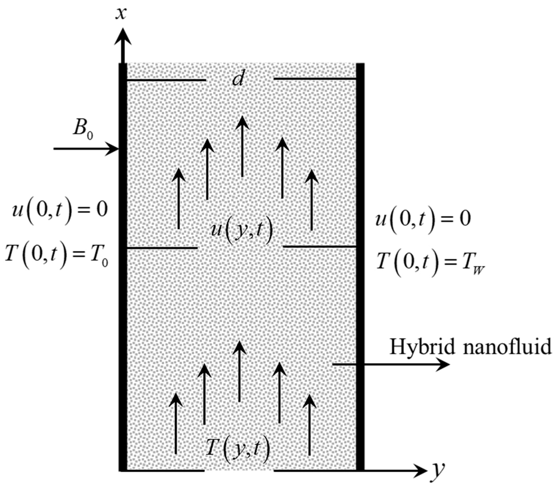
2. Description of the Problem

Assume that MHD natural convection flow occurs in the microchannel of a generalized, electrically conductive $Ag-Ti{O}_2-H_{2}O$ hybrid nanofluid. In the length, the microchannel is considered infinite with width $d$. The channel is parallel to the $x-$axis where the $y-$axis is perpendicular to it. It is assumed that at $t\le 0$, the system is at rest at room temperature, $T_0$. After $t=0^{+}$, the temperature rises from $T_0$ to $T_W$. The natural convection occurs because of the temperature gradient that increases the buoyancy forces. Hence, fluid accelerates in the $x-$direction. A magnetic field of magnitude $B_0$ employed transversely to the flow direction is represented in Figure 1.

The flow of the electrically conductive $Ag-Ti{O}_2-H_{2}O$ hybrid nanofluid undergoes electromotive force, which produces current. The induced magnetic field is disregarded due to the assumption of a very small Reynold number. The electromagnetic force hinges on the intensity of electric flux [34]. The proposed problem is governed by momentum, energy and the Maxwell set of equations, which are as follows:

$$\begin{array}{l}\nabla .\mathbf{B}=0,\\ \nabla \times \mathbf{E}=-\frac{\partial \mathbf{B}}{\partial t},\\ \nabla \times \mathbf{B}={\mu }_0\mathbf{J},\end{array}\},$$

(1)

where $\mathbf{B}$, ${\mu }_0$, $\mathbf{E}$ and $\mathbf{J}$ are the magnetic flux intensity, magnetic permeability, electric field intensity and the current density, respectively. The boldface represents vectors. The relation between the Maxwell equation and generalized Ohm’s law is given by

$$\mathbf{J}={\sigma }_0[\mathbf{E}+\mathbf{V}\times \mathbf{B}]$$

(2)

where ${\sigma }_0$ and $\mathbf{V}$ are the electrical conductivity and the velocity field, respectively. The electromagnetic force is given by

$${\mathbf{F}}_{em}=\mathbf{J}\times \mathbf{B}={\sigma }_0[\mathbf{E}+\mathbf{V}\times \mathbf{B}]\times \mathbf{B}=-\sigma B_0^{2}u\left(r,t\right)\mathbf{i}$$

(3)

where $\mathbf{i}$ is a unit vector in the $x-$direction and $\mathbf{V}=\left(u\left(r,t\right)\mathbf{i},0,0\right)$ is the velocity component of the hybrid nanofluid. The electromagnetic force ${\mathbf{F}}_{em}$ is incorporated into the momentum equation of the natural convection flow of an incompressible $Ag-Ti{O}_2-H_{2}O$ hybrid nanofluid in the absence of a pressure gradient and a transverse magnetic field is applied, taking the following form [35]

$${\rho }_{hnf}\left(\frac{\partial u\left(y,t\right)}{\partial t}+{\beta }_b{}^{*}u\left(y,t\right)\right)={\mu }_{hnf}\frac{{\partial }^{2}u\left(y,t\right)}{\partial y^2}-{\sigma }_{hnf}{B}_0{}^2+g{\left(\rho {\beta }_T\right)}_{hnf}\left(T\left(y,t\right)-T_0\right),$$

(4)

$${\left(\rho Cp\right)}_{hnf}\frac{\partial T\left(y,t\right)}{\partial t}=k_{hnf}\frac{{\partial }^{2}T\left(y,t\right)}{\partial y^2}+Q_0\left(T-T_0\right),$$

(5)

subject to the given initial and natural convections and isothermal boundary conditions

$$u\left(y,0\right)=0,T\left(y,0\right)=T_0,\forall y\ge 0,$$

(6)

$$\begin{array}{l}u\left(0,t\right)=0,T\left(0,t\right)=T_0,\mathrm{For}t>0,\\ u\left(d,t\right)=0,T\left(d,t\right)=T_W,\mathrm{For}t>0,\end{array}\},$$

(7)

where ${\rho }_{hnf}$, $u\left(y,t\right)$, ${\beta }_b{}^{*}$, ${\mu }_{hnf}$, ${\sigma }_{hnf}$, $B_0$, ${\beta }_{hnf}$, ${\left(C_p\right)}_{hnf}$, $T\left(y,t\right)$ and $k_{hnf}$ are the density, velocity, Brinkmann parameter, dynamic viscosity, electrical conductivity, magnetic field, thermal expansion, specific heat, temperature and thermal conductivity, respectively.

3. Thermophysical Properties of Hybrid Nanofluid

This section presents the thermophysical properties of conventional and hybrid nanofluids. The mathematical expressions for the effective thermophysical properties of conventional nanofluids are abundantly used in the literature.

The mathematical expression for density was developed by Aminossadati and Ghasemi [36]. Brinkman [37] introduced the formula for calculating the effective dynamic viscosity of conventional nanofluids. Bourantas and Loukopoulos [38] developed mathematical expressions for volumetric thermal expansion and heat capacitance. The expression for thermal and electrical conductivities was presented by Maxwell [39,40]. To study the rheological behavior of nanofluids, Tiwari and Das [41] used these expressions. But to develop mathematical expressions to determine the thermophysical properties of a hybrid nanofluid was a challenging task, as hybrid nanofluids are a physical combination of two or more dissimilar nanoparticles in a single base fluid. The main objective of formulating hybrid nanofluids is to enhance the thermophysical properties. In many papers, different mathematical expressions have been suggested, but were not acceptable to all because, with ${\varphi }_{Ag}=0\mathrm{or}{\varphi }_{Ti{O}_2}=0$, the expressions were not reduceable, especially those regarding electrical and thermal conductivity [42]. In this manuscript, a hybrid nanofluid is characterized by $Ag$, $Ti{O}_2$ and $H_{2}O$ with ${\varphi }_{hnf}$, i.e., with a volume concentration of hybrid nanoparticles such that ${\varphi }_{hnf}={\varphi }_{Ag}+{\varphi }_{Ti{O}_2}$. The Tiwari and Das model was modified here for the hybrid nanofluid. It is worth mentioning that by making ${\varphi }_{Ag}=0\mathrm{or}{\varphi }_{Ti{O}_2}=0$, the modified model can be successfully reduced to nanofluid expressions. The numerical values of the thermophysical properties of the nanoparticles and base fluid are presented in

Table 1. Values of thermophysical properties of base fluid and nanoparticles.

Material	Base fluid	Nanoparticles
	${\mathit{H}}_2\mathit{O}$	$\mathit{T}\mathit{i}{\mathit{O}}_2$	$\mathit{A}\mathit{g}$
$\rho \left(\mathrm{kg}/{\mathrm{m}}^3\right)$	997.1	425	10500
$C_p\left(\mathrm{J}/\mathrm{kg}\mathrm{K}\right)$	4179	6862	235
$K\left(\mathrm{W}/\mathrm{m}\mathrm{K}\right)$	0.613	8.9538	429
${\beta }_T\times {10}^{-5}(K^{-1})$	21	0.9	1.89
$\sigma$	0.05	$1\times {10}^{-12}$	$3.60\times {10}^7$
Pr	6.2	-	-

, and the expression can be found in

Table 2. Expressions of nanofluid and hybrid nanofluid [42].

Thermophysical Properties	Nanofluid	Hybrid Nanofluid
Density	${\rho }_{nf}=\left(1-\varphi \right){\rho }_f+\varphi {\rho }_s,$	${\rho }_{hnf}=\left(1-{\varphi }_{hnf}\right){\rho }_f+{\varphi }_{Ag}{\rho }_{Ag}+{\varphi }_{Ti{O}_2}{\rho }_{Ti{O}_2},$
Dynamic viscosity	${\mu }_{nf}=\frac{{\mu }_f}{{\left(1-\varphi \right)}^{2.5}},$	${\mu }_{hnf}=\frac{{\mu }_f}{{\left\{1-\left({\varphi }_{Ag}+{\varphi }_{Ti{O}_2}\right)\right\}}^{2.5}}$
Thermal expansion	${\left({\beta }_T\rho \right)}_{nf}=\left(1-\varphi \right){\left({\beta }_T\rho \right)}_f+\varphi {\left({\beta }_T\rho \right)}_s$	${\left(\rho {\beta }_T\right)}_{hnf}=\left(1-{\varphi }_{hnf}\right){\left(\rho {\beta }_T\right)}_f+{\varphi }_{Ag}{\left(\rho {\beta }_t\right)}_{Ag}+{\varphi }_{Ti{O}_2}{\left(\rho {\beta }_T\right)}_{Ti{O}_2}$
Heat Capacitance	${\left(\rho C_p\right)}_{nf}=\left(1-\varphi \right){\left(\rho C_p\right)}_f+\varphi {\left(\rho C_p\right)}_s$	${\left(\rho Cp\right)}_{hnf}=\left(1-{\varphi }_{hnf}\right){\left(\rho Cp\right)}_f+{\varphi }_{Ag}{\left(\rho Cp\right)}_{Ag}+{\varphi }_{Ti{O}_2}{\left(\rho Cp\right)}_{Ti{O}_2}$
Electrical conductivity	$\frac{{\sigma }_{nf}}{{\sigma }_f}=1+\frac{3\left(\frac{{\sigma }_s}{{\sigma }_f}-1\right)\varphi }{\left(\frac{{\sigma }_s}{{\sigma }_f}+2\right)-\left(\frac{{\sigma }_s}{{\sigma }_f}-1\right)\varphi }$	$\frac{{\sigma }_{hnf}}{{\sigma }_f}=1+\frac{3\left(\frac{+{\varphi }_{Ag}{\sigma }_{Ag}+{\varphi }_{Ti{O}_2}{\sigma }_{Ti{O}_2}}{{\sigma }_f}-\varphi \right)}{\left(\frac{{\varphi }_{Ag}{\sigma }_{Ag}+{\varphi }_{Ti{O}_2}{\sigma }_{Ti{O}_2}}{\varphi {\sigma }_f}+2\right)-\left(\frac{{\varphi }_{Ag}{\sigma }_{Ag}+{\varphi }_{Ti{O}_2}{\sigma }_{Ti{O}_2}}{{\sigma }_f}-\varphi \right)}$
Thermal conductivity	$\frac{K_{nf}}{K_f}=\frac{k_s+2k_f-2\varphi \left(k_s-k_f\right)}{k_s+2k_f+\varphi \left(k_s-k_f\right)},$	$\frac{k_{hnf}}{k_f}=\frac{\frac{{\varphi }_{Ag}{k}_{Ag}+{\varphi }_{Ti{O}_2}{k}_{Ti{O}_2}}{{\varphi }_{hnf}}+2k_f+2\left({\varphi }_{Ag}{k}_{Ag}+{\varphi }_{Ti{O}_2}{k}_{{}_{Ti{O}_2}}\right)-2k_f{\varphi }_{hnf}}{\frac{{\varphi }_{Ag}{k}_{Ag}+{\varphi }_{Ti{O}_2}{k}_{Ti{O}_2}}{{\varphi }_{hnf}}+2k_f+\left({\varphi }_{Ag}{k}_{Ag}+{\varphi }_{Ti{O}_2}{k}_{{}_{Ti{O}_2}}\right)-k_f{\varphi }_{hnf}}$

[21,43,44].

4. Problem Solutions and Dimensionless Analysis

This section presents the solutions of the proposed problem using the Laplace transform method. Firstly, the system is reduced to a dimensionless form by which the following dimensionless variables

$$v=\frac{d}{{\nu }_f}u,\xi =\frac{y}{d},\tau =\frac{{\nu }_f}{d^2}t,\theta =\frac{T-T_0}{T_W-T_0},$$

are introduced into Equations (3)–(5) to yield:

$$a_0\left\{\frac{\partial v\left(\xi ,\tau \right)}{\partial \tau }+{\beta }_{b}v\left(\xi ,\tau \right)\right\}=a_1\frac{{\partial }^{2}v\left(\xi ,\tau \right)}{\partial {\xi }^2}-a_{2}M+a_{3}Gr\theta \left(\xi ,\tau \right),$$

(8)

$$a_4\mathrm{Pr}\frac{\partial \theta \left(\xi ,\tau \right)}{\partial \tau }={\lambda }_{hnf}\frac{{\partial }^2\theta \left(\xi ,\tau \right)}{\partial {\xi }^2}+Q\theta \left(\xi ,\tau \right),$$

(9)

$$v\left(\xi ,0\right)=0,\theta \left(\xi ,0\right)=0,\forall \xi \ge 0,$$

(10)

$$\begin{array}{l}v\left(0,\tau \right)=0,\theta \left(0,\tau \right)=0,\mathrm{for}\tau >0,\\ v\left(1,\tau \right)=0,\theta \left(1,\tau \right)=1,\mathrm{for}t>0,\end{array}\},$$

(11)

where

$$\begin{gathered} {\beta }_b=\frac{d^2{\beta }_b{}^{*}}{{\nu }_f{}^2},M=\frac{{\sigma }_f{d}^2{B}_0{}^2}{{\mu }_f},Gr=\frac{d^{3}g{\left({\beta }_T\right)}_f}{{\nu }_f{}^2}\left(T_W-T_0\right),\mathrm{Pr}=\frac{{\left(\mu C_p\right)}_f}{k_f},Q=\frac{d^2{Q}_0}{k_f},{\lambda }_{hnf}=\frac{k_{hnf}}{k_f},a_3=\frac{{\sigma }_{hnf}}{{\sigma }_f}, \\ {a}_0=\left(1-\varphi \right)+\frac{{\varphi }_{A{l}_2{O}_3}{\rho }_{A{l}_2{O}_3}+{\varphi }_{Cu}{\rho }_{Cu}}{{\rho }_f},a_1=\frac{1}{{\left\{1-\left({\varphi }_{A{l}_2{O}_3}+{\varphi }_{Cu}\right)\right\}}^{2.5}},a_3=\left(1-\varphi \right)+\frac{{\varphi }_{A{l}_2{O}_3}{\left(\rho {\beta }_t\right)}_{A{l}_2{O}_3}+{\varphi }_{Cu}{\left(\rho {\beta }_T\right)}_{Cu}}{{\left(\rho {\beta }_T\right)}_f}, \\ {a}_4=\left(1-\varphi \right)+\frac{{\varphi }_{A{l}_2{O}_3}{\left(\rho Cp\right)}_{A{l}_2{O}_3}+{\varphi }_{Cu}{\left(\rho Cp\right)}_{Cu}}{{\left(\rho Cp\right)}_f}, \end{gathered}$$

are the Brinkman parameter, magnetic parameter, thermal Grashof number Prandtl number and heat generation parameter, respectively. ${\lambda }_{hnf},a_0,$$a_1,a_2,a_3$ $\mathrm{and}{a}_4$ are the constants terms. The time-fractional model in terms of Caputo-Fabrizio time-fractional derivatives is as follows:

$$\frac{a_0}{a_1}{}^{CF}{D}_{\tau }{}^{\alpha }v\left(\xi ,\tau \right)+\frac{a_0}{a_1}{\beta }_{b}v\left(\xi ,\tau \right)=\frac{{\partial }^{2}v\left(\xi ,\tau \right)}{\partial {\xi }^2}-\frac{a_2}{a_1}M+\frac{a_3}{a_1}Gr\theta \left(\xi ,\tau \right),$$

(12)

$$a_3{\mathrm{Pr}}^{CF}{D}_{\tau }{}^{\beta }\theta \left(\xi ,\tau \right)={\lambda }_{hnf}\frac{{\partial }^2\theta \left(\xi ,\tau \right)}{\partial {\xi }^2}+Q\theta \left(\xi ,\tau \right),$$

(13)

where ${}^{CF}{D}_{\tau }{}^{\alpha }v\left(\xi ,\tau \right)$ and ${}^{CF}{D}_{\tau }{}^{\alpha }\theta \left(\xi ,\tau \right)$ are CFFO operators defined by [25]:

$${}^{CF}{D}_t{}^{\delta }f\left(t\right)=\frac{N\left(\delta \right)}{1-\delta }{\displaystyle \underset{0}{\overset{t}{\int }}\exp \left(-\frac{\delta \left(t-\tau \right)}{1-\delta }\right)}\frac{\partial f\left(\tau \right)}{\partial \tau }d\tau ;0<\delta <1,$$

(14)

such that

$$N\left(1\right)=N\left(0\right)=1$$

(15)

with Laplace transform:

$$ℒ\left\{{}^{CF}{D}_t{}^{\delta }f\left(t\right)\right\}\left(q\right)=\frac{q\overline{f}\left(q\right)-f\left(0\right)}{\left(1-\delta \right)q+\delta },0<\delta <1,$$

(16)

and

$$\underset{\delta \to 1}{\lim }\left[ℒ\left\{{}^{CF}{D}_t{}^{\delta }f\left(t\right)\right\}\left(q\right)\right]=\underset{\delta \to 1}{\lim }\left\{\frac{q\overline{f}\left(q\right)-f\left(0\right)}{\left(1-\delta \right)q+\delta }\right\}=q\overline{f}\left(q\right)-f\left(0\right)=ℒ\left\{\frac{\partial f\left(t\right)}{\partial t}\right\}$$

(17)

4.1. Solutions of the Energy Equation

Applying the Laplace transform to Equation (13) using Equations (14)–(17) and the corresponding initial condition from Equation (10) yields

$$a_{{}_4}\mathrm{Pr}\frac{q\theta \left(\xi ,q\right)-\theta \left(\xi ,0\right)}{\left(1-\alpha \right)q+\alpha }={\lambda }_{hnf}\frac{d^2\overline{\theta }\left(\xi ,q\right)}{\partial {\xi }^2}+Q\overline{\theta }\left(\xi ,q\right);0<\alpha <1.$$

(18)

For convenience, Equation (18) can be written as:

$$\frac{d^2\overline{\theta }\left(\xi ,q\right)}{\partial {\xi }^2}-\frac{b_{4}q-b_1{b}_3}{q+b_1}=0;0<\alpha <1,.$$

(19)

where

$$b_0=\frac{1}{1-\alpha },b_1=b_0\alpha ,b_2=\frac{a_3\mathrm{Pr}}{{\lambda }_{hnf}},b_3=\frac{Q}{{\lambda }_{hnf}},b_4=b_0{b}_2-b_3.$$

The boundary conditions in the Laplace transform domain are given by

$$\begin{array}{l}\overline{v}\left(0,q\right)=0,\overline{\theta }\left(0,q\right)\\ =0,\mathrm{for}q>0,\\ \overline{v}\left(1,q\right)=0,\overline{\theta }\left(1,q\right)\\ =\frac{1}{q},\mathrm{for}q>0,\end{array}\},$$

(20)

The exact solution of Equation (19) in the Laplace transform domain using the boundary conditions from Equation (20) is given by

$$\overline{\theta }\left(\xi ,q\right)=\frac{1}{q}\left(\sinh \xi \sqrt{\frac{b_{4}q-b_1{b}_3}{q+b_1}}\right){\left(\sinh \sqrt{\frac{b_{4}q-b_1{b}_3}{q+b_1}}\right)}^{-1};0<\alpha <1.$$

(21)

Equation (21) is further simplified as:

$$\overline{\theta }\left(\xi ,q\right)={\displaystyle \sum _{n=0}^{\infty }\left(\frac{1}{q}{e}^{-\left(1+2n-\xi \right)\sqrt{\frac{b_{4}q-b_1{b}_3}{q+b_1}}}-\frac{1}{q}{e}^{-\left(1+2n+\xi \right)\sqrt{\frac{b_{4}q-b_1{b}_3}{q+b_1}}}\right)};0<\alpha <1.$$

(22)

Consider

$$\overline{\theta }\left(\xi ,q\right)={\overline{\theta }}_1\left(\xi ,q\right)-{\overline{\theta }}_2\left(\xi ,q\right),0<\alpha <1,$$

(23)

where

$${\overline{\theta }}_1\left(\xi ,q\right)={\displaystyle \sum _{n=0}^{\infty }\frac{1}{q}{e}^{-\left(1+2n-\xi \right)\sqrt{\frac{b_{4}q-b_1{b}_3}{q+b_1}}}};0<\alpha <1,$$

(24)

$${\overline{\theta }}_2\left(\xi ,q\right)={\displaystyle \sum _{n=0}^{\infty }\frac{1}{q}{e}^{-\left(1+2n+\xi \right)\sqrt{\frac{b_{4}q-b_1{b}_3}{q+b_1}}}};0<\alpha <1.$$

(25)

To derive the functions ${\theta }_1\left(\xi ,\tau \right)$ and ${\theta }_2\left(\xi ,\tau \right)$, function $\overline{\Phi }\left(\xi ,q\right)$ is taken in the following form:

$$\overline{\Phi }\left(\xi ,q\right)=e^{-(1+2n-\xi )\sqrt{\frac{b_{4}q-b_1{b}_3}{q+b_1}}}=e^{(1+2n-\xi )\sqrt{W_1\left(q\right)}}$$

(26)

The compound formula for the inversion of Laplace transform is used, yielding:

$$\Phi \left(\xi ,\tau \right)=L^{-1}\left\{\overline{\Phi }\left(\xi ,q\right)\right\}={\displaystyle \underset{0}{\overset{\infty }{\int }}f\left(\left(1+2n-\xi \right),u\right)g\left(u,\tau \right)}d\tau ,$$

(27)

where

$$f\left(\left(1+2n-\xi \right),u\right)=\frac{\left(1+2n-\xi \right)}{2u\sqrt{\pi u}}{e}^{-\frac{\left(1+2n-\xi \right)}{4u}},$$

(28)

$$g\left(u,\tau \right)=e^{-b_{4}u}\delta \left(\tau \right)-e^{-b_{4}u}\sqrt{\frac{pu}{\tau }}{I}_1\sqrt{pu\tau }{e}^{-b_1\tau }.$$

(29)

and

$$p=-b_1\left(b_3+b_4\right)$$

Incorporating Equations (28) and (29) into Equation (26) yields:

$$\Phi \left(\xi ,\tau \right)=e^{-\left(1+2n-\xi \right)\sqrt{b_4}}\delta \left(\tau \right)-\frac{\left(1+2n-\xi \right)\sqrt{p}}{2\sqrt{\pi \tau }}{e}^{-b_1\tau }{\displaystyle \underset{0}{\overset{\infty }{\int }}\frac{1}{u}{e}^{-\frac{{\left(1+2n-\xi \right)}^2}{4u}-b_{4}u}}{I}_1\sqrt{pu\tau }du.$$

(30)

To evaluate the function ${\theta }_1\left(\xi ,\tau \right)$, we need to find the convolutions product of $L^{-1}\left\{1/q\right\}=1$ and the function $\overline{\Phi }\left(\xi ,q\right)$, which is given by

$${\theta }_1\left(\xi ,\tau \right)={\displaystyle \sum _{n=0}^{\infty }\left\{e^{-\left(1+2n-\xi \right)\sqrt{b_4}}-{\displaystyle \underset{0}{\overset{\infty }{\int }}{\displaystyle \underset{0}{\overset{\tau }{\int }}\frac{\left(1+2n-\xi \right)\sqrt{p}}{2\sqrt{\pi s}}{e}^{-b_{1}s}\frac{1}{u}{e}^{-\frac{{\left(1+2n-\xi \right)}^2}{4u}-b_{4}u}{I}_1\sqrt{pus}duds}}\right\}}.$$

(31)

Similarly, the function ${\theta }_2\left(\xi ,\tau \right)$ is obtained as

$${\theta }_2\left(\xi ,\tau \right)={\displaystyle \sum _{n=0}^{\infty }\left(e^{-\left(1+2n+\xi \right)\sqrt{b_4}}-{\displaystyle \underset{0}{\overset{\infty }{\int }}{\displaystyle \underset{0}{\overset{\tau }{\int }}\frac{\left(1+2n+\xi \right)\sqrt{p}}{2\sqrt{\pi s}}{e}^{-b_{1}s}\frac{1}{u}{e}^{-\frac{{\left(1+2n+\xi \right)}^2}{4u}-b_{4}u}{I}_1\sqrt{pus}duds}}\right).}$$

(32)

Finally, the solution of the temperature profile is obtained as:

$$\theta \left(\xi ,\tau \right)={\theta }_1\left(\xi ,\tau \right)-{\theta }_2\left(\xi ,\tau \right),0<\alpha <1,$$

(33)

Equation (33) represents the solution of the energy equation for fractional order $0<\alpha <1$. To obtain the solution of the energy equation for $\alpha =1$, $\underset{\alpha \to 1}{\lim }$ is applied to Equation (15), which yields:

$$\frac{d^2\overline{\theta }\left(\xi ,q\right)}{\partial {\xi }^2}-\left(b_{2}q+b_2\right)\overline{\theta }\left(\xi ,q\right)=0;\alpha =1$$

(34)

The solution of Equation (34) in the Laplace transform domain is given by:

$$\overline{\theta }\left(\xi ,q\right)=\frac{1}{q}\frac{\sinh \xi \sqrt{b_{2}q-b_3}}{\sinh \sqrt{b_{2}q-b_3}},\alpha =1.$$

(35)

Equation (35) is simplified as

$$\overline{\theta }\left(\xi ,q\right)={\displaystyle \sum _{n=0}^{\infty }\left(\frac{1}{q}{e}^{-\left(1+2n-\xi \right)\sqrt{b_{2}q-b_3}}-\frac{1}{q}{e}^{-\left(1+2n+\xi \right)\sqrt{b_{2}q-b_3}}\right)};\alpha =1.$$

(36)

Upon inverting the Laplace transform, Equation (36) gives

$$\theta \left(\xi ,\tau \right)=A_1\left(\xi ,\tau \right)-A_2\left(\xi ,\tau \right);\alpha =1.$$

(37)

where

$$A_1\left(\xi ,\tau \right)=\frac{1}{2}{\displaystyle \sum _{n=1}^{\infty }\left\{e^{-\frac{\left(1+2n-\xi \right)}{\sqrt{b_2}}\sqrt{-\frac{b_3}{b_2}}}\mathrm{erfc}\left(\frac{1+2n-\xi }{2\sqrt{\tau }}-\sqrt{-\frac{b_3}{b_2}\tau }\right)+e^{\frac{\left(1+2n-\xi \right)}{\sqrt{b_2}}\sqrt{-\frac{b_3}{b_2}}}\mathrm{erfc}\left(\frac{1+2n-\xi }{2\sqrt{\tau }}+\sqrt{-\frac{b_3}{b_2}\tau }\right)\right\}},$$

(38)

and

$$A_2\left(\xi ,\tau \right)=\frac{1}{2}{\displaystyle \sum _{n=1}^{\infty }\left\{e^{-\frac{\left(1+2n-\xi \right)}{\sqrt{b_2}}\sqrt{-\frac{b_3}{b_2}}}\mathrm{erfc}\left(\frac{1+2n+\xi }{2\sqrt{\tau }}-\sqrt{-\frac{b_3}{b_2}\tau }\right)+e^{\frac{\left(1+2n-\xi \right)}{\sqrt{b_2}}\sqrt{-\frac{b_3}{b_2}}}\mathrm{erfc}\left(\frac{1+2n+\xi }{2\sqrt{\tau }}+\sqrt{-\frac{b_3}{b_2}\tau }\right)\right\}},$$

(39)

4.2. Solution of Momentum Equation

The Laplace transform is applied to Equation (12) and the initial condition is used from Equation (8) to yield:

$$\frac{a_0}{a_1}\frac{q\overline{v}\left(\xi ,q\right)-v\left(\xi ,0\right)}{\left(1-\alpha \right)q+\alpha }+\frac{a_0}{a_1}{\beta }_b\overline{v}\left(\xi ,q\right)=\frac{d^2\overline{v}\left(\xi ,q\right)}{d{\xi }^2}-M_0\overline{v}\left(\xi ,q\right)+\frac{a_2}{a_1}Gr\overline{\theta }\left(\xi ,\tau \right).$$

(40)

Further simplification of Equation (40) gives:

$$\frac{d^2\overline{v}\left(\xi ,q\right)}{d{\xi }^2}-\frac{b_{6}q+b_7}{q+b_1}\overline{v}\left(\xi ,q\right)=-b_8\overline{\theta }\left(\xi ,q\right),$$

(41)

Where

$$b_5=\frac{a_0}{a_1},b_6=b_5\left(b_0+{\beta }_b\right)+M_0,b_7=b_1\left(b_5{\beta }_b+M_0\right),b_8=\frac{a_{3}Gr}{a_1},M_0=\frac{a_2}{a_1}M.$$

The exact solution of Equation (41) in the Laplace transform domain is given by

$$\overline{v}\left(\xi ,q\right)=\frac{b_{11}\left(q+b_1\right)}{\left(q+b_{12}\right)q}\left(\frac{\sinh \xi \sqrt{\frac{b_{6}q+b_7}{q+b_1}}}{\sinh \sqrt{\frac{b_{6}q+b_7}{q+b_1}}}\right)-\frac{b_{11}\left(q+b_1\right)}{\left(q+b_{12}\right)q}\left(\frac{\sinh \xi \sqrt{\frac{b_{4}q-b_1{b}_3}{q+b_1}}}{\sinh \sqrt{\frac{b_{4}q-b_1{b}_3}{q+b_1}}}\right),$$

(42)

where

$$b_9=\frac{b_8}{b_4-b_6},b_{10}=\frac{b_1{b}_3-b_7}{b_4-b_6},b_{11}=b_5{\beta }_b+M_0,b_{12}=b_2-b_5$$

Equation (42) is further simplified as:

$$\begin{array}{l}\overline{v}\left(\xi ,q\right)=\frac{b_{11}\left(q+b_1\right)}{\left(q+b_{12}\right)q}{\displaystyle \sum _{n=0}^{\infty }\left(e^{-\left(1+2n-\xi \right)\sqrt{\frac{b_{6}q+b_7}{q+b_1}}}-e^{-\left(1+2n+\xi \right)\sqrt{\frac{b_{6}q+b_7}{q+b_1}}}\right)}\\ -\frac{b_{11}\left(q+b_1\right)}{\left(q+b_{12}\right)q}{\displaystyle \sum _{n=0}^{\infty }\left(e^{-\left(1+2n-\xi \right)\sqrt{\frac{b_{4}q-b_1{b}_3}{q+b_1}}}-e^{-\left(1+2n+\xi \right)\sqrt{\frac{b_{4}q-b_1{b}_3}{q+b_1}}}\right)};0<\alpha <1.\end{array}$$

(43)

Let us consider

$${\overline{v}}_1\left(q\right)=\frac{b_{11}\left(q+b_1\right)}{\left(q+b_{12}\right)q}$$

(44)

$${\overline{v}}_2\left(\xi ,q\right)={\displaystyle \sum _{n=0}^{\infty }{e}^{-\left(1+2n-\xi \right)\sqrt{\frac{b_{6}q+b_7}{q+b_1}}}}$$

(45)

$${\overline{v}}_3\left(\xi ,q\right)={\displaystyle \sum _{n=0}^{\infty }{e}^{-\left(1+2n+\xi \right)\sqrt{\frac{b_{6}q+b_7}{q+b_1}}}}$$

(46)

$${\overline{v}}_2\left(\xi ,q\right)={\displaystyle \sum _{n=0}^{\infty }{e}^{-\left(1+2n-\xi \right)\sqrt{\frac{b_{6}q+b_7}{q+b_1}}}}$$

(47)

$${\overline{v}}_3\left(\xi ,q\right)={\displaystyle \sum _{n=0}^{\infty }{e}^{-\left(1+2n+\xi \right)\sqrt{\frac{b_{6}q+b_7}{q+b_1}}}}$$

(48)

Then, Equation (43) takes the following form:

$$\overline{v}\left(\xi ,q\right)={\overline{v}}_1\left(q\right)\times \left\{{\overline{v}}_2\left(\xi ,q\right)-{\overline{v}}_3\left(q\right)\right\}-{\overline{v}}_1\left(q\right)\left\{{\overline{v}}_4\left(\xi ,q\right)-{\overline{v}}_5\left(\xi ,q\right)\right\};0<\alpha ,\beta <1.$$

(49)

Taking the inverse Laplace transform Equation (49) yields:

$$v\left(\xi ,\tau \right)=v_1\left(\tau \right)\ast \left\{v_2\left(\xi ,\tau \right)-v_3\left(\xi ,\tau \right)\right\}-v_1\left(\tau \right)\ast \left\{v_4\left(\xi ,\tau \right)-v_5\left(\xi ,\tau \right)\right\};0<\alpha ,\beta <1,$$

(50)

where * represents the convolution product, and the terms $v_1\left(\tau \right)$ $v_2\left(\xi ,\tau \right)$, $v_3\left(\xi ,\tau \right)$, $v_4\left(\xi ,\tau \right)$ and $v_5\left(\xi ,\tau \right)$ are defined as

$$v_1\left(\xi ,\tau \right)=b_{11}\left(b_1-b_{12}\right)e^{-b_{12}\tau }$$

(51)

$$v_2\left(\xi ,\tau \right)={\displaystyle \sum _{n=0}^{\infty }\left\{e^{-\left(1+2n-\xi \right)\sqrt{d_5}}\delta \left(\tau \right)-\frac{\left(\begin{array}{l}1+2n\\ -\xi \end{array}\right)\sqrt{p_2}}{2\sqrt{\pi \tau }}{e}^{-d_1\tau }{\displaystyle \underset{0}{\overset{\infty }{\int }}\frac{1}{u}{e}^{-\frac{{\left(1+2n-\xi \right)}^2}{4u}-b_{4}u}}{I}_1\sqrt{p_{2}u\tau }du.\right\}}$$

(52)

$$v_3\left(\xi ,\tau \right)={\displaystyle \sum _{n=0}^{\infty }\left\{e^{-\left(1+2n+\xi \right)\sqrt{d_5}}\delta \left(\tau \right)-\frac{\left(\begin{array}{l}1+2n\\ +\xi \end{array}\right)\sqrt{p_2}}{2\sqrt{\pi \tau }}{e}^{-d_1\tau }{\displaystyle \underset{0}{\overset{\infty }{\int }}\frac{1}{u}{e}^{-\frac{{\left(1+2n+\xi \right)}^2}{4u}-b_{4}u}}{I}_1\sqrt{p_{2}u\tau }du.\right\}}$$

(53)

$$v_4\left(\xi ,\tau \right)={\displaystyle \sum _{n=0}^{\infty }\left\{e^{-\left(1+2n-\xi \right)\sqrt{b_4}}\delta \left(\tau \right)-\frac{\left(\begin{array}{l}1+2n\\ -\xi \end{array}\right)\sqrt{p}}{2\sqrt{\pi \tau }}{e}^{-b_1\tau }{\displaystyle \underset{0}{\overset{\infty }{\int }}\frac{1}{u}{e}^{-\frac{{\left(1+2n-\xi \right)}^2}{4u}-b_{4}u}}{I}_1\sqrt{pu\tau }du\right\},}$$

(54)

$$v_5\left(\xi ,\tau \right)={\displaystyle \sum _{n=0}^{\infty }\left\{e^{-\left(1+2n+\xi \right)\sqrt{b_4}}\delta \left(\tau \right)-\frac{\left(\begin{array}{l}1+2n\\ +\xi \end{array}\right)\sqrt{p}}{2\sqrt{\pi \tau }}{e}^{-b_1\tau }{\displaystyle \underset{0}{\overset{\infty }{\int }}\frac{1}{u}{e}^{-\frac{{\left(1+2n+\xi \right)}^2}{4u}-b_{4}u}}{I}_1\sqrt{pu\tau }du\right\}},$$

(55)

where

$$p_2=\frac{b_1{b}_7-b_1{b}_6}{b_1{}^2}.$$

To obtain the solution of the momentum equation for $\alpha =1$, $\underset{\alpha \to 1}{\lim }$ is applied to Equation (40), which yields:

$$\overline{v}\left(\xi ,q\right)=\frac{b_8}{\left(b_2-b_5\right)q-\left(b_3+b_{11}\right)}\frac{1}{q}\frac{\sinh \xi \sqrt{b_{5}q+b_{11}}}{\sinh \sqrt{b_{5}q+b_{11}}}-\frac{b_8}{\left(b_2-b_5\right)q-\left(b_3+b_{11}\right)}\frac{1}{q}\frac{\sinh \xi \sqrt{b_{2}q-b_3}}{\sinh \sqrt{b_{2}q-b_3}},$$

(56)

with following the simplified form of Equation (56) being given by

$$\overline{v}\left(\xi ,q\right)=\frac{b_{13}}{q^2+q{b}_{13}}{\displaystyle \sum _{n=0}^{\infty }\left(\begin{array}{l}{e}^{-\left(1+2n-\xi \right)\sqrt{b_{5}q+b_{11}}}\\ -e^{-\left(1+2n+\xi \right)\sqrt{b_{5}q+b_{11}}}\end{array}\right)}-\frac{b_{13}}{q^2+q{b}_{13}}{\displaystyle \sum _{n=0}^{\infty }\left(\begin{array}{l}{e}^{-\left(1+2n-\xi \right)\sqrt{b_{2}q-b_3}}\\ -e^{-\left(1+2n+\xi \right)\sqrt{b_{2}q-b_3}}\end{array}\right)};\alpha =1.$$

(57)

where

$$b_{13}=\frac{b_8}{b_2-b_5},b_{14}=\frac{b_3+b_{11}}{b_2-b_5}.$$

The inverse Laplace transform of Equation (57) is obtained as

$$v\left(\xi ,\tau \right)=B_1\left(\xi ,\tau \right)-B_2\left(\xi ,\tau \right)+B_3\left(\xi ,\tau \right)-B_4\left(\xi ,\tau \right);\alpha =1$$

(58)

where

$$B_1\left(\xi ,\tau \right)=\frac{d_{10}}{2}{\displaystyle \sum _{n=1}^{\propto }{\displaystyle \underset{0}{\overset{\tau }{\int }}{e}^{d_9\left(\tau -s\right)}}\left\{\begin{array}{l}{e}^{-\frac{\left(1+2n-\xi \right)}{\sqrt{b_5}}\sqrt{-\frac{b_{11}}{b_5}}}\mathrm{erfc}\left(\frac{\left(1+2n-\xi \right)}{2\sqrt{s}}-\sqrt{\frac{b_{11}}{b_5}s}\right)\\ +e^{\frac{\left(1+2n-\xi \right)}{\sqrt{b_5}}\sqrt{-\frac{b_{11}}{b_5}}}\mathrm{erfc}\left(\frac{\left(1+2n-\xi \right)}{2\sqrt{s}}+\sqrt{\frac{b_{11}}{b_5}s}\right)\end{array}\right\}ds}$$

(59)

$$B_2\left(\xi ,\tau \right)=\frac{d_{10}}{2}{\displaystyle \sum _{n=1}^{\infty }{\displaystyle \underset{0}{\overset{\tau }{\int }}{e}^{b_{13}\left(\tau -s\right)}}\left\{\begin{array}{l}{e}^{-\frac{\left(1+2n-\xi \right)}{\sqrt{b_2}}\sqrt{-\frac{b_3}{b_2}}}\mathrm{erfc}\left(\frac{\left(1+2n-\xi \right)}{2\sqrt{s}}-\sqrt{-\frac{b_3}{b_2}s}\right)\\ +e^{\frac{\left(1+2n-\xi \right)}{\sqrt{b_2}}\sqrt{-\frac{b_3}{b_2}}}\mathrm{erfc}\left(\frac{\left(1+2n-\xi \right)}{2\sqrt{s}}+\sqrt{-\frac{b_3}{b_2}s}\right)\end{array}\right\}ds}$$

(60)

$$B_3\left(\xi ,\tau \right)=\frac{d_{10}}{2}{\displaystyle \sum _{n=1}^{\infty }{\displaystyle \underset{0}{\overset{\tau }{\int }}{e}^{b_{13}\left(\tau -s\right)}}\left\{\begin{array}{l}{e}^{-\frac{\left(1+2n-\xi \right)}{\sqrt{b_2}}\sqrt{-\frac{b_{11}}{b_5}}}\mathrm{erfc}\left(\frac{\left(1+2n-\xi \right)}{2\sqrt{s}}-\sqrt{\frac{b_{11}}{b_5}s}\right)\\ +e^{\frac{\left(1+2n-\xi \right)}{\sqrt{b_5}}\sqrt{-\frac{b_{11}}{b_5}}}\mathrm{erfc}\left(\frac{\left(1+2n-\xi \right)}{2\sqrt{s}}+\sqrt{\frac{b_{11}}{b_5}s}\right)\end{array}\right\}ds}$$

(61)

$$B_4\left(\xi ,\tau \right)=\frac{d_{10}}{2}{\displaystyle \sum _{n=1}^{\infty }{\displaystyle \underset{0}{\overset{\tau }{\int }}{e}^{b_{13}\left(\tau -s\right)}}\left\{\begin{array}{l}{e}^{-\frac{\left(1+2n-\xi \right)}{\sqrt{b_2}}\sqrt{-\frac{b_3}{b_2}}}\mathrm{erfc}\left(\frac{\left(1+2n-\xi \right)}{2\sqrt{s}}-\sqrt{-\frac{b_3}{b_2}s}\right)\\ +e^{\frac{\left(1+2n-\xi \right)}{\sqrt{b_2}}\sqrt{-\frac{b_3}{b_2}}}\mathrm{erfc}\left(\frac{\left(1+2n-\xi \right)}{2\sqrt{s}}+\sqrt{-\frac{b_3}{b_2}s}\right)\end{array}\right\}ds}$$

(62)

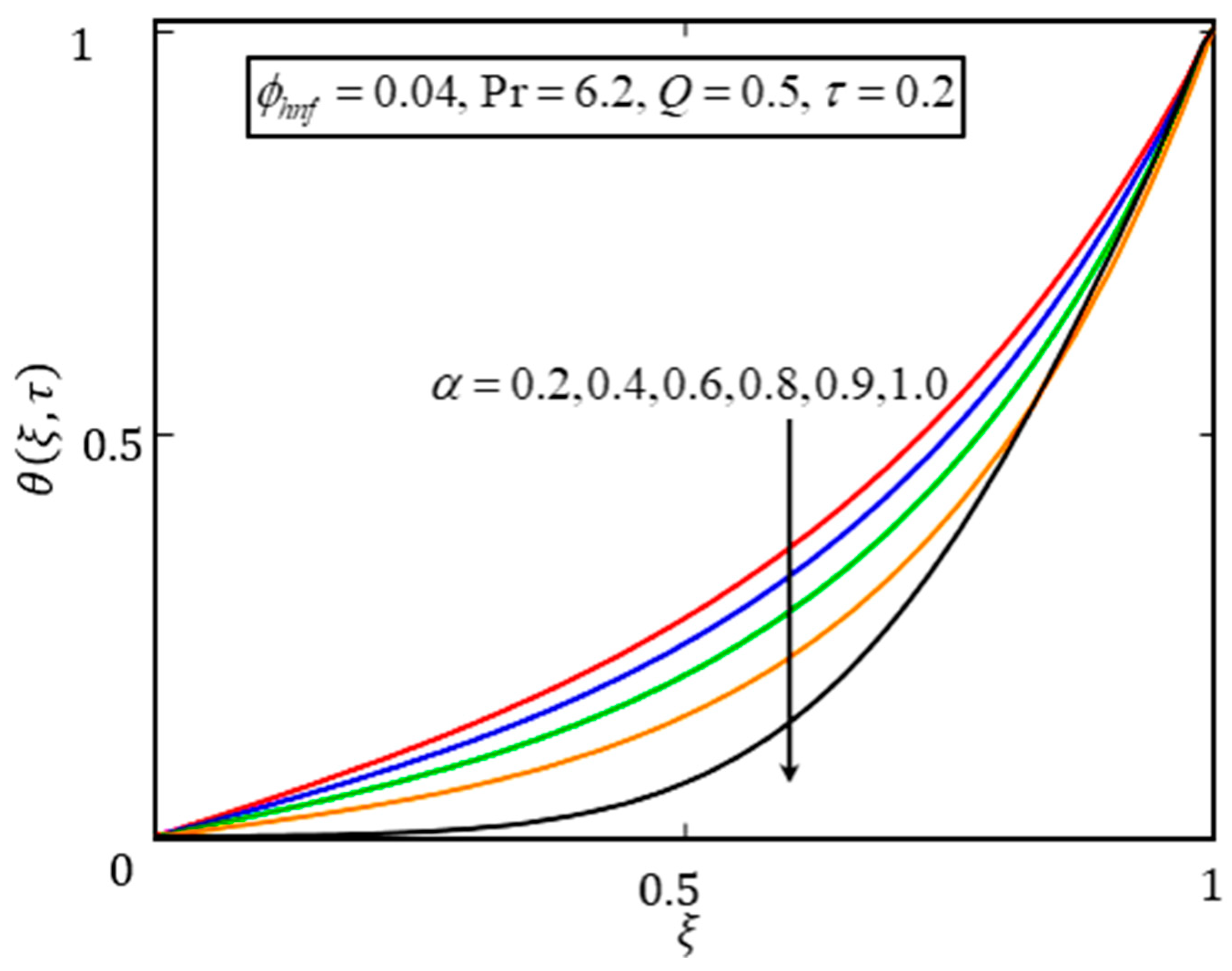
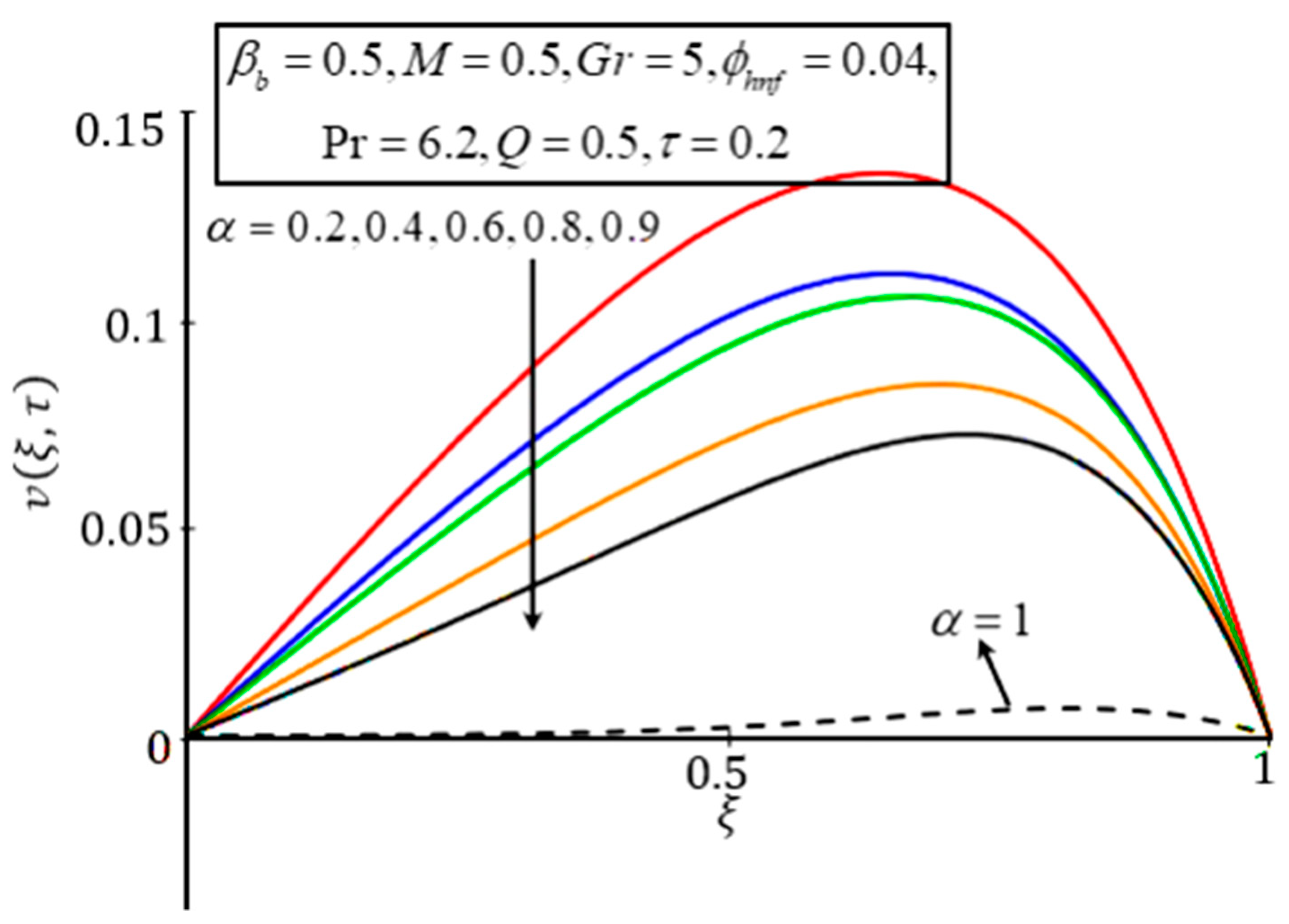
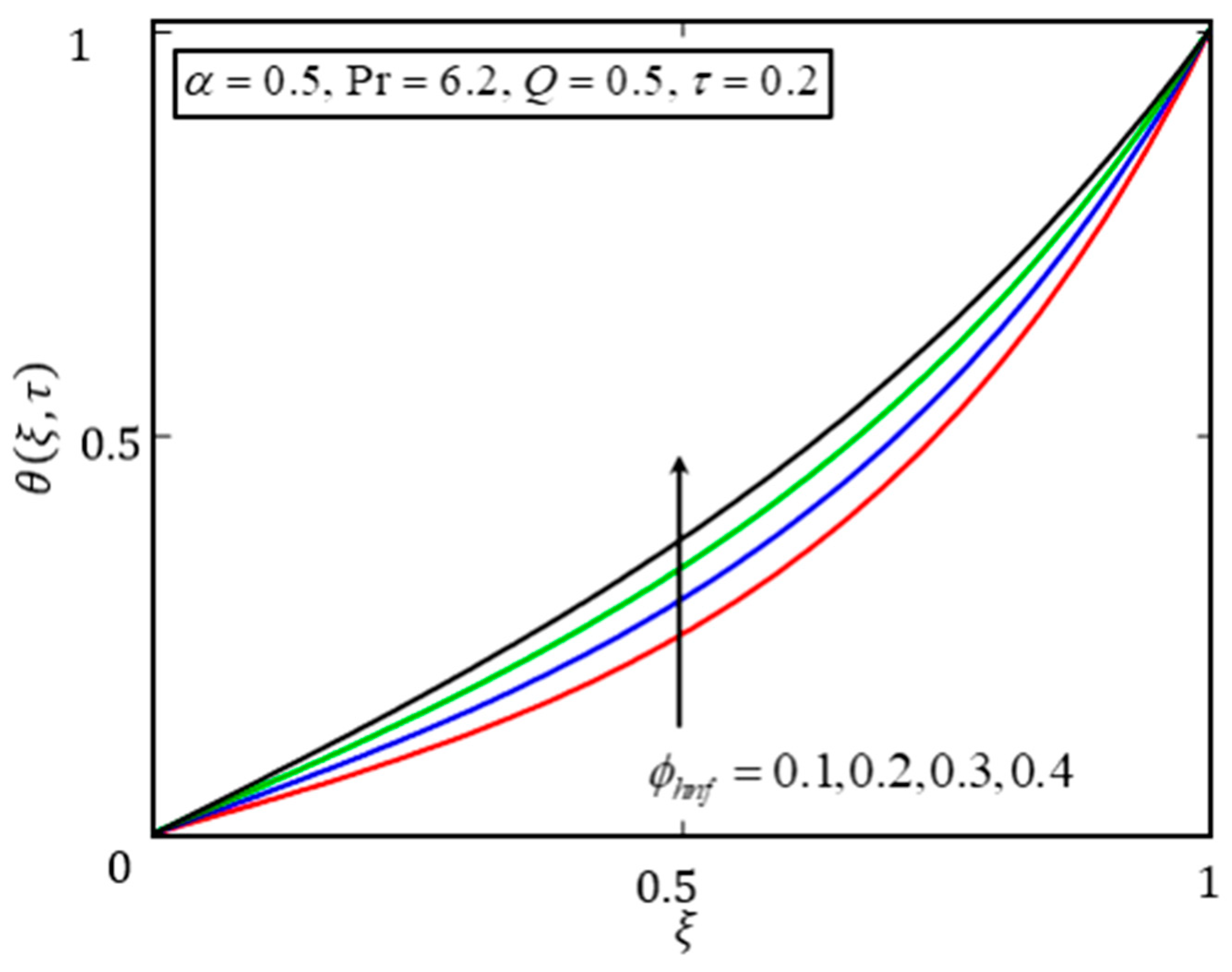
5. Results and Discussion

The $Ag-Ti{O}_2-H_{2}O$ hybrid nanofluid was characterized by fractional rheological analysis. The Brinkman type fluid model with buoyancy and magnetic body forces was considered with a partially coupled energy equation and heat generation. To analyze the rheological behavior of the hybrid nanofluid, the fractional model was solved via the Laplace transform technique. The fractional solutions of the velocity and temperature profiles in terms of CFFO are presented in numerous graphs and discussed. The effects of $\alpha$, ${\varphi }_{hnf}$, $Q$, ${\beta }_b$, $M$ and $Gr$ on velocity and temperature distributions are also explored.

The effect of $\alpha$ on the velocity and temperature profiles is displayed in Figure 2 and Figure 3. It may be seen that the velocity and temperature profiles caused significantly variation of $\alpha$. Furthermore, was observed that increasing values of $\alpha$ leads to a reduction in the velocity and temperature profiles due to a decrease in momentum and thermal and boundary layers. At $\alpha =1$, the thermal and momentum boundary layers were the thinnest. At this point, the temperature and velocity became minimum. This trend indicates that fractional results are more flexible and have a memory effect. Agreement could be established among theoretical and experimental data by setting the values of $\alpha$ in the manner established by Markis et al. [45] while studying Maxwell fluid. Azhar et al. [46] reported the same trend of the fractional parameter for a conventional nanofluid near a vertical plate via CFFO and integral transform.

Figure 4 and Figure 5 present the impact of ${\varphi }_{hnf}$ on the temperature and velocity profiles. The temperature profile shows an increasing trend with increasing values of ${\varphi }_{hnf}$. It is evident from Table 2 that larger values of ${\varphi }_{hnf}$ enhance the capability of hybrid nanofluid to absorb more heat. However, the effect of ${\varphi }_{hnf}$ on the velocity profile is the opposite. From Table 2, it can be observed that when ${\varphi }_{hnf}$ is increased, it leads to an increase in density and viscosity, and a decrease in velocity. The same trend for ${\varphi }_{hnf}$ was reported by Farooq et al. [21]. It must be remembered that this effect is true when the temperature of the fluid is between 0 °C and 180 °C.

A comparison of the temperature and velocity profiles for $H_{2}O$ (regular fluid), $Ti{O}_2-H_{2}O$ (nanofluid), $Ag-H_{2}O$ (nanofluid) and $Ag-Ti{O}_2-H_{2}O$ (hybrid nanofluid) is made in Figure 6 and Figure 7. As $Ag$ is a good conductor, the $Ag-H_{2}O$ nanofluid had the highest and water the lowest temperature profile among the fluids under consideration. The main aim here is to increase the heat transport capacity of the $Ti{O}_2-H_{2}O$ nonfluid, as $Ti{O}_2$ is a semiconductor. $Ag$ transfers free electrons to $Ti{O}_2$, and consequently, the thermal conductivity of $Ag-Ti{O}_2-H_{2}O$ improves the heat transfer. The heat transfer in $Ag-Ti{O}_2-H_{2}O$ is higher than those of $Ti{O}_2-H_{2}O$ and water. On the other hand, the density of the nanofluid is a dominant factor that plays a role in the velocity profile. The densities of the base fluid and nanoparticles are presented in Table 1. Based on the differences in densities, the velocity of $H_{2}O$ is highest, followed by $Ti{O}_2-H_{2}O$, $Ag-Ti{O}_2-H_{2}O$ and $Ag-H_{2}O$. In this case, the effective density dominates the effective thermal conductivity as a result of pure water showing high velocity. In other words, by adding nanoparticles to the base fluid, the resulting nanofluid and hybrid nanofluids become denser which decreases their velocity [45,46,47,48,49,50].

To study the impact of $Q$ on the temperature and velocity profiles, Figure 8 and Figure 9 were plotted. The trend of $Q$ is very straight forward. When $Q$ increases, the system produces more heat, due to which the temperature and velocity distributions increase. The effect of ${\beta }_b$ on the velocity profile is summarized in Figure 10. An increase in ${\beta }_b$ decreases the fluid velocity because of higher values of ${\beta }_b$ strengthening the drag forces, which tends to decrease the velocity profile. A similar effect was reported by Jan et al. [35].

The effect of $M$ is displayed in Figure 11; it indicates that the velocity decreases with a higher value of $M$. Greater values of $M$ relate to greater resistive type forces, called Lorentz forces, which are like drag forces. For this reason, the velocity was reduced. Figure 12 reveals the influence of $Gr$ on the velocity profile. It is seen that the velocity accelerated with higher $Gr$. The higher $Gr$ is connected to greater buoyancy forces which increase the natural convection; hence, the velocity increases in speed:

6. Conclusions

This article studied the rheological behavior of a $Ag-Ti{O}_2-H_{2}O$ hybrid nanofluid. The flow of the nanofluid was considered in a microchannel. The MHD and heat generation effects were also taken into consideration. The local flow model was converted to a fractional model using CFFO. The exact solutions were obtained using the Laplace transform method. The exact solutions for the temperature and velocity e profiles were simulated and presented in various graphs with a physical explanation. It was concluded that the temperature and velocity fields showed an increasing trend with increasing values of $Q$ and $Gr$. However, a decreasing trend was found for increasing values of $\alpha$, ${\beta }_b\mathrm{and}M$. In contrast, for ${\varphi }_{hnf}$, the temperature and velocity profiles showed the opposite behavior.

References

1. Usman, M.; Hamid, M.; Zubair, T.; Haq, R.U.; Wang, W. Cu-Al2O3/Water hybrid nanofluid through a permeable surface in the presence of nonlinear radiation and variable thermal conductivity via LSM. Int. J. Heat Mass Transf. 2018, 126, 1347–1356. [Google Scholar] [CrossRef]
2. Ellahi, R.; Hassan, M.; Zeeshan, A. Shape effects of spherical and nonspherical nanoparticles in mixed convection flow over a vertical stretching permeable sheet. Mech. Adv. Mater. Struct. 2017, 24, 1231–1238. [Google Scholar] [CrossRef]
3. Ellahi, R.; Hussain, F.; Ishtiaq, F.; Hussain, A. Peristaltic transport of Jeffrey fluid in a rectangular duct through a porous medium under the effect of partial slip: An application to upgrade industrial sieves/filters. Pramana 2019, 93, 34. [Google Scholar] [CrossRef]
4. Ellahi, R.; Raza, M.; Akbar, N.S. Study of peristaltic flow of nanofluid with entropy generation in a porous medium. J. Porous Media 2017, 20, 461–478. [Google Scholar] [CrossRef]
5. Ellahi, R.; Tariq, M.H.; Hassan, M.; Vafai, K. On boundary layer nano-ferroliquid flow under the influence of low oscillating stretchable rotating disk. J. Mol. Liq. 2017, 229, 339–345. [Google Scholar] [CrossRef]
6. Ellahi, R.; Zeeshan, A.; Hussain, F.; Abbas, T. Two-phase couette flow of couple stress fluid with temperature dependent viscosity thermally affected by magnetized moving surface. Symmetry 2019, 11, 647. [Google Scholar] [CrossRef] [Green Version]
7. Routbort, J.L.; Singh, D.; Chen, G. Heavy Vehicle Systems Optimization Merit Review and Peer Evaluation; Annual Report; Argonne National Laboratory: Chicago, IL, USA, 2006. [Google Scholar]
8. Lee, S.; Choi, S.-S.; Li, S.A.; Eastman, J.A. Measuring thermal conductivity of fluids containing oxide nanoparticles. J. Heat Transf. 1999, 121, 280–289. [Google Scholar] [CrossRef]
9. Mahian, O.; Kolsi, L.; Amani, M.; Estellé, P.; Ahmadi, G.; Kleinstreuer, C.; Marshall, J.S.; Siavashi, M.; Taylor, R.A.; Niazmand, H. Recent advances in modeling and simulation of nanofluid flows-part I: Fundamental and theory. Phys. Rep. 2018, 1–48. [Google Scholar] [CrossRef]
10. Mahian, O.; Kolsi, L.; Amani, M.; Estellé, P.; Ahmadi, G.; Kleinstreuer, C.; Marshall, J.S.; Taylor, R.A.; Abu-Nada, E.; Rashidi, S. Recent advances in modeling and simulation of nanofluid flows-part II: Applications. Phys. Rep. 2018. [Google Scholar] [CrossRef]
11. Vallejo, J.P.; Żyła, G.; Fernández-Seara, J.; Lugo, L. Rheological behaviour of functionalized graphene nanoplatelet nanofluids based on water and propylene glycol: Water mixtures. Int. Commun. Heat Mass Transf. 2018, 99, 43–53. [Google Scholar] [CrossRef]
12. Vallejo, J.P.; Żyła, G.; Fernández-Seara, J.; Lugo, L. Influence of Six Carbon-Based Nanomaterials on the Rheological Properties of Nanofluids. Nanomaterials 2019, 9, 146. [Google Scholar] [CrossRef] [PubMed] [Green Version]
13. Żyła, G.; Fal, J.; Bikić, S.; Wanic, M. Ethylene glycol based silicon nitride nanofluids: An experimental study on their thermophysical, electrical and optical properties. Phys. E Low Dimens. Syst. Nanostruct. 2018, 104, 82–90. [Google Scholar] [CrossRef]
14. Fal, J.; Mahian, O.; Żyła, G. Nanofluids in the Service of High Voltage Transformers: Breakdown Properties of Transformer Oils with Nanoparticles, a Review. Energies 2018, 11, 2942. [Google Scholar] [CrossRef] [Green Version]
15. Fal, J.; Żyła, G. Effect of Temperature and Mass Concentration of SiO2 Nanoparticles on Electrical Conductivity of Ethylene Glycol. Acta Phys. Pol. A 2017, 132, 155–157. [Google Scholar] [CrossRef]
16. Murshed, S.M.S.; Estellé, P. A state of the art review on viscosity of nanofluids. Renew. Sustain. Energy Rev. 2017, 76, 1134–1152. [Google Scholar] [CrossRef]
17. Estellé, P.; Cabaleiro, D.; Żyła, G.; Lugo, L.; Murshed, S.M.S. Current trends in surface tension and wetting behavior of nanofluids. Renew. Sustain. Energy Rev. 2018, 94, 931–944. [Google Scholar] [CrossRef]
18. Rashad, A.M.; Chamkha, A.J.; Ismael, M.A.; Salah, T. MHD Natural Convection in a Triangular Cavity filled with a Cu-Al2O3/Water Hybrid Nanofluid with Localized Heating from Below and Internal Heat Generation. J. Heat Transf. 2018, 7, 140. [Google Scholar]
19. Izadi, M.; Mohebbi, R.; Delouei, A.A.; Sajjadi, H. Natural convection of a Magnetizable hybrid nanofluid inside a porous enclosure subjected to two variable magnetic fields. Int. J. Mech. Sci. 2019, 151, 154–169. [Google Scholar] [CrossRef]
20. Shahsavar, A.; Moradi, M.; Bahiraei, M. Heat transfer and entropy generation optimization for flow of a non-Newtonian hybrid nanofluid containing coated CNT/Fe3O4 nanoparticles in a concentric annulus. J. Taiwan Inst. Chem. Eng. 2018, 84, 28–40. [Google Scholar] [CrossRef]
21. Farooq, U.; Afridi, M.; Qasim, M.; Lu, D. Transpiration and Viscous Dissipation Effects on Entropy Generation in Hybrid Nanofluid Flow over a Nonlinear Radially Stretching Disk. Entropy 2018, 20, 668. [Google Scholar] [CrossRef] [Green Version]
22. Caputo, M. Linear models of dissipation whose Q is almost frequency independent—II. Geophys. J. Int. 1967, 13, 529–539. [Google Scholar] [CrossRef]
23. Saqib, M.; Khan, I.; Shafie, S. New Direction of Atangana—Baleanu Fractional Derivative with Mittag-Leffler Kernel for Non-Newtonian Channel Flow. In Fractional Derivatives with Mittag-Leffler Kernel; Springer: Basel, Switzerland, 2019; pp. 253–268. [Google Scholar]
24. Metzler, R.; Klafter, J. The random walk’s guide to anomalous diffusion: A fractional dynamics approach. Phys. Rep. 2000, 339, 1–77. [Google Scholar] [CrossRef]
25. Caputo, M.; Fabrizio, M. A new definition of fractional derivative without singular kernel. Prog. Fract. Differ. Appl. 2015, 1, 1–13. [Google Scholar]
26. Ali, F.; Saqib, M.; Khan, I.; Sheikh, N.A. Application of Caputo-Fabrizio derivatives to MHD free convection flow of generalized Walters’-B fluid model. Eur. Phys. J. Plus 2016, 131, 377. [Google Scholar] [CrossRef]
27. Sheikh, N.A.; Ali, F.; Khan, I.; Saqib, M. A modern approach of Caputo—Fabrizio time-fractional derivative to MHD free convection flow of generalized second-grade fluid in a porous medium. Neural Comput. Appl. 2018, 30, 1865–1875. [Google Scholar] [CrossRef]
28. Zafar, A.A.; Fetecau, C. Flow over an infinite plate of a viscous fluid with non-integer order derivative without singular kernel. Alex. Eng. J. 2016, 55, 2789–2796. [Google Scholar] [CrossRef] [Green Version]
29. Hristov, J. Derivatives with non-singular kernels from the Caputo—Fabrizio definition and beyond: Appraising analysis with emphasis on diffusion models. Front. Fract. Calc. 2017, 1, 270–342. [Google Scholar]
30. Atangana, A.; Koca, I. On the new fractional derivative and application to nonlinear Baggs and Freedman model. J. Nonlinear Sci. Appl. 2016, 9, 5. [Google Scholar] [CrossRef] [Green Version]
31. Atangana, A.; Baleanu, D. New fractional derivatives with nonlocal and non-singular kernel: Theory and application to heat transfer model. Therm. Sci. 2016, 20, 763–769. [Google Scholar] [CrossRef] [Green Version]
32. Caputo, M.; Fabrizio, M. On the notion of fractional derivative and applications to the hysteresis phenomena. Meccanica 2017, 52, 3043–3052. [Google Scholar] [CrossRef]
33. Hristov, J.Y. Linear viscoelastic responses: The Prony decomposition naturally leads into the Caputo-Fabrizio fractional operator. Front. Phys. 2018, 6, 135. [Google Scholar] [CrossRef]
34. Tashtoush, B.; Magableh, A. Magnetic field effect on heat transfer and fluid flow characteristics of blood flow in multi-stenosis arteries. Heat Mass Transf. 2008, 44, 297–304. [Google Scholar] [CrossRef]
35. Jan, S.A.A.; Ali, F.; Sheikh, N.A.; Khan, I.; Saqib, M.; Gohar, M. Engine oil based generalized brinkman-type nano-liquid with molybdenum disulphide nanoparticles of spherical shape: Atangana-Baleanu fractional model. Numer. Methods Partial Differ. Equ. 2018, 34, 1472–1488. [Google Scholar] [CrossRef]
36. Aminossadati, S.M.; Ghasemi, B. Natural convection cooling of a localised heat source at the bottom of a nanofluid-filled enclosure. Eur. J. Mech. B Fluids 2009, 28, 630–640. [Google Scholar] [CrossRef]
37. Brinkman, H.C. The viscosity of concentrated suspensions and solutions. J. Chem. Phys. 1952, 20. [Google Scholar] [CrossRef]
38. Bourantas, G.C.; Loukopoulos, V.C. Modeling the natural convective flow of micropolar nanofluids. Int. J. Heat Mass Transf. 2014, 68, 35–41. [Google Scholar] [CrossRef]
39. Levin, M.L.; Miller, M.A. Maxwell a treatise on electricity and magnetism. Uspekhi Fiz. Nauk 1981, 135, 425–440. [Google Scholar] [CrossRef]
40. Maxwell, J.C. Electricity and Magnetism; Dover: New York, NY, USA, 1954. [Google Scholar]
41. Tiwari, R.K.; Das, M.K. Heat transfer augmentation in a two-sided lid-driven differentially heated square cavity utilizing nanofluids. Int. J. Heat Mass Transf. 2007, 50, 2002–2018. [Google Scholar] [CrossRef]
42. Saqib, M.; Khan, I.; Shafie, S.; Qushairi, A. Recent Advancment in Thermophysical Properties of Nanofluids and Hybrid Nanofluids: An Overview. City Univ. Int. J. Comput. Anal. 2019, 3, 16–25. [Google Scholar]
43. Hussain, S.; Ahmed, S.E.; Akbar, T. Entropy generation analysis in MHD mixed convection of hybrid nanofluid in an open cavity with a horizontal channel containing an adiabatic obstacle. Int. J. Heat Mass Transf. 2017, 114, 1054–1066. [Google Scholar] [CrossRef]
44. Saqib, M.; Khan, I.; Shafie, S. Application of fractional differential equations to heat transfer in hybrid nanofluid: Modeling and solution via integral transforms. Adv. Differ. Equ. 2019, 2019, 52. [Google Scholar] [CrossRef] [Green Version]
45. Makris, N.; Dargush, G.F.; Constantinou, M.C. Dynamic analysis of generalized viscoelastic fluids. J. Eng. Mech. 1993, 119, 1663–1679. [Google Scholar] [CrossRef]
46. Azhar, W.A.; Vieru, D.; Fetecau, C. Free convection flow of some fractional nanofluids over a moving vertical plate with uniform heat flux and heat source. Phys. Fluids 2017, 29, 082001. [Google Scholar] [CrossRef]
47. Safaei, M.R.; Ahmadi, G.; Goodarzi, M.S.; Safdari Shadloo, M.; Goshayeshi, H.R.; Dahari, M. Heat Transfer and Pressure Drop in Fully Developed Turbulent Flows of Graphene Nanoplatelets—Silver/Water Nanofluids. Fluids 2016, 1, 20. [Google Scholar] [CrossRef] [Green Version]
48. Abdollahzadeh Jamalabadi, M.Y.; Ghasemi, M.; Alamian, R.; Wongwises, S.; Afrand, M.; Shadloo, M.S. Modeling of Subcooled Flow Boiling with Nanoparticles under the Influence of a Magnetic Field. Symmetry 2019, 11, 1275. [Google Scholar] [CrossRef] [Green Version]
49. Irandoost Shahrestani, M.; Maleki, A.; Safdari Shadloo, M.; Tlili, I. Numerical Investigation of Forced Convective Heat Transfer and Performance Evaluation Criterion of Al2O3/Water Nanofluid Flow inside an Axisymmetric Microchannel. Symmetry 2020, 12, 120. [Google Scholar] [CrossRef] [Green Version]
50. Ellahi, R.; Hussain, F.; Abbas, S.A.; Sarafraz, M.M.; Goodarzi, M.; Safdari Shadloo, M. Study of two-phase newtonian nanofluid flow hybrid with hafnium particles under the effects of slip. Inventions 2020, 5, 6. [Google Scholar] [CrossRef] [Green Version]
Figure 1. Configuration of microchannel and coordinates system.
Symmetry 12 00663 g001
Figure 2. Plot of ξ for different values of α .
Symmetry 12 00663 g002
Figure 3. Velocity Plot of ξ for different values of α .
Symmetry 12 00663 g003
Figure 4. Temperature plot of ξ for different values of ϕ h n f .
Symmetry 12 00663 g004
Figure 5. Velocity plot of ξ for different values of ϕ h n f .
Symmetry 12 00663 g005
Figure 6. Temperature profile of ξ for different nanofluids.
Symmetry 12 00663 g006
Figure 7. Velocity profile of ξ for different nanofluids.
Symmetry 12 00663 g007
Figure 8. Plot of ξ for different values of Q .
Symmetry 12 00663 g008
Figure 9. Plot of ξ for different values of Q .
Symmetry 12 00663 g009
Figure 10. Plot of ξ for different values of β b .
Symmetry 12 00663 g010
Figure 11. Plot of ξ for different values of M .
Symmetry 12 00663 g011
Figure 12. Plot of ξ for different values of G r .
Symmetry 12 00663 g012