Abstract
The process of machine learning is to find parameters that minimize the cost function constructed by learning the data. This is called optimization and the parameters at that time are called the optimal parameters in neural networks. In the process of finding the optimization, there were attempts to solve the symmetric optimization or initialize the parameters symmetrically. Furthermore, in order to obtain the optimal parameters, the existing methods have used methods in which the learning rate is decreased over the iteration time or is changed according to a certain ratio. These methods are a monotonically decreasing method at a constant rate according to the iteration time. Our idea is to make the learning rate changeable unlike the monotonically decreasing method. We introduce a method to find the optimal parameters which adaptively changes the learning rate according to the value of the cost function. Therefore, when the cost function is optimized, the learning is complete and the optimal parameters are obtained. This paper proves that the method ensures convergence to the optimal parameters. This means that our method achieves a minimum of the cost function (or effective learning). Numerical experiments demonstrate that learning is good effective when using the proposed learning rate schedule in various situations.
1. Introduction
Machine learning is carried out by using a cost function to determine how accurately a model learns from data and determining the parameters that minimize this cost function. The process of changing these parameters, in order to find the optimal set, is called learning. We define a cost function to check that the learning is successful: the lower the value of the cost function, the better the learning. The cost function is also used in the learning process. Therefore, the cost function is selected and used for learning, according to the training data [1,2]. In the learning process, a gradient-based method is usually used to reduce the gradient of the cost function [3,4,5,6,7,8]. However, with larger sets of training data and more complex training models, the cost function many have many local minima, and the simple gradient descent method fails at a local minimum because the gradient vanishes at this point. To solve this problem, some gradient-based methods where learning occurs even when the gradient is zero have been introduced, such as momentum-based methods. In these methods, the rate of change of the cost function is continuously added to the ratio of an appropriate variable. Even if the rate of change of the cost function becomes zero, the learning is continued by the value of the rate of change of the previously added cost function [9]. It is not known whether the situation where learning stopped (parameters change no longer occurs) is the optimal situation for the cost function. One of the important factors in optimization using gradient-based methods is a hyperparameter called the learning rate (or step-size). If the norm of the gradient is large, the learning will not work well. If the norm of the gradient is small, the learning will be too slow [10]. In order to solve this problem, learning rate schedules have been introduced. The usual learning rate schedule is a constant that is multiplied by the gradient in the learning process. However, since the learning rate set initially is a constant, the gradient may not be scaled during learning. To solve this problem, other methods have been developed to schedule the learning rate, such as step-based and time-based methods, where it is not a constant but a function which becomes smaller as learning progresses [11,12,13,14]. Furthermore, adaptive optimization methods with the effect of changing the learning rate have been developed, such as Adagrad and RMSProp [15,16,17,18,19,20,21,22]. Currently, adaptive optimization methods and adaptive learning rate schedules are used in combination. However, the learning rate schedules used currently only decrease as learning progresses, which may be a factor in causing the learning to not proceed further at a local minimum [23,24,25,26,27]. In this paper, we introduce a method to increase the learning rate, depending on the situation, rather than just decreasing as the learning progresses. For our numerical experiments, we chose the most basic Gradient Descent (GD) method, the momentum method, and the most widely known Adam method as the basic methodologies for comparison. We computed the change of numerical value according to each methodology and each learning rate schedule.
This paper is organized as follows. Section 2 explains the existing learning methods. This section discusses the basic GD method, the momentum method, learning rate methods, and the Adam method, which is a combination of them. Finally, descriptions of some more advanced methods based on Adam (i.e., Adagrad, RMSProp, and AdaDelta) are given. Section 3 explains our method and proves its convergence. Section 4 demonstrates that our proposed method is superior to the existing methods through various numerical experiments. The numerical experiments in this section consist of Weber’s function experiments, to test for changes in multidimensional space and local minima, binary classification experiments, and classification experiments with several classes [28].
2. Machine Learning Method
As explained in the previous section, machine learning is achieved through optimization of the cost function. Generally, the learning data are divided into input data and output data. Here, we denote the input data by x and the output data by y. Assuming that there are l training data, we conform the following data: . That is, when the value of is entered, the value of is expected. The function is created by an artificial neural network (ANN). The most basic is constructed as follows.
where is called an activation function, where a non-linear function is used. We want the obtained from an artificial neural network to have the same value as y, and we can define the cost function as
The process of finding the parameters which minimize this cost function C is machine learning. More detailed information can be found in [20].
2.1. Direction Method
This section introduces ways to minimize the cost function satisfying that
Machine learning is completed by determining the parameters that satisfy the Equation (4) [12,25,27,28].
2.1.1. Gradient Descent Method
GD is the simplest of the gradient-based methods. This method is based on the fixed iteration method in mathematics. The update rule of this method is as follows:
where is a (constant) learning rate [12,25,27,28].
2.1.2. Momentum Method
Gradient-based optimization methods were designed under the assumption that the cost function is convex [10]. However, in general, the cost function is not a convex function. This causes problems with poor learning at local minima. The momentum method was introduced to solve this problem. The update rule of this method is as follows:
where is a constant [9].
2.2. Learning Rate Schedule
In gradient-based methods, one problem is that the parameters are not optimized when the size of the gradient is large. To solve this problem, we multiply the gradient by a small constant (called the learning rate) in the parameter update rule. However, in order to improve learning efficiency, methods for changing the value at each step, instead of using a constant learning rate, are used. We will introduce some learning rate schedule methods below.
2.2.1. Time-Based Learning Rate Schedule
The time-based learning rate schedule is the simplest learning rate schedule change rule. It has the form of a rational function whose denominator is a linear function:
where n is the iteration step, is the learning rate at the step, and d is the decay rate. This update rule changes the learning rate as learning progresses, reducing the denominator. As n starts at zero, 1 is added to prevent the denominator from being zero [11].
2.2.2. Step-Based Learning Rate Schedule
The update rule in the time-based learning rate schedule is a simple rational function. To increase its efficiency, update rules have been developed using exponential functions, as follows:
where n is the iteration step, is the initial learning rate, d is the decay rate (which is set to a real number between 0 and 1), and r is the drop rate. Therefore, the step-based learning rate always decreases [13].
2.2.3. Exponential-Based Learning Rate Schedule
The step-based learning rate schedule is discrete, as it uses the floor function in its update rule. The exponential-based schedule is made continuous by using an exponential function without a floor function, as follows:
where n is the iteration step, is the initial learning rate, and d is the decay rate [14]. A pseudocode version of this schedule is given in Algorithm 1.
| Algorithm 1: Pseudocode of exponential-based learning rate schedule. |
| : Initialize learning rate |
| d: Decay rate |
| (Initialize time step) |
2.3. Adaptive Optimization Methods
Gradient-based methods, such as those introduced in Section 2.1, only use a constant learning rate. To learn well in non-convex situations, methods such as the momentum method have been introduced, however, in order to increase the efficiency of learning, adaptive optimization methods have been developed. These methods have the effect of changing the learning rate in the optimization step. This section introduces some adaptive optimization methods.
2.3.1. Adaptive Gradient (Adagrad)
The Adagrad method is an adaptive method which changes the learning rate by dividing the learning rate by the -norm of the gradient at each step. In the denominator, the square of the gradient at each step is added; therefore, as the learning progresses, the denominator becomes larger. The update rule of this method is as follows:
where is the learning rate and is the gradient at the step. In this method, the learning rate in the step is / [15].
2.3.2. Root Mean Square Propagation (RMSProp)
RMSProp is an adaptive method which changes the learning rate in each step by dividing the learning rate by the square root of the exponential moving average of the square of the gradient. The update rule of this method is as follows:
where is the learning rate, is the gradient at the step, and is the exponential moving average (EMA) coefficient. In this method, the learning rate in the step is is / [16].
2.3.3. Adaptive Moment Estimation (Adam)
The Adam method was designed by combining Adagrad and RMSProp. It is the most widely used gradient-based method. The update rule of the Adam method is as follows:
where
, and . The Adam method calculates the EMA for each of the gradients and the squares of the gradient and uses their ratios to adjust the learning rate [18,19,20]. The pseudocode version of this method is given in Algorithm 2.
| Algorithm 2: Pseudocode of Adam method. |
| : Learning rate |
| : Exponential decay rates for the moment estimates |
| : Cost function with parameters w |
| : Initial parameter vector |
| (Initialize timestep) |
| not converged |
| (Resulting parameters) |
3. The Proposed Method
The various algorithms introduced in Section 2 either do not change (constant) or only decrease the learning rate. These cannot be avoided when the parameter reaches a local minimum. Therefore, we introduce a new learning rate schedule using cost functions. The pseudocode version of proposed method is given in Algorithm 3.
| Algorithm 3: Pseudocode of cost-based learning rate schedule. |
| : Initialize learning rate |
| : Cost function with parameters w |
| (Initialize time step) |
The cost-based learning rate schedule can be used in conjunction with other (adaptive) optimization methods. This paper proves its convergence when used with the Adam method. Equation (15) is as follows:
As and are 0.9 and 0.999, respectively, if i is large enough, then can be regarded as 1 (see Appendix A.1 for details). Therefore, our proposed method is obtained by the following equation:
where
Here, we change the learning rate from the existing to the function , such that the change of the cost function is reflected in optimization. From Equation (20), we can obtain the sequence . See Appendix A.2 for the process of obtaining Equation (22). In this paper, we will show that our sequence converges and that the limit value of the sequence satisfies the minimum value of the cost function.
Lemma 1.
The relationship between and is
Proof.
More details can be found in [20]. □
The Equation (20) is changed as
by Lemma 1 (the relationship between and ). In this equation, is intended to avoid the denominator going to zero and can be regarded as not present in the calculation. In order for the value of the right part of the Equation (24) to converge to zero, the value of should be smaller than 1 and the sequence converges to zero. Therefore, we must show that the cost function goes to zero under the condition of the sequence which we have defined [20].
Theorem 1.
Judgement on whether or not machine learning is well constructed depends on how small the value of the cost function is. Therefore, it is important to find the parameter whose cost function approaches zero. Evaluated at the parameter defined by our proposed method, the cost function is going to zero.
Proof.
In Theorem 1, it is possible that is less than 1. Therefore, in the following Lemma, we explain in more detail why is less than 1.
Lemma 2.
The δ defined in Theorem 1 is less than 1.
Proof.
First of all, i is assumed to be a number such that is sufficiently large. Under the condition of sufficiently small , the equation
can be divided into two parts, and can be computed as
and
The Equation (32) is obtained by an easy calculation. We must show that Equation (33) is less than 1. Under the assumption of this Lemma 2 and by the definition of , we get as and the sign does not change dramatically as is a continuous function. Therefore, we have . By Equation (33), we get
If , then there is or such that . Therefore, . Equation (33) is a small value, less than 1. By this process, we can set as a small constant and obtain the following result: . □
4. Numerical Tests
In this section, we detail the results of various numerical experiments. In each experiment, we compare the results of our proposed method with the numerical results of GD, momentum, and Adam with various learning rates. For the types of learning rates, we apply the constant, time-based, step-based, exponetial-based, and cost-based schedules described above.
4.1. Two-Variable Function Test Using Weber’s Function
In this section, we look at how the parameters change (according to how we compare them) using a two-variable function, Weber’s function. Weber’s function is
where is integer, = in such that , , and is a vector in [28].
4.1.1. Case 1: Weber’s Function with Three Terms Added
In this case, we used Weber’s function with the following variables as the cost function: , , , , and . This Weber’s function has a global minimum at .
In this experiment, the initial values were and . Figure 1 shows the given Weber’s function under these initial conditions. In Figure 1, the red point is its global minimum in . Figure 2 visualizes the change of parameters, according to the optimization methods and the learning rates introduced in this paper. In Figure 2a, the GD method was used and the results of the changes in the learning rate are visualized. In Figure 2b, the momentum method was used and the results of the changes in the learning rate are visualized. In Figure 2c, the Adam method was used and the results of the changes in the learning rate are visualized. In particular, we stopped learning before reaching the global minimum, in order to compare the convergence rates of each method. In this experiment, there were no local minima and all the methods converged well to the global minimum. In this experiment, our cost-based learning rate schedule combined with the optimization methods showed the fastest convergence speed.
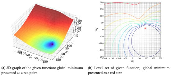
Figure 1.
Weber’s function for given μ and ν.
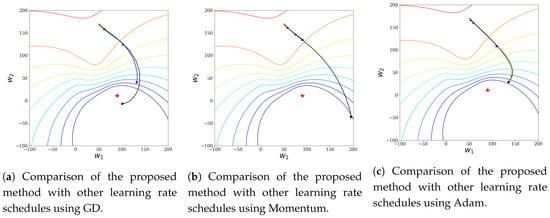
Figure 2.
Comparing methods with initial point (50, 170) and initial learning rate 5 × 10². The blue line, the red line, the green line, the yellow line, and the black line represent the constant learning rate schedule, the time-based learning rate schedule, the step-based learning rate schedule, the exponential-based learning rate schedule, and the cost-based learning rate schedule, respectively.
4.1.2. Case 2: Weber’s Function with Four Terms Added
In this case, we used the Weber’s function with the following variables as the cost function: , , , , , and . This Weber’s function had a local minimum at and a global minimum at . In Figure 3, the global minimum is represented by a red dot and the local minimum is represented by a blue dot. In this experiment, we wanted to see that each parameter produced by the learning rate constantly changed beyond the local minimum.
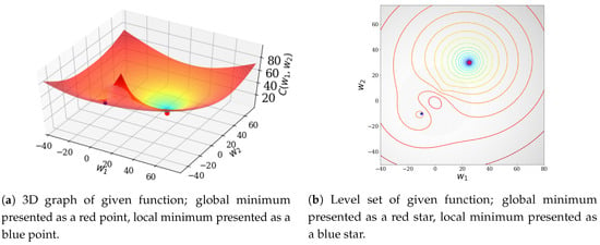
Figure 3.
Weber’s function for given μ and ν.
The initial values were and . Figure 4 visualizes the change of parameters according to the optimization methods and the learning rates introduced in this paper. In Figure 4a, the GD method was used and the results of the changes in the learning rate are visualized. In Figure 4b, the momentum method was used and the results of the changes in the learning rate are visualized. In Figure 4c, the Adam method was used and the results of the changes in the learning rate are visualized. In all optimization methods, we can see that only the cost-based learning rate schedule caused convergence beyond the local minimum to the value of the global minimum.
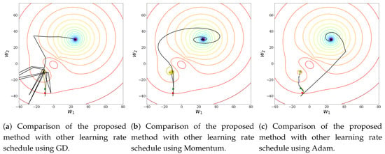
Figure 4.
Comparing methods with initial point (−10, −40)
and initial learning rate 5 × 10⁻¹. The blue line, the red line, the green line, the yellow line, and the black line represent the Constant learning rate schedule, the time-based learning rate schedule, the step-based learning rate schedule, the exponential-based learning rate schedule, and the cost-based learning rate schedule, respectively.
4.2. Binary Classification with Multilayer Perceptron (MLP)
In this section, a Binary Classification Problem (BCP) was implemented for each method using a MLP model. The BCP was based on a size image data set with ∘ and × draw. Figure 5 shows some images from the data set used in this experiment.

Figure 5.
Examples of data set used in this experiment.
The experiment was based on the Adam method in a six-layer MLP model, with different learning rate methods. The initial learning rate was set as and the number of iterations was 300.
Figure 6a shows the change in cost for each learning rate schedule during learning. Figure 6b shows the change in accuracy with each learning rate schedule during learning. As shown in Figure 6a, all methods quickly reduced cost (except for the constant learning rate). Unfortunately, the cost-based learning rate schedule had a high cost when learning; however, it was superior to other methods in terms of accuracy, as shown in Figure 6b.

Figure 6.
Result of binary classification with multilayer perceptron (MLP).
4.3. MNIST with MLP
In the next experiment, the MLP was used to solve a multi-classification problem using the MNIST data set, in order to verify the performance of each learning rate schedule. The images in the MNIST data set are grayscale numbered images (from 0 to 9) of size . The experiment was based on the Adam method in a five-layer MLP model with each learning rate schedule. The initial learning rate was set as and the number of iterations was 1000.
Figure 7a shows the change in cost for each learning rate schedule during learning. Figure 7b shows the change in accuracy with each learning rate schedule during learning. The cost and accuracy were not much different from the results in the previous section; the cost-based learning rate schedule was the fastest and had the highest accuracy.
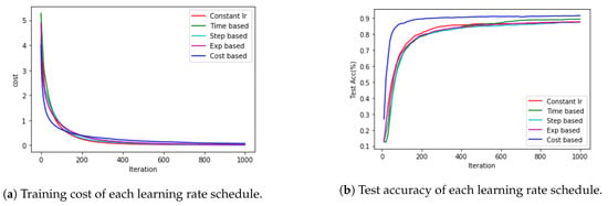
Figure 7.
Result of multi-classification with MLP.
4.4. MNIST with Convolutional Neural Network (CNN)
In this experiment, we sought to confirm that the proposed method has good performance when used in a deep learning framework. The performance of each method was measured using a Convolutional Neural Network (CNN) model for multi-class classification problems using the MNIST data set (the same as in Section 4.3). In this experiment, a CNN model with a first convolution filter of size , a second convolution filter of size , and a hidden layer of size 512 were used. In addition, the batch size was 64 and 50% dropout was used. The results are shown in Figure 8.
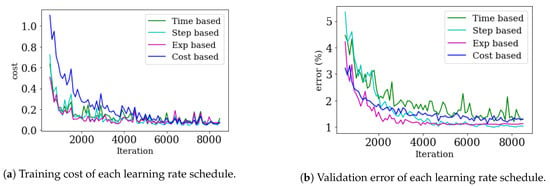
Figure 8.
Result of multi-classification with Convolutional Neural Network (CNN).
Figure 8a shows the change in cost for each learning rate schedule during learning. Figure 8b shows the change in validation error with each learning rate schedule during learning. It can be seen that all methods had no underfitting, due to the low training cost, and no overfitting, due to low validation error. Figure 8a shows that, at a given setting, the cost did not become relatively small, even though learning was progressing well. However, as the cost-based learning rate schedule is proportional to the cost, the learning rate is determined by the scale of the cost function when learning. Therefore, in this experiment, the cost-based learning rate schedule was slow; however, this can be solved (to some extent) by multiplying the cost function by a small constant. In this case, it was seen that the cost-based learning rate schedule was sensitive to the initial values of the cost function and the parameters.
5. Conclusions
This paper explains how the degree of learning varies with the learning rate in ANN-based machine learning. In particular, in general machine learning, local minima can cause problems in learning. In order to solve this problems, the existing methods used a monotonically decreasing learning rate at a constant rate according to the iteration time. However, these methods often lead to unexpected results that the cost function constructed by learning data is not approaching zero. In this paper, the machine learning methods worked well by use of our proposed learning rate schedule, which changes the learning rate appropriately.
By utilizing the value of the cost function in determining the change in the learning rate, we have the effect of stopping learning only at the global minimum of the cost function. The global minimum means that the cost we define is zero. Through our proposed method, the cost function converges to zero and in particular, it shows outstanding results in terms of learning accuracy. Our method has a characteristic that the learning rate is adaptive, and in particular, it has the advantage that it can be applied to existing learning methods by simply change the formula. The shortcoming of our method is if the cost of the initial parameters is high then the parameters do not learn well. However, this can be solved by multiplying the cost function by a constant smaller than 1.
Author Contributions
Conceptualization, D.Y. and S.J.; Data curation, S.J.; Formal analysis, D.Y.; Funding acquisition, D.Y.; Investigation, J.P.; Methodology, D.Y.; Project administration, D.Y.; Resources, J.P.; Software, S.J.; Supervision, J.P.; Validation, S.J.; Visualization, S.J.; Writing—original draft, J.P. and D.Y.; Writing—review & editing, J.P. and S.J. All authors have read and agreed to the published version of the manuscript.
Funding
This work was supported by the basic science research program through the National Research Foundation of Korea (NRF) funded by the Ministry of Education, Science and Technology (grant number NRF-2017R1E1A1A03070311).
Acknowledgments
We sincerely thank anonymous reviewers whose suggestions helped improve and clarify this manuscript greatly.
Conflicts of Interest
The authors declare no conflict of interest.
Appendix A
Appendix A.1
From Equation (17), we obtain following equation
where and are constant values between 0 and 1. In general, and use 0.9 and 0.999 respectively. This implies that for all . Thus,
Appendix A.2
References
- Bishop, C.M.; Wheeler, T. Pattern Recognition and Machine Learning; Springer: Berlin/Heidelberg, Germany, 2006. [Google Scholar]
- Hinton, G.E.; Srivastava, N.; Krizhevsky, A.; Sutskever, I.; Salakhutdinov, R.R. Improving neural networks by preventing co-adaptation of feature detectors. arXiv 2012, arXiv:1207.0580. [Google Scholar]
- Goodfellow, I.; Bengio, Y.; Courville, A. Deep Learning; The MIT Press Cambridge: London, UK, 2016. [Google Scholar]
- Dean, J.; Corrado, G.; Monga, R.; Chen, K.; Devin, M.; Le, Q.; Mao, M.; Ranzato, M.; Senior, A.; Tucker, P.; et al. Large scale distributed deep networks. In Proceedings of the 25th International Conference on Neural Information Processing Systems—NIPS 2012, Lake Tahoe, NV, USA, 3–6 December 2012; pp. 1223–1231. [Google Scholar]
- Amari, S. Natural gradient works efficiently in learning. Neural Comput. 1998, 10, 251–276. [Google Scholar] [CrossRef]
- Hinton, G.; Deng, L.; Yu, D.; Dahl, G.E.; Mohamed, A.; Jaitly, N.; Senior, A.; Vanhoucke, V.; Nguyen, P.; Sainath, T.N. Deep neural networks for acoustic modeling in speech recognition: The shared views of four research groups. Signal Process. Mag. 2012, 29, 82–97. [Google Scholar] [CrossRef]
- Krizhevsky, A.; Sutskever, I.; Hinton, G.E. Imagenet classification with deep convolutional neural networks. In Proceedings of the Neural Information Processing Systems–NIPS 2012, Lake Tahoe, NV, USA, 3–6 December 2012; pp. 1097–1105. [Google Scholar]
- Pascanu, R.; Bengio, Y. Revisiting natural gradient for deep networks. arXiv 2013, arXiv:1301.3584. [Google Scholar]
- Sutskever, I.; Martens, J.; Dahl, G.; Hinton, G.E. On the importance of initialization and momentum in deep learning. In Proceedings of the 30th International Conference on Machine Learning—ICML 2013, Atlanta, GA, USA, 16–21 June 2013; pp. 1139–1147. [Google Scholar]
- Forst, W.; Hoffmann, D. Optimization—Theory and Practice; Springer: Berlin/Heidelberg, Germany, 2010. [Google Scholar]
- Nesterov, Y. Introductory Lectures on Convex Optimization: A Basic Course; Springer: Berlin/Heidelberg, Germany, 2004. [Google Scholar]
- Bengio, Y. Practical recommendations for gradient-based training of deep architectures. arXiv 2012, arXiv:1206.5533. [Google Scholar]
- Ge, R.; Kakade, S.M.; Kidambi, R.; Netrapalli, P. The Step Decay Schedule: A Near Optimal, Geometrically Decaying Learning Rate Procedure For Least Squares. arXiv 2019, arXiv:1904.12838. [Google Scholar]
- Li, Z.; Arora, S. An Exponential Learning Rate Schedule for Deep Learning. arXiv 2019, arXiv:1910.07454. [Google Scholar]
- Duchi, J.; Hazan, E.; Singer, Y. Adaptive subgradient methods for online learning and stochastic optimization. J. Mach. Learn. Res. 2011, 12, 2121–2159. [Google Scholar]
- Tieleman, T.; Hinton, G.E. Lecture 6.5—RMSProp, COURSERA: Neural Networks for Machine Learning; Technical Report; University of Toronto: Toronto, ON, Canada, 2012. [Google Scholar]
- Zeiler, M.D. Adadelta: An adaptive learning rate method. arXiv 2012, arXiv:1212.5701. [Google Scholar]
- Kingma, D.P.; Ba, J. ADAM: A method for stochastic optimization. In Proceedings of the 3rd International Conference for Learning Representations—ICLR 2015, San Diego, CA, USA, 7–9 May 2015. [Google Scholar]
- Reddi, S.J.; Kale, S.; Kumar, S. On the Convergence of ADAM and Beyond. arXiv 2019, arXiv:1904.09237. [Google Scholar]
- Yi, D.; Ahn, J.; Ji, S. An Effective Optimization Method for Machine Learning Based on ADAM. Appl. Sci. 2020, 10, 1073. [Google Scholar] [CrossRef]
- Kochenderfer, M.; Wheeler, T. Algorithms for Optimization; The MIT Press Cambridge: London, UK, 2019. [Google Scholar]
- Bottou, L.; Curtis, F.E.; Nocedal, J. Optimization Methods for Large-Scale Machine Learning. SIAM Rev. 2018, 60, 223–311. [Google Scholar] [CrossRef]
- Roux, N.L.; Fitzgibbon, A.W. A fast natural newton method. In Proceedings of the 27th International Conference on Machine Learning—ICML 2010, Haifa, Israel, 21–24 June 2010; pp. 623–630. [Google Scholar]
- Sohl-Dickstein, J.; Poole, B.; Ganguli, S. Fast large-scale optimization by unifying stochastic gradient and quasi-newton methods. In Proceedings of the 31st International Conference on Machine Learning—ICML 2014, Beijing, China, 21–24 June 2014; pp. 604–612. [Google Scholar]
- Rumelhart, D.E.; Hinton, G.E.; Williams, R.J. Learning representations by back-propagating errors. Nature 1986, 323, 533–536. [Google Scholar] [CrossRef]
- Becker, S.; LeCun, Y. Improving the Convergence of Back-Propagation Learning with Second Order Methods; Technical Report; Department of Computer Science, University of Toronto: Toronto, ON, Canada, 1988. [Google Scholar]
- Kelley, C.T. Iterative methods for linear and nonlinear equations. In Frontiers in Applied Mathematics; SIAM: Philadelphia, PA, USA, 1995. [Google Scholar]
- Kelley, C.T. Iterative Methods for Optimization. In Frontiers in Applied Mathematics; SIAM: Philadelphia, PA, USA, 1999. [Google Scholar]
© 2020 by the authors. Licensee MDPI, Basel, Switzerland. This article is an open access article distributed under the terms and conditions of the Creative Commons Attribution (CC BY) license (http://creativecommons.org/licenses/by/4.0/).