Abstract
The hidden danger is the direct cause of coal mine accidents, and the number of hidden dangers in a certain area not only reflects the current safety situation, but also determines the development trend of safety production in this area to a large extent. By analyzing the formation and development law of the hidden dangers and hidden danger accident-induced mechanism in coal mines, it is concluded that there are some objective laws in the process of occurrence, development, weakening, and even stabilization of hidden dangers in a certain area. The development of the number of hidden dangers for a coal mine generally presents the law of similar normal distribution curve, with a certain degree of partial symmetry. Many years of hidden danger elimination in coal mines will accumulate large-scale hidden danger data. In this paper, by using the average value of hidden danger quantity in consecutive months to weaken the oscillation of hidden danger quantity sequence, and combining with gray model (1,1) and the neural network of extreme learning machine, and employing big data of hidden dangers available, a hidden danger quantity prediction model based on the gray neural network was established, and the experimental analysis and verification carried out. The results show that the model can achieve good prediction effect on the number of hidden dangers in a coal mine, which not only reflects the complex gray system behavior of hidden dangers of a coal mine, but also can predict dynamically. The safety management efficiency and emergency capacity of the coal mine enterprise will be greatly improved.
1. Introduction
Identification and control of hidden dangers is an effective way to prevent and control accidents in a coal mine [1,2]. The coal mines across China have established hidden danger identification system, and made hidden danger identification daily work. Such hidden dangers identified are enormous. According to statistics, the industrial and mining enterprises in 2013 alone had identified five million hidden dangers [3]. As coal mines intensify their efforts in work safety, the quantity of hidden dangers to be identified is ever-increasing, and big data has come into existence. However, after its inspection of the coal mines across China, the State Administration of Work Safety pointed out that identification and elimination was far below expectation, given that underreporting and false reporting were common, and the safety situation in the coal mines is still severe [4,5].
Research on the hidden dangers of coal mines presently focuses on statistical analysis on the quantity and features of the hidden dangers in different months or varieties. Regarding hidden dangers data extraction in the literature, [6] used the association rule and analyzed the rule of association of the responsible department for hidden dangers, hidden danger variety, hidden danger grade, and hidden danger scene. In [7], they applied 5W1H analysis approach and transformed loopholes into eight dimensions, including hidden danger time and space, and used the log-linear model to dig the relationship among the dimensions. In [8], they managed to predict the hidden danger quantity by the least square method and extreme learning machine. The purpose and essence of all these studies make use of big data to predict the features of hidden dangers to allow coal mine managers to make good preparations. Qualitative or quantitative research of those hidden dangers is of some applicational value, but prediction precision is not high and the operability is not strong. The hidden dangers largely determine the safety situation of a coal mine, and they play a decisive role in work safety.
Any accident is the result of the interaction of hidden dangers in time and in space. Hidden dangers cover four aspects: human, machine, environment, and management. The quantity of hidden dangers in a system shows a nonlinear relationship with influential factor, and is hard to be predicted by traditional classical mathematical models due to its randomness and volatility [9]. Hidden dangers are the result of the interaction of all risk factors in a system, and the hidden danger quantity features gray and uncertainty [10,11]. The gray prediction model is characterized by simple computation and only a few samples. Hence, prediction of hidden danger quantity can be considered as a gray system to be predicted. According to the characteristics of the gray system, it can be known that gray prediction is suitable for exponential growth. Therefore, prediction precision is yet to be improved. However, neural network is a nonlinear, self-adaptable system, and is fault-tolerant, but needs more samples and complex computation [12,13,14,15].
In order to further utilize the existing big data of hidden dangers and adopt scientific data processing algorithms to predict the number of hidden dangers in different areas of the coal mine and improve the shortcomings of the existing models, this paper combines the advantages of gray prediction and neural networks. We predict and then use the neural network to correct the residuals of the gray prediction model, which improves the accuracy and practicability of the model, and is of great significance for improving the level of coal mine safety production management.
2. Methodology
2.1. Principle of Hidden Danger Quantity Prediction
Hidden dangers represent unsafe human behavior, unsafe condition of the environment, unsafe condition of equipment, or defective management during work activity [16]. They evolved from hazards, which interact and eventually trigger accidents, as illustrated in Figure 1 [16,17]. If a workplace is considered as a system, each of its components is in continuous motion. The hidden dangers in the system are the middle status of motion, and accidents are the worst results of motion. Occurrence of accidents will produce new or secondary hidden dangers. The quantity of the hidden dangers in the system are the result of mutual restriction and interaction between the status and quantity at the previous moment and hidden danger identification and control capability. Hidden danger development has its objective regularity. A hidden danger cannot appear or disappear out of thin air. Its status value at any time is related to the status value at a previous time or previous timeframe. The majority of hidden dangers in a system do not appear alone, rather, they are induced by the available hidden dangers or the resulting accidents. Hence, the quantity of hidden dangers, on the one hand, reflects the level of hidden danger identification and control capability in the previous timeframe, and on the other hand, determines the development trend of hidden danger in future time. Although, due to the error of artificial examination, the hidden danger quantity identified every month shows a volatility. On the whole, the hidden danger quantity will increase, decrease, or stabilize along with the hidden danger control capability of the coal mine. Hidden dangers are hidden, latent, and inductive, so once appearing, they cannot be identified and eliminated in time. Plus, considering artificial reason and technical level, there is an error between the hidden dangers identified every month and actual ones in a coal mine. However, they are consistent on the whole, namely, hidden dangers quantity will increase, decrease, or stabilize along with the hidden danger identification, control capability, and geological condition. The development of the number of hidden dangers for a coal mine generally presents the law of similar normal distribution curve, with a certain degree of partial symmetry. Consequently, it is feasible to use the big data of historical hidden dangers to predict the hidden danger quantity in the coal mine.
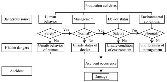
Figure 1.
Hidden danger induced accident mechanism in coal mines.
From the formation and development mechanism of hidden dangers, it can be known that, hidden dangers appear random, uncertain, and sudden, but they are by nature regular and predictable. Due to their uncertainty, this paper at first employs the gray system theory to probe into the time law of hidden danger quantity, and to predict their change trend. Subsequently, a gray prediction model for hidden danger quantity is established. Then, as to their randomness, the paper adopts the extreme learning machine to correct the residual error of the gray prediction model. The prediction principle is illustrated in Figure 2.
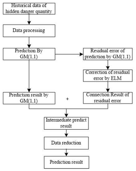
Figure 2.
Hidden danger quantity prediction principle. GM, gray model; ELM, extreme learning machine.
2.2. GM (1,1) Model Predicting Hidden Danger Quantity
2.2.1. Mean GM (1,1) Prediction Model
The gray system was proposed by a Chinese scholar named Deng Julong in 1982. It is a mathematical tool that explores uncertain problem of not having much data and information. The approach functions to extract valuable information from some known information, and realizes correct description and effective monitoring of system behaviors and evolution law [18]. By raw data processing and gray model establishment, gray prediction extracts, reveals, and knows the evolution law of the system, and makes quantitative prediction of the future status of the system. GM (1,1) model is the underlying model of gray prediction theory, and also the most popular gray prediction model. The model is further divided into GM (1,1) even gray model (EGM), GM (1,1) original differential gray model (ODGM), GM (1,1) even differential gray model (EDGM), and GM (1,1) discrete gray model (DGM). Relative to other three models, EGM is more suitable for an oscillating sequence [19,20,21]. Because there exists a lot of influential factors behind hidden dangers in each coal mine area, and are affected by technical and managerial aspects in the capability of identifying and screening them, the sequence formed by the quantity of loopholes identified in a coal mine every month is an oscillating sequence. Therefore, this paper chooses GM (1,1) EGM. Its underlying principle is [22,23,24,25]:
Suppose the original sequence is:
m is the size of samples.
For , for X, do first-order accumulation to get first-order accumulation to generate a sequence of sequences (1-AGO) and obtain , and
Figure out the nearest neighbor mean Z(1)(t) of , and
Then,
The whitening differential equation of the above equation is
The vector in the equation can be determined by least squares method, namely, , and
In the equation, a is known as development coefficient, which reflects the development status of a variable. b is known as gray actuating quantity.
Once each coefficient is figured out, gray GM (1,1) prediction model is determined
Then, inverse accumulation is made for the above equation, and the prediction value of any given input is worked out
2.2.2. Buffer Operator Improvement GM (1,1)
The hidden dangers in a coal mine are artificially identified and entered. The quantity of each month shows a significant volatility and randomness according to the feature analysis of the hidden dangers and the difference of individuals’ hidden dangers identification capability. Though the data are scattered, they always possess an overall function according to the characteristics of the hidden dangers in the system of each area. In order to weaken the randomness of the sequence, the sequence, formed by the mean of the hidden danger quantity of each N consecutive months, is considered as a new gray sequence according to the identification characteristics. That is to say, the initial hidden danger quantity sequence in Equation (1) is generated the operator D by using the mean, that is, through the operation of formula (10) and a new sequence is obtained.
And
Then use mean GM (1,1) model for prediction.
2.3. Residual Error Modified Model for Hidden Danger Prediction Based on PSO-RELM
2.3.1. ELM
Neural network has strong nonlinear fitting capability. It can better establish the quantitative relation of all factors in the system even if the qualitative relation of all the factors remains unknown [26,27,28,29]. Extreme learning machine in the neural network has been extensively used in the past years due to its simple structure, short training time, and high prediction precision. Hence, this paper adopts ELM to correct the residual error of gray GM (1,1) hidden danger quantity prediction.
Suppose there are N training samples , where Xi = [xi1, xi1, ⋯ xin]T ∈ Rn is the input value, and ti = [ti1, ti1, ⋯ tin]T ∈ Rn is the output value, then the regression model of the neuron function of which the hidden node number is L can be expressed as [30]:
where, f(x) is hidden activation function, is input weight, is output weight, and is the biased value of the ith hidden node.
The solving objective of the neural network is to obtain the least error output, namely, to make
That is, there exists , and , which make
Rewrite the above equation into a matrix form
Where, is the output of hidden node, and
is the weight of output layer, and
T is expected output vector, and
In order to give the minimal error between input value and target value, the equivalent minimal loss function is
Among ELM neural network algorithm, once input weight and hidden biased value are determined at random, the solution of the hidden output matrix is exclusively determined. Then the question is translated to solve . According to the mathematical theory, obtain
Where H+ is the generalized inverse of matrix , and
Moreover, we can prove that the norm of the solution obtained is minimal and exclusive. Hence, for given input value , its prediction value can be obtained
2.3.2. Regular Learning Machine RELM
Extreme learning machine (ELM) has the advantages of fast learning speed, etc. The solution obtained in Section 2.3.1 is the model established according to the least squares loss function, which only takes into account the least training error, namely, empirical risk. In statistics, the risk of the model consists of empirical risk and structural risk. Empirical risk reflects the training precision of the model, while structural risk reflects the generalization performance. The two combined determine the prediction precision of the model [31]. A sound model can not only obtain the training precision with better correctness, but satisfactory testing and prediction precision. That is to say, the model should avoid under-learning and over-learning. A study revealed that the smaller the weighted norm of feed forward neural network is, the more stable its network is, and the better its generalization performance is. As a result, the loss function of ELM neural network is translated into [32,33]. This method can overcome the above disadvantages, that is, the regular learning machine (RELM).
where, is empirical risk, is structural risk, and is weight coefficient. The above problem is transformed into resolving the extremum by Lagrange.
It is known that
Resolve
2.3.3. PSO-RELM
The initial weight and hidden deviation of the extreme learning machine are determined at random, so the resulting model is just the optimal prediction model at given initial weight and hidden deviation. Therefore, this paper adopts particle swarm optimization (PSO) to optimize the initial weight and hidden deviation.
PSO was first proposed by Eberhart and Kennedy in 1995, which was intended to study the foraging behavior of bird swarm. Namely, in a specific scenario, a bird swarm is searching for food at random, each of the birds can be considered as a particle, neither of the birds knows where the food is, but they know how far their location is to the food. Then, all the birds will search toward the bird currently nearest to the food and also toward their position historically nearest to the food [34].
In PSO, each particle is the feasible solution of the problem. Each particle owns an adaptive value determined by the target function and the velocity value determining the flight direction and distance of the particle [35,36]. In D-dimensional space, suppose the number of particles is M, and suppose the global optimal position at t is
Then, the historical optimal position of ith particle at t is
Then, the velocity of the ith particle at t+1 is
where, is inertial weight, are acceleration factor, normally 2, are random number between 0 and 1.
The position of the ith particle at t+1 is
This paper adopts PSO to optimize the initial weight and hidden deviation of ELM. The process is [37].
Step 1: A swarm is produced and maximal iterations are set. This paper sets the swarm at 20, and maximal iterations at 50. Each particle is composed of input weight and hidden deviation.
Step 2: For each individual particle, its output matrix is worked out by RELM algorithm. Then the root-mean-square error is obtained. The error is treated as fitness function. Each particle’s fitness value is computed. The individual and global optimal fitness particle’s parameter values are reserved.
Step 3: According to Equations (28) and (29), update the velocity and parameters of each particle.
Step 4: If maximal iterations are reached, computation ceases. The global optimal particle’s parameter values are considered as the parameters of the initial weight value and hidden deviation value of ELM. Otherwise, jump to Step 2.
3. Results and Analysis
This paper chooses the loophole quantity of a coal mine in seventeen consecutive months since January 2014 for the experiment. The original sequence is: X(0) =(777, 681, 715, 500, 762, 759, 627, 609, 392, 730, 690, 643, 550, 602, 604, 629, 611, 649, 493, 510, 466, 603, 581, 621). The first 22 numbers are training sample data, and the last 2 ones are testing sample data.
3.1. Predicting the Hidden Danger Quantity by GM (1,1) with Weakened Buffer Operator
According to artificial hidden danger identification characteristics and hidden danger development law, the mean of hidden danger quantity of every four months is treated as a new sequence value and a buffer operator sequence is generated according to Equation (10). The fitted values and errors of the original sequence and buffer operator sequence are listed in Table 1. The prediction values and errors of the original sequence and buffer operator sequence are listed in Table 2.

Table 1.
The GM (1,1) fitted value of original sequence and buffer operator sequence.
Table 2.
GM (1,1) prediction values of original sequence and buffer operator sequence.
The main parameters of GM (1,1) prediction model established by the original sequence are: development coefficient a = 0.011; gray actuation quantity b = 693.052; average relative error is 12.150%.
The main parameters of GM (1,1) prediction model established by the buffer operator sequence are: development coefficient a = 0.011; gray actuation quantity b = 684.769; average relative error is 3.749%.
The computation results show that, compared with the original sequence, the precision of the fitted values of the GM (1,1) prediction model established by the buffer operator sequence is obviously improved, and the oscillation is markedly weakened.
3.2. Modification of Residual Error Based on PSO-ELM
The experimental environment is Matlab2016b. Hidden set function is Sig. Regularization parameter uses 0.01. At first, we adopted RELM to optimize the hidden layer node. Then, we used RELM to optimize the initial swarm and maximal iterations of particle swarm algorithm. Finally, we employed PSO-RELM for experimental analysis.
(1) Determination of particle swarm parameters
The larger the number of swarms is, the more the iterations it takes, the smaller the resulting error is, the more complex the training devoted, and the longer the time it takes. A good model should be simple as far as possible while the precision is met. RELM is used to test the error of the model with different swarm numbers. The trained mean square error of the model is considered as an adaptive function. Table 3 and Figure 3 list the favorable errors and consumed time in case of different swarm numbers. (The errors are normalized errors.)
Table 3.
Time consumed and ultimate errors of the model with different swarm numbers.
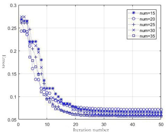
Figure 3.
Convergence graph of the errors of the model with different swarm numbers.
It is observed from Figure 3 and Table 3 that when the initial swarms are increased to a given number, the increased precision slows down, but the time consumed for the training of the model is largely linearly increased. Meanwhile, when the number of iterations reaches 20, the precision remains basically unchanged. Therefore, this paper chooses initial swarm number at 25, and maximal iteration number at 25.
(2) Optimization of hidden layer node parameters
Generally speaking, the more the hidden layer nodes, the more extract the fitted values, and the more complex the network. However, excessive hidden layer nodes may cause over-learning of the network, worsening its normalization capability. Table 4 separately tests the training error and consumed time of different hidden layer nodes.
Table 4.
Errors and consumed time of the model with different hidden layer nodes.
It is shown in Table 4 that with an increasing number of hidden layer nodes, the errors of the training generally becomes smaller and smaller, and time consumed longer and longer, suggesting that the more complex the network is, the longer the computation takes. However, the prediction precision does not improve continuously with the increasing of the number of hidden layer nodes. This indicates that more hidden layer nodes will not necessarily bring about improved precision of the model.
(3) Experiments
According to the analysis above, the number of initial swarms is set at 25, the number of maximal iterations is set at 25, and the data of the residual errors of every three months slide to generate the sample. The experimental environment is Matlab2016b. SIG is chosen as the hidden layer aggregation function. Normalization parameter is chosen as 0.01, and the number of hidden layer nodes is chosen as 7. After a lot of experiments, the mean of any ten prediction models is taken as the correction value of residual error. Table 5 lists the fitted values of the combination model. Table 6 lists the prediction values of the combination model. Table 7 lists the prediction values recovered as the hidden danger quantity of every month.
Table 5.
Fitted values of average hidden danger quantity of a coal mine.
Table 6.
Prediction value of average hidden danger quantity of a coal mine.
Table 7.
Prediction values of hidden danger quantity of a coal mine.
From Table 5, it can be known that GM (1,1) prediction model using buffer operator optimization largely fits the law of average hidden danger quantity of the mine for every four months. However, the stability of the hidden danger quantity is poor, and fitting precision is not sound, and some errors are even more than 7%. The precision is obviously improved after PSO-ELM model is used to correct the residual error. From Table 6 it is evident that the precision of the prediction values obtained by the model is high. As indicated in Table 7, when the mean of hidden danger quantity is translated to the hidden danger quantity of every month, the prediction precision somewhat decreases, but the error is still below 5%. Hence, using gray neural network to optimize the combination model is more suitable for the hidden danger quantity of a coal mine.
4. Discussion
On the one hand, the accurate prediction of the number of hidden dangers can reveal the overall safety status of the mine, on the other hand, it can guide the formulation and implementation of the hidden trouble detection plan, which is of great significance to the coal mine safety production control. For the forecast model and its prediction results in this article, we will discuss from the following aspects:
First of all, from the above experimental results, we can see that the relative error of the prediction results is 12.5% when mean GM (1,1) prediction model is adopted, the relative error of the prediction results is 3.749% when buffer operator improvement GM (1,1) is adopted, and the relative error of the prediction results is 3.24% when the buffer operator improvement GM (1,1)+PSO-RELM model is used. The relative error of the last two prediction models is less than 5%, which shows that the two models can better predict the number of coal mine hazards.
Secondly, hidden danger is the unsafe state of human, material, environment, and management, which exists objectively, but it is found out manually. Therefore, the number of hidden dangers found out every month in the coal mine is limited by management level and other factors, and there is a certain subjectivity, which brings great difficulties to the prediction. As shown in Table 7, taking the average number of hidden dangers for three consecutive months as the prediction quantity, the relative error of the prediction result is reduced to 0.875%, which shows that it can weaken the random influence of the number of hidden dangers caused by human factors to a certain extent.
Finally, the number of hidden dangers on the one hand is affected by the development law of the hidden danger itself, on the other hand, it is also affected by other external factors, such as the change of geological conditions, the transformation of coal mining technology [38,39,40], etc. The model adopted in this paper belongs to the scope of the time series prediction model. The time series prediction model only shows good results in the simulation of the sequence itself. In other words, the prediction model used in this study cannot reflect the impact of other factors on the system in time. Ignoring the changes of internal factors may lead to inaccurate prediction. For example, when the mine is shut down for rectification, the number of hidden dangers will sharply reduce and when an accident occurs in a coal mine, the number of hidden dangers will increase significantly, which needs to be overcome in the future research.
5. Conclusions
(1) Prediction of the number of hidden dangers in coal mines plays an important role in the management of coal mine enterprises to better understand the situation of production safety in each area of the coal mine. It can judge the authenticity of the number of hidden dangers and reduce the number of hidden dangers. According to the mechanism analysis of the formation and development of hidden dangers, this paper knows that its essence is regular and predictable.
(2) The combination model of gray system theory and artificial neural network was used to predict the number of hidden dangers in coal mines. The model is based on the mean GM (1,1) model, which requires fewer samples, and is simple to calculate. The number of hidden dangers of average consecutive months is used as a buffer operator to weaken the oscillation of the original sequence, which improves the accuracy of model prediction.
(3) The regularization parameter term is used to optimize the ELM to improve the generalization ability of the model. Besides, the PSO is used to optimize the initial weight and hidden layer deviation of the ELM, so as to obtain a better training model, make the model more stable, and have higher prediction accuracy.
(4) The gray neural network prediction model is adopted, which has low requirements for data samples. It combines the advantages of two prediction methods, that is, it reflects the complex gray system behavior of hidden dangers in coal mines, and can dynamically predict.
Author Contributions
Conceptualization, H.Z. and Q.H.; methodology, H.Z.; software, Q.H.; validation, H.Z., Q.H. and Z.W.; formal analysis, Q.H.; investigation, Z.W.; resources, L.Z.; data curation, L.Z.; writing—original draft preparation, Q.H.; writing—review and editing, H.Z.; visualization, Z.W.; supervision, H.Z.; project administration, H.Z.; funding acquisition, H.Z. All authors have read and agreed to the published version of the manuscript.
Funding
This research was funded by [National Key Research and Development Program of China] grant number [2018YFC0808301]. And the APC was funded by [National Key Research and Development Program of China].
Conflicts of Interest
The authors declare no conflict of interest.
References
- Li, T. Study On investigation and management system for safety hidden dangers and internal control processes in coal mines. China Coal 2012, 2, 26–29. [Google Scholar]
- Liang, Z.; Xin, G.; Guanglong, L.; Jian, J. Discussion on three works relationships of hidden trouble investigation and control and safety quality standardization and safety risk prevention and control management system. China Coal 2015, 7, 116–119. [Google Scholar]
- Zhang, D.W. Analysis of Coal Mine Safety Hidden Danger Trends Based on OLAM. Coal Eng. 2015, 5, 139–142. [Google Scholar]
- Zhang, S.Y. Research and Practice of Coal Mine Safety Hidden Trouble Investigation and Control. Zhongzhou Coal 2010, 11, 113–114. [Google Scholar]
- General Office of State Security supervision. Circular of the General Office of the State Administration of Work Safety on Further Doing Hidden Danger Elimination and Control Normalization Mechanism Construction Pilot Work. For. Labor Saf. 2013, 26, 26–27. [Google Scholar]
- Chen, Y.Q. Application of data mining technology in coal mine hidden hazard management. Ind. Mine Autom. 2016, 42, 27–30. [Google Scholar]
- Zhang, C.L. Study On big data processing and knowledge discovery analysis method for safety hazard in coal mine. J. Saf. Sci. Technol. 2016, 09, 176–181. [Google Scholar]
- Wang, X.Y. The Study of Evaluation and Prediction on the Governance Capability for Safety Hidden Danger of Coal Mine. Ph.D. Thesis, China University of Mining and Technology (Beijing), Beijing, China, 2013. [Google Scholar]
- Chen, Q. Analysis on Accident Causation Factors and Hazard Theory. China Saf. Sci. J. 2009, 19, 67–71. [Google Scholar]
- Wang, L.K. The Hierarchy Analysis for Hidden Danger and Research on Early Warning Method in Coal Mine. Ph.D. Thesis, China University of Mining and Technology (Beijing), Beijing, China, 2015. [Google Scholar]
- Zhang, D. Studies on the Identification of Mine Safety Hidden Danger and The Closed-Loop Management Model. Ph.D. Thesis, China University of Mining and Technology (Beijing), Beijing, China, 2009. [Google Scholar]
- Fan, Y. Research on Neural Network Prediction. Master’s Thesis, Southwest Jiao Tong University, Chengdu, China, 2005. [Google Scholar]
- Gao, W.; Farahani, M.R.; Aslam, A.; Hosamani, S. Distance learning techniques for ontology similarity measuring and ontology mapping. Clust. Comput. J. Netw. Softw. Tools Appl. 2017, 20, 959–968. [Google Scholar] [CrossRef]
- Xiong, Z.G.; Wu, Y.; Ye, C.H.; Zhang, X.M.; Xu, F. Color image chaos encryption algorithm combining CRC and nine palace map. Multimed. Tools Appl. 2019, 78, 31035–31055. [Google Scholar] [CrossRef]
- Zhao, N.; Xia, M.J.; Mi, W.J. Modeling and solution for inbound container storage assignment problem in dual cycling mode. Discret. Contin. Dyn. Syst. S 2020. [Google Scholar] [CrossRef]
- Yu, K.; Zhou, L.; Cao, Q.; Li, Z. Evolutionary Game Research on Symmetry of Workers’ Behavior in Coal Mine Enterprises. Symmetry 2019, 11, 156. [Google Scholar] [CrossRef]
- Chen, B.Z.; Wu, M. Etiologies of accident and Safety concepts. J. Saf. Sci. Technol. 2008, 4, 42–46. [Google Scholar]
- Tian, S.C.; Li, H.X.; Wang, L.; Chen, T. Probe into the Frequency of Coal Mine Accidents Based on the Theory of Three Types of Hazards. China Saf. Sci. J. 2007, 17, 177–179. [Google Scholar]
- Den, J.L. Brief Introduction of Grey System Theory. Inn. Mong. Electr. Power 1993, 3, 51–52. [Google Scholar]
- Liu, S.F.; Zeng, B.; Liu, J.F.; Xie, N.M. Several Basic Models of GM (1,1) and Their Applicable Bound. J. Syst. Eng. Electron. 2014, 3, 501–508. [Google Scholar]
- Liu, S.F.; Yang, Y.J.; Wu, L.F. Grey System Theory and Its Application; Science Press: Beijing, China, 2014. [Google Scholar]
- Chen, L.; Lin, W.; Li, J.; Tian, B.; Pan, H. Prediction of lithium-ion battery capacity with metabolic grey model. Energy 2016, 106, 662–672. [Google Scholar] [CrossRef]
- Kumar, U.; Jain, V.K. Time Series Models (Grey-Markov, Grey Model with Rolling Mechanism and Singular Spectrum Analysis) to Forecast Energy Consumption in India. Energy 2010, 35, 1709–1716. [Google Scholar] [CrossRef]
- Shaikh, F.; Ji, Q.; Shaikh, P.H.; Mirjat, N.H.; Uqaili, M.A. Forecasting China’s Natural Gas Demand Based on Optimised Nonlinear Grey Models. Energy 2017, 140, 941–951. [Google Scholar] [CrossRef]
- Zhou, H.P. The Research and Application of Death Rate Per Million-Ton Coal Prediction Method. Ph.D. Thesis, China University of Mining and Technology (Beijing), Beijing, China, 2012. [Google Scholar]
- Jiao, L.C.; Yang, S.Y.; Liu, F.; Wang, S.G.; Feng, Z.X. Seventy Years Beyond Neural Networks: Retrospect and Prospect. Chin. J. Comput. 2016, 8, 1697–1716. [Google Scholar]
- Chen, J.H.; Liu, L.; Zhou, Z.Y.; Yong, X.Y. Optimization of mining methods based on combination of principal component analysis and neural networks. J. Cent. South Univ. 2010, 41, 1967–1972. [Google Scholar]
- Wu, A.X.; Guo, L.; Yu, J.; Yang, Y.P.; Xiao, X. Neural network model construction and its application in fuzzily optimization of mining method. Min. Met. Eng. 2003, 23, 6–11. [Google Scholar]
- Kennedy, J. Particle Swarm Optimization. In Encyclopedia of Machine Learning; Sammut, C., Webb, G.I., Eds.; Springer: Boston, MA, USA, 2011. [Google Scholar]
- Huang, G.B.; Zhu, Q.Y.; Siew, C.K. Extreme Learning Machine: Theory and Applications. Neurocomputing 2006, 70, 489–501. [Google Scholar] [CrossRef]
- Lan, Y.; Yeng, C.S.; Huang, G.B. Ensemble of Online Sequential Extreme Learning Machine. Neurocomputing 2009, 72, 3391–3395. [Google Scholar] [CrossRef]
- Bartlett, P.L. The Sample Complexity of Pattern Classification with Neural Networks: The Size of the Weights Is More Important Than the Size of the Network. Ieee Trans. Inf. Theory 1998, 44, 525–536. [Google Scholar] [CrossRef]
- Deng, W.Y.; Zheng, Q.H.; Lin, C. Regularized Extreme Learning Machine. In Proceedings of the 2009 IEEE Symposium on Computational Intelligence and Data Mining, Nashville, TN, USA, 30 March–2 April 2009; pp. 389–395. [Google Scholar]
- Xue, H.B.; Lun, S.X. A Review on Application of PSO in Multi Objective Optimization. J. Bohai Univ. (Nat. Sci. Ed.) 2009, 3, 265–269. [Google Scholar]
- Zhang, Y.; Le, J.; Liao, X.; Zheng, F.; Liu, K.; An, X. Multi-objective hydro-thermal-wind coordination scheduling integrated with large-scale electric vehicles using IMOPSO. Renew. Energy 2018, 128, 91–107. [Google Scholar]
- Yang, X.Y.; Guan, W.Y.; Liu, Y.Q.; Xiao, Y.Q. Prediction Intervals Forecasts of Wind Power Based on PSO-KELM. Proc. Chin. Soc. Electr. Eng. 2015, S1, 146–153. [Google Scholar]
- Wang, J.; Bi, H.Y. A New Extreme Learning Machine Optimized by PSO. J. Zhengzhou Univ. (Nat. Sci. Ed.) 2013, 1, 100–104. [Google Scholar]
- Box, G.E.P.; Jenkins, G. Time Series Analysis, Forecasting and Control; Holden-Day, Incorporated: San Francisco, CA, USA, 1990; pp. 238–242. [Google Scholar]
- Bajić, S.; Bajić, D.; Gluščević, B.; Ristić Vakanjac, V. Application of Fuzzy Analytic Hierarchy Process to Underground Mining Method Selection. Symmetry 2020, 12, 192. [Google Scholar] [CrossRef]
- Tsolaki-Fiaka, S.; Bathrellos, G.D.; Skilodimou, H.D. Multi-Criteria Decision Analysis for an Abandoned Quarry in the Evros Region (NE Greece). Land 2018, 7, 43. [Google Scholar] [CrossRef]
© 2020 by the authors. Licensee MDPI, Basel, Switzerland. This article is an open access article distributed under the terms and conditions of the Creative Commons Attribution (CC BY) license (http://creativecommons.org/licenses/by/4.0/).