Abstract
This paper analyzes the operation principle and predicted value of the recurrent-neural-network (RNN) structure, which is the most basic and suitable for the change of time in the structure of a neural network for various types of artificial intelligence (AI). In particular, an RNN in which all connections are symmetric guarantees that it will converge. The operating principle of a RNN is based on linear data combinations and is composed through the synthesis of nonlinear activation functions. Linear combined data are similar to the autoregressive-moving average (ARMA) method of statistical processing. However, distortion due to the nonlinear activation function in RNNs causes the predicted value to be different from the predicted ARMA value. Through this, we know the limit of the predicted value of an RNN and the range of prediction that changes according to the learning data. In addition to mathematical proofs, numerical experiments confirmed our claims.
1. Introduction
Artificial intelligence (AI) with machines are coming into our daily lives. In the near future, there will be no careers in a variety of fields, from driverless cars becoming commonplace, to personal-routine assistants, automatic response system (ARS) counsellors, and bank clerks. In the age of machines, it is only natural to let machines do the work [1,2,3,4,5], aiming for the operation principle of the machine and the direction of a machine’s prediction. In this paper, we analyzed the principles of operation and prediction through a recurrent neural network (RNN) [6,7,8].
The RNN is an AI methodology that handles incoming data in a time order. This methodology learns about time changes and predicts them. This predictability is possible because of the recurrent structure, and it produces similar results as the time series of general statistical processing [9,10,11,12]. We calculate the predicted value of a time series by calculating the general term of the recurrence relation. Unfortunately, the RNN calculation method is very similar to that of the time series, but the activation function in a neural-network (NN) structure is a nonlinear function, so nonlinear effects appear in the prediction part. For this reason, it is very difficult to find the predicted value of a RNN. However, due to the advantages of the recurrent structure and the development of artificial-neural-network (ANN) calculation methods, the accuracy of predicted values is improving. This led to better development and greater demand for artificial neural networks (ANNs) based on RNNs. For example, long short-term memory (LSTM), gated recurrent units (GRU), and R-RNNs [13,14,15,16] start from a RNN and are used in various fields. In other words, RNN-based artificial neural networks are used in learning about time changes and the predictions corresponding to them.
There are not many papers attempting to interpret the structure of recurrent structures, and results are also lacking. First, the recurrent structure is used to find the expected value by using it iteratively according to the order of data input over time. This is to predict future values from past data. In a situation where you do not know a future value, it is natural to use the information you know to predict the future. These logical methods include the time-series method in statistical processing, which is a numerical method. The RNN structure is very similar to the combination of these two methods. Autoregressive moving average (ARMA) in time series is a method of predicting future values by creating a recurrence relation by the linear combination of historical data. More details can be found in [17,18]. Taylor’s expanding RNN under certain constraints results in linear defects of historical data, such as the time series. More details are given in the text. From these results, this paper describes the range of the predicted value of a RNN.
2. RNN and ARMA Relationship
In this section, we explain how a RNN works by interpreting it. In particular, the RNN is based on the ARMA format in statistical processing. More details can be found in [19,20,21]. This is explained through the following process.
2.1. RNN
In this section, we explain RNN among various modified RNNs. For convenience, RNN refers to the basic RNN. The RNN that we deal with is
where t represents time, is a predicted value, is a real value, and is a hidden layer. The hidden layer is computed by
where is input data, and are real values, and is the previous hidden layer. For machine learning, let be the set of learning data, and let be the number of the size of . In other words, when the first departure time of learning data is 1, we can say that . Assuming that the initial condition of the hidden layer is 0 , we can compute for each time t. is data on time and is a predicted value, so we want to satisfy . Because unhappiness does not establish the equation, an error occurs between and . So, let and . Therefore, machine learning based on RNN is the process of finding , , and that can minimize error value E. We used , ,..., in learning data to find , , and that minimize error E, and used them to predict the values (, ,...) after time . More details can be found in [22,23,24,25].
2.2. ARMA in Time Series
People have long wanted to predict stocks. This required predictions from historical data on stocks, and various methods have been studied and utilized. In particular, the most widely and commonly used is the ARMA method, which was developed on the basis of statistics. This method simply creates a linear combination of historical data for the value to be predicted and calculates it on this basis.
where ,⋯, are given data, and we can calculate predicted value by calculating the values of , ⋯, , and . In order to obtain the values of , ⋯, , and , there are various methods, such as optimization by numerical data values, Yule–Walker estimation, and corelation calculation. This equation is used to predict future values through the calculation of general terms of the recurrence relation. More details can be found in [17].
2.3. RNN and ARMA
In RNN, the hidden layer is constructed by the hyperbolic tangent function that is
Function tanh is expanded:
where x is in . Using this fact and expanding ,
where is an error. Therefore,
Since the same process is repeated for ,
Repeatedly,
Therefore,
If is less than 0.1, the terms after the fourth order () are too small to affect the value to be predicted. Conversely, if is greater than 1, the value to be predicted increases exponentially. Under the assumption that we can expand hyperbolic tangent function (tanh), condition must be less than 1. Since we can change only , , and , the RNN can be written as
This equation is an ARMA of order 5. More details can be found in [18]. This development method was developed on the premise that the variable part of the tanh function is smaller than a specific value ( and ), and is limited in terms of utilization.
3. Analysis of Predicted Values
From the above section, , , , , and are fixed. Then, we obtained sequence by the following equality:
where and .
Theorem 1.
Sequence is bounded and has a converging subsequence.
Proof.
Since , for all l. Using the Arzela–Ascoli theorem, there exists a converging subsequence. More details can be found in [26]. □
In order to see the change in the value of , if the limit of is h, Equation (14) is written as . Therefore, as the values of and b, the value of h that satisfies this equation changes.
3.1. Limit Points of Prediction Values
We now analyze the convergence value of the sequence. In order to see the convergence of the sequence, we introduced the following functions:
For calculation convenience, this equation changes as follows.
where is an initial condition, the convergence of is , and satisfies Equation (17) (). Therefore, we have to look at the roots that satisfy the expression in Equation (17).
Theorem 2.
There should be at least one solution to Equation (17)
Proof.
Let . Function g is continuous and differentiable. If , then ; If , then . Therefore, there exists at least one solution. □
Theorem 3.
If , then the equation has just one solution.
Proof.
If , then . Therefore, g is a monotonically decreasing function. As a result of this, there exists only one solution satisfying . □
Under the assumption that the value of , two values satisfying necessarily exist. Therefore, assuming , we find and satisfying , and have assuming . Therefore, on , on , and on from computing g. Assuming and , we have and , respectively. From computing , is obtained.
Theorem 4.
Assuming , If or then, g has two solutions. If , then g has three solutions. If or , then g has one solution.
Proof.
This proof assumes that . If , then we know . Therefore, we have . Since is a monotonically decreasing function on , there exists a unique solution, such that . If , then we know . Therefore, we know , and there exists a unique solution, such that on for the same reason. So, if , we have two solutions. One is on and the other is . If , we have and . There are three solutions, such that on , on , and on . If , we know that . Therefore, since , and g is a monotonically decreasing function on , there is a solution satisfying . So, if , we have two solutions, such that and on . If , then . Since and g is a decrease function, there is a solution, such that on . □
In this section, we see the change in the number of solutions that satisfy Equation (17) as the values of and b change. The change of the sequence according to the initial condition of the sequence and according to the number of each solution of Equation (17) is explained.
Figure 1 shows the graph of and . If point (, b) is contained in the white region, there is one solution. If point (, b) lies in the red curve, there are two solutions. If point (, b) is contained in the blue region, there are three solutions. In Section 4, we plot point (a, b) in the solution number region to check for the number of solutions of each case.
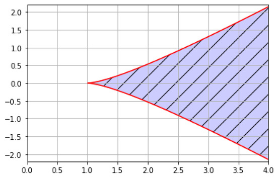
Figure 1.
Solution number region.
3.2. Change of Prediction Values (Sequence)
We examined the number of the solutions of g depending on the values of and b. In order to see the change of the predicted value according to the change of and b, Equation (14) was changed to , and sequence was obtained. Sequences , g, and have the following relationship: and . Therefore, the predicted value was obtained by and . The solutions of g are the limit points of sequence by using . One of the reasons we interpreted the predictions was to identify the movement condensation (the changing value) of the predictions. We saw various cases that made function g zero from the previous theorem. The change of the sequence according to initial condition in each case is explained.
Theorem 5.
Assuming and , sequence converged to , where satisfies .
Proof.
Under condition and , on and on . If then . From computing, is a monotonically increasing sequence. So, sequence converges to . If then . From computing, is a monotonically decreasing sequence. Therefore, sequence converged to . □
Theorem 6.
Assuming and , there exist two solutions and that satisfy . If , sequence converges to . If , sequence converges to ,
Proof.
on . So is a monotonically increasing sequence from computing. If , converges to ; if , converges to . On z □
Theorem 7.
Assuming and , if , converges to ; if , converges to , where is an initial condition.
Proof.
From computing , we have on , and on . Therefore sequence is a monotonically increasing sequence, and converges to . From , g is convex, and on , we have on . On we have and . Sequence is a monotonically decreasing sequence, and the convergence value is . With the same calculation, g is concave, and . Therefore, on and on . Sequence is a monotonically increasing sequence, and the convergence value is . If , . Therefore, on . Sequence is a monotonically decreasing sequence, and the convergence value is . □
Theorem 8.
Assuming and , there exist two solutions and that satisfy . If , sequence converges to . If , sequence converges to . If , sequence converges to ,
Proof.
If , . Therefore, sequence is a monotonically decreasing sequence. So, sequence converges to . If , . Therefore, sequence is a monotonically decreasing sequence. So, sequence converges to . If , . Therefore, sequence is a monotonically increasing sequence. So, sequence converges to . □
Theorem 9.
Assuming and , sequence converges to , where satisfies .
Proof.
Under conditions ( and ), . Therefore if then . Therefore, sequence is a monotonically decreasing sequence. So, sequence converges to . If , . Therefore, sequence is a monotonically increasing sequence. So, sequence converges to . □
Theorem 10.
Assuming , sequence converges to , where satisfies .
Proof.
Under condition (), has a unique solution satisfying . If , . Therefore, sequence is a monotonically increasing sequence. So, sequence converges to . If , . Therefore, sequence is a monotonically decreasing sequence. So, sequence converges to . □
In condition , function is an increasing function, and there is no change of the sign of . However, in condition , function is a decreasing function, and there is change of the sign of .
Theorem 11.
Assuming , sequence converges to , where satisfies .
Proof.
where is between and . Therefore,
Sequence is a that converges to □
Theorem 12.
Assuming , sequence converges to , where satisfies , or sequence vibrates.
Proof.
where is between and . Therefore,
If , sequence is a that converges to . If , sequence vibrates. □
4. Numerical Experiments
In this section, we confirmed the numerical results to identify RNN analysis interpreted in the previous section. As we saw in the previous section, RNN predictions appeared in three cases. Case 1 is Equation (17) that has one solution, Case 2 is Equation (17) that has two solutions, and Case 3 is Equation (17) that has three solutions. In Cases 1 to 3, we checked the number of solutions in Equation (17), and predicted the values according to the initial conditions. In Cases 4 through 7, experiments were conducted on the situation where learning data increase, learning data increase and decrease, learning data decrease and increase, and learning data vibrate. We obtained a picture from each numerical experiment. In each figure, (a) plots the RNN predictions and the learning data, the red curve is , (b) denotes and b in the area of existence of the solution, and (c) is a picture of z about Equation (17).
4.1. Case 1: One-Solution Case of Equation (17)
The situation with one solution was divided into the case where is less than 1 and is greater than 1.
4.1.1. Theta < 1
Let , , , , and . ∼ are learning data. In this case, we obtained , , , and . Therefore, and . The limit of the is (0.65).
In Figure 2a, are the black stars and are the prediction values (blue line). Figure 2b shows and . Figure 2c shows the result of Equation (17). In Figure 2c, * is . From Figure 2, we see that from the learning data, the solution of Equation (17) is one, initial value is 0.6, and is 0.5.
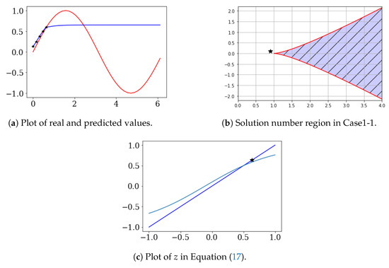
Figure 2.
One-solution case of Equation (17) (θ < 1).
4.1.2. Theta > 1
Let , , , , and . ∼ are learning data. In this case, we obtained , , , and . Therefore, and . The limit of is (0.64).
Figure 3 also shows results similar to those in Figure 2. Figure 3a shows and ( are the prediction values). Figure 3b shows and b. Figure 3c shows the result of Equation (17).
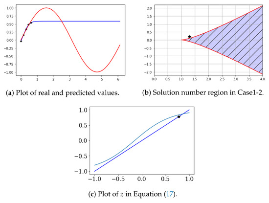
Figure 3.
One-solution case of Equation (17) (θ > 1).
4.2. Case 2: Two-Solution Case of Equation (17)
This situation is two solutions of Equation (17) by = (1.3, 0.101). Let , , , , and . ∼ are learning data. Figure 4 shows the solution number region and (black star). As shown in Figure 4, there are two solutions to Equation (17) from the learning data. In this situation, we conducted two experiments. The first case was initial condition existing between and . The second case was initial condition being less than . In the first case, the limited value of from the proof had to go to , and in the second case, the limited value of from the proof had to go to . This result was verified from the numerical experiments. The theory of the previous section was exempted through this numerical experiment.
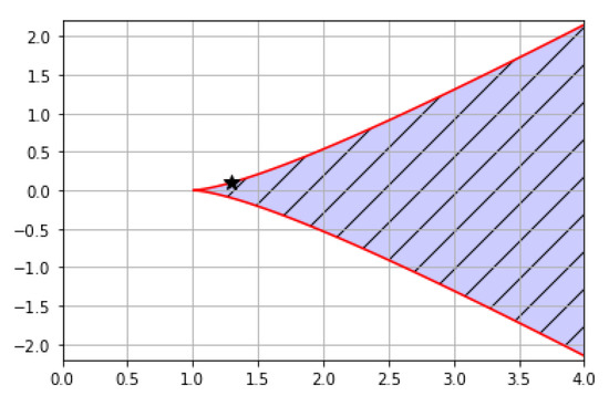
Figure 4.
Solution number region in Case 2.
4.2.1. First Case
In this case, we obtained , , , and . Therefore, and . The limit of is (0.47).
Figure 5a shows that are the black stars and are the prediction values (blue line). Figure 5b shows the result of Equation (17). In Figure 5b, * is , and is 0.71.
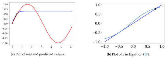
Figure 5.
Two-solution case of Equation (17).
4.2.2. Second Case
In this case, we obtained , , , and . Therefore, and . The limit of is (0.2).
Figure 6a shows that are the black stars and are the prediction values (blue line). Figure 6b shows the result of Equation (17). In Figure 6b, * is , and is −0.34.
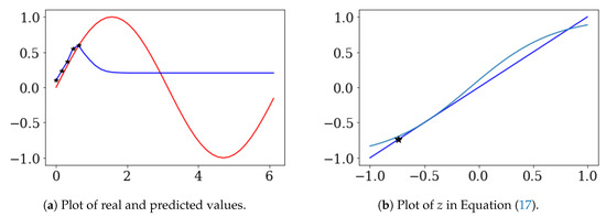
Figure 6.
Two-solution case of Equation (17).
4.3. Case 3: Three-Solution case of Equation (17)
This situation is three solutions of Equation (17) by = (2, 0.1). Let , , , , and . ∼ are learning data. Figure 7 shows the solution number region and (black star). As shown in Figure 7, there are three solutions from the learning data. In this situation, we conducted two experiments. For convenience, the three roots are indicated by , , and , respectively, as in the notation above. The first case was initial condition existing between and . The second case is initial condition existing between and . In the first case, the limited value of from the proof had to go to , and in the second case, the limited value of from the proof had to go to . This result was verified from the numerical experiments. The theory of the previous section was exempted through numerical experiments.
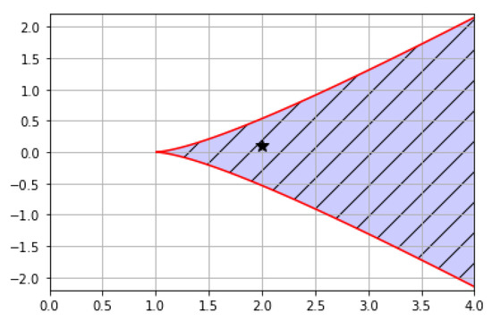
Figure 7.
Solution number region in Case 3.
4.3.1. First Case
In this case, we obtained , , , and . Therefore, and . The limit of the is (0.58).
In Figure 8a, are the black stars and are the prediction values (blue line). Figure 8b shows the result of Equation (17). In Figure 8b, * is , and is 0.79.
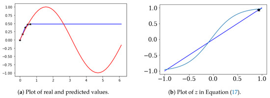
Figure 8.
Three-solution case of Equation (17).
4.3.2. Second Case
In this case, we obtained , , , , and . Therefore, and . The limit of is (1.03).
In Figure 9a, are the black stars and are the prediction values (blue line). Figure 9b shows the result of Equation (17). In Figure 5b, * is , and is −0.86.
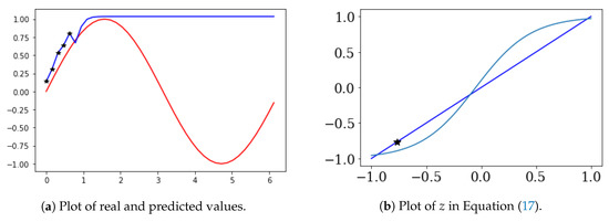
Figure 9.
Three-solution case of Equation (17).
4.4. Case 4: Learning Data Increase
Let , , , , and . ∼ are learning data. In this case, we obtained , , , , and . Therefore, and . The limit of is (0.93).
In Figure 10a, are the black stars and are the prediction values (blue line). Figure 10b shows and b. Figure 10c shows the result of Equation (17). In this case, . From and b, Equation (17) has one solution. As can be seen in Figure 10, learning data increased and converged to a specific value.
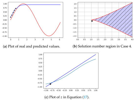
Figure 10.
Learning data increase.
4.5. Case 5: Learning Data Increase and Decrease
Let , , , , and . ∼ are learning data. In this case, we obtained , , , , and . Therefore, and . The limit of is (0.97).
In Figure 11a, are the black stars and are the prediction values (blue line). Figure 11b shows and b. Figure 11c shows the result of Equation (17). In this case, . From and b, Equation (17) has one solution. As can be seen in Figure 11, the training data converged to a specific value after increasing and decreasing. From and b, Equation (17) has one solution. As can be seen in Figure 11, the average value of the learning data gave the predicted value.
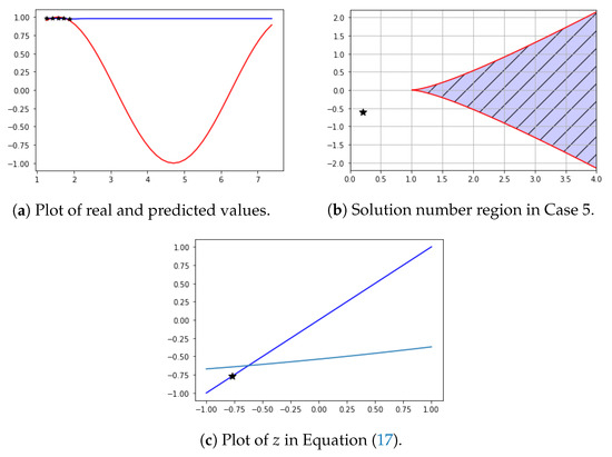
Figure 11.
Learning data increase and decrease.
4.6. Case 6: Learning Data Decrease and Increase
Let , , , , and . ∼ are learning data. In this case, we obtained , , , , and . Therefore, and . The limit of is (-0.97).
In Figure 12a, are the black stars and are the prediction values (blue line). Figure 12b shows and b. Figure 12c shows the result of Equation (17). In this case, . From and b, Equation (17) has one solution. As can be seen in the Figure 12, data increased and converged to a specific value. From and b, Equation (17) has one solution. As can be seen in Figure 12, the average value of the learning data gave the predicted value.
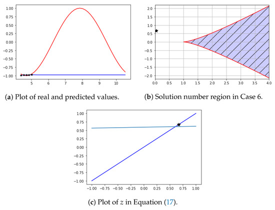
Figure 12.
Learning data decrease and increase.
4.7. Case 7: Learning Data Vibrate
Let , , , , and . ∼ are learning data. In this case, we obtained , , , , and . Therefore, and The limit of is (0.5).
In Figure 13a, are the green circles, are the black stars, and are the prediction values (blue line). In Figure 13a, the reason that the value of learning data () and the values of the learning result () are different is that the RNN structure was simple, and sufficient learning was not achieved. In future work, we aim to study the RNN structure to learn these complex learning data well. Figure 13b shows and b. Figure 13c shows the result of Equation (17). In this case, . From and b, Equation (17) has one solution. As can be seen in Figure 13, data increased and converged to a specific value. In this case of and b, the solution of Equation (17) should be one. However, two contents are contradictory because learning data should be presented in two cases, 1 and −1. As a result, the cost function only increased.
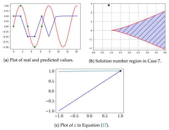
Figure 13.
Learning data vibrate.
5. Conclusions
In this paper, we interpreted the structure of the underlying the RNN and, on this basis, we found the principles that the RNN could predict. A basic RNN works like a time series in a very narrow range of variables. In a general range, a nonlinear function of which the maximum and minimum are specified causes the value of a function to fall within an iterative range. Because the function value is repeated within a certain range, the predicted value behaves like fixed-point iteration. In other words, we used the tanh (activation) function, so that the value was in the range of −1 to 1, and the absolute value of the predicted value in this range was less than 1. As a result, as the prediction value was repeated, the prediction value converged to a specific value. Through this paper, we found that the basic operating principle of a RNN is the operation principle of the time series, which we know as linear analysis and fixed-point iteration, which is nonlinear. In general, the solution of Equation (17) was one of the numerical calculations. Therefore, the present structure could not be solved in the case of numerical experiment Case 7 (learning data vibration). To solve this problem, it is necessary to diversify the structure, increase the number of layers, and switch to a vector structure. Next, we aim to further study RNNs in vector structures.
Author Contributions
Conceptualization, J.P. and D.Y.; Data curation, J.P.; Formal analysis, D.Y.; Funding acquisition, D.Y.; Investigation, J.P.; Methodology, D.Y. and S.J.; Project administration, J.P. and D.Y.; Resources, J.P.; Software, S.J.; Supervision, S.J.; Validation, S.J.; Visualization, S.J.; Writing—original draft, D.Y.; Writing—review & editing, J.P. and S.J. All authors have read and agreed to the published version of the manuscript.
Funding
This work was supported by the Basic Science Research Program through the National Research Foundation of Korea (NRF), funded by the Ministry of Education, Science, and Technology (grant number NRF-2017R1E1A1A03070311).
Acknowledgments
We sincerely thank the anonymous reviewers whose suggestions helped to greatly improve and clarify this manuscript.
Conflicts of Interest
The authors declare no conflict of interest.
References
- Rumelhart, D.E.; Hinton, G.E.; Williams, R.J. Learning representations by back-propagating errors. Nature 1986, 323, 533–536. [Google Scholar] [CrossRef]
- Werbos, P.J. Generalization of backpropagation with application to a recurrent gas market model. Neural Netw. 1988, 1, 339–356. [Google Scholar] [CrossRef]
- Schmidhuber, J. A Local Learning Algorithm for Dynamic Feedforward and Recurrent Networks. Connect. Sci. 1989, 1, 403–412. [Google Scholar] [CrossRef]
- Cho, K.; Merrienboer, B.V.; Bahdanau, D.; Bengio, Y. On the Properties of Neural Machine Translation: Encoder-Decoder Approaches. arXiv 2014, arXiv:1409.1259. [Google Scholar]
- Jin, Z.; Zhou, G.; Gao, D.; Zhang, Y. EEG classification using sparse Bayesian extreme learning machine for brain—Computer interface. Neural Comput. Appl. 2018, 1–9. [Google Scholar] [CrossRef]
- Schmidhuber, J. A Fixed Size Storage O(n3) Time Complexity Learning Algorithm for Fully Recurrent Continually Running Networks. Neural Comput. 1992, 4, 243–248. [Google Scholar] [CrossRef]
- Pascanu, R.; Mikolov, T.; Bengio, Y. On the difficulty of training recurrent neural networks. In Proceedings of the 30th International Conference on Machine Learning (ICML 2013), Atlanta, GA, USA, 16–21 June 2013; pp. 1310–1318. [Google Scholar]
- Cho, K.; Merrienboer, B.V.; Gulcehre, C.; Bahdanau, D.; Bougares, F.; Schwenk, H.; Bengio, Y. Learning Phrase Representations using RNN Encoder-Decoder for Statistical Machine Translation. arXiv 2014, arXiv:1406.1078. [Google Scholar]
- Dangelmayr, G.; Gadaleta, S.; Hundley, D.; Kirby, M. Time series prediction by estimating markov probabilities through topology preserving maps. In Applications and Science of Neural Networks, Fuzzy Systems, and Evolutionary Computation II; International Society for Optics and Photonics: Bellingham, WA, USA, 1999; Volume 3812, pp. 86–93. [Google Scholar]
- Wang, P.; Wang, H.; Wang, W. Finding semantics in time series. In Proceedings of the 2011 ACM SIGMOD International Conference on Management of Data, Athens, Greece, 12–16 June 2011; pp. 385–396. [Google Scholar]
- Afolabi, D.; Guan, S.; Man, K.L.; Wong, P.W.H.; Zhao, X. Hierarchical Meta-Learning in Time Series Forecasting for Improved Inference-Less Machine Learning. Symmetry 2017, 9, 283. [Google Scholar] [CrossRef]
- Xu, X.; Ren, W. A Hybrid Model Based on a Two-Layer Decomposition Approach and an Optimized Neural Network for Chaotic Time Series Prediction. Symmetry 2019, 11, 610. [Google Scholar] [CrossRef]
- Bengio, Y.; Simard, P.; Frasconi, P. Learning long-term dependencies with gradient descent is difficult. IEEE Trans. Neural Netw. 1994, 5, 157–166. [Google Scholar] [CrossRef]
- Hochreiter, S.; Schmidhuber, J. Long Short-Term Memory. Neural Comput. 1997, 9, 1735–1780. [Google Scholar] [CrossRef]
- Gers, F.A.; Schraudolph, N.N.; Schmidhuber, J. Learning Precise Timing with LSTM Recurrent Networks. J. Mach. Learn. Res. 2002, 3, 115–143. [Google Scholar]
- Graves, A.; Schmidhuber, J. Framewise phoneme classification with bidirectional LSTM and other neural network architectures. Neural Netw. 2005, 18, 602–610. [Google Scholar] [CrossRef]
- Brockwell, P.J.; Davis, R. Introduction to Time-Series and Forecasting; Springer: New York, NY, USA, 2002. [Google Scholar]
- Shumway, R.H.; Stoffer, D.S. Time Series Analysis and Its Applications; Springer: New York, NY, USA, 2000. [Google Scholar]
- Elman, J.L. Finding structure in time. Cognit. Sci. 1990, 14, 179–211. [Google Scholar] [CrossRef]
- Rohwer, R. The moving targets training algorithm. In Advances in Neural Information Processing Systems 2; Touretzky, D.S., Ed.; Morgan Kaufmann: San Matteo, CA, USA, 1990; pp. 558–565. [Google Scholar]
- Mueen, A.; Keogh, E. Online discovery and maintenance of time series motifs. In Proceedings of the 16th ACM SIGKDD International Conference on Knowledge Discovery and Data Mining, Washington, DC, USA, 25–28 July 2010; pp. 1089–1098. [Google Scholar]
- Khaled, A.A.; Hosseini, S. Fuzzy adaptive imperialist competitive algorithm for global optimization. Neural Comput. Appl. 2015, 26, 813–825. [Google Scholar] [CrossRef]
- Kingma, D.P.; Ba, J.L. Adam: A Method for Stochastic Optimization. In Proceedings of the 3rd International Conference for Learning Representations (ICLR 2015), San Diego, CA, USA, 7–9 May 2015. [Google Scholar]
- Zhang, Y.; Wang, Y.; Zhou, G.; Jin, J.; Wang, B.; Wang, X.; Cichocki, A. Multi-kernel extreme learning machine for EEG classification in brain-computer interfaces. Expert Syst. Appl. 2018, 96, 302–310. [Google Scholar] [CrossRef]
- Zhang, X.; Yao, L.; Wang, X.; Monaghan, J.; Mcalpine, D.; Zhang, Y. A Survey on Deep Learning based Brain Computer Interface: Recent Advances and New Frontiers. arXiv 2019, arXiv:1905.04149. [Google Scholar]
- Yosida, K. Functional Analysis; Springer: New York, NY, USA, 1965. [Google Scholar]
© 2020 by the authors. Licensee MDPI, Basel, Switzerland. This article is an open access article distributed under the terms and conditions of the Creative Commons Attribution (CC BY) license (http://creativecommons.org/licenses/by/4.0/).