Article

Deep Learning Using Symmetry, FAST Scores, Shape-Based Filtering and Spatial Mapping Integrated with CNN for Large Scale Image Retrieval

1
School of Computer Science and Technology, University of Science and Technology of China, Hefei 230009, China
2
Department of Computer Science, Bahauddin Zakariya University, Multan 60800, Pakistan
3
Department of Electronic Engineering and Information Science, University of Science and Technology of China, Hefei 230009, China
*
Author to whom correspondence should be addressed.
Symmetry 2020, 12(4), 612; https://doi.org/10.3390/sym12040612
Submission received: 13 March 2020 / Revised: 2 April 2020 / Accepted: 7 April 2020 / Published: 13 April 2020

Abstract

:
This article presents symmetry of sampling, scoring, scaling, filtering and suppression over deep convolutional neural networks in combination with a novel content-based image retrieval scheme to retrieve highly accurate results. For this, fusion of ResNet generated signatures is performed with the innovative image features. In the first step, symmetric sampling is performed on the images from the neighborhood key points. Thereafter, the rotated sampling patterns and pairwise comparisons are performed, which return image smoothing by applying standard deviation. These values of smoothed intensity are calculated as per local gradients. Box filtering adjusts the results of approximation of Gaussian with standard deviation to the lowest scale and suppressed by non-maximal technique. The resulting feature sets are scaled at various levels with parameterized smoothened images. The principal component analysis (PCA) reduced feature vectors are combined with the ResNet generated feature. Spatial color coordinates are integrated with convolutional neural network (CNN) extracted features to comprehensively represent the color channels. The proposed method is experimentally applied on challenging datasets including Cifar-100 (10), Cifar-10 (10), ALOT (250), Corel-10000 (10), Corel-1000 (10) and Fashion (15). The presented method shows remarkable results on texture datasets ALOT with 250 categories and fashion (15). The proposed method reports significant results on Cifar-10 and Cifar-100 benchmarks. Moreover, outstanding results are obtained for the Corel-1000 dataset in comparison with state-of-the-art methods.

1. Introduction

Symmetry creates harmony, which is desirable in all areas of life. Symmetry application to content-based image retrieval (CBIR) using deep learning is a novel idea implemented by this contribution. Traditionally, CBIR is performed with colors [1,2], objects and textures features [3,4,5]. In the modern era, image retrieval using deep learning is a big challenge to retrieve relevant images with highest precision, which still misses the symmetry for feature extraction and description. Convolutional neural network mainly focuses on large image datasets [6] so that CNN is increasing its attention in the computer vision community. Accurate image representation and image feature extraction play a vital role in the image analysis [6]. Moreover, deep learning is also employed for feature learning and feature description [7]. In addition, image semantics can be the best described using deep learning solutions and content-based image retrieval [8].
Image understanding and semantic interpretations have a direct impact on image retrieval accuracy. Image classification and image retrieval are crucial in complex and cluttered images for deep learning [9]. Therefore, content-based image retrieval using convolutional neural network focuses on testing and training patterns for image signature creation. Hence, by providing enough patterns to the training set is an important issue that impacts test result accuracy. After effectively dealing with the test pattern problem, the next step is object and shape recognition. Therefore, for effective image analysis, efforts are required in image processing and statistical pattern recognition. Furthermore, it is an integral requirement to fetch the results for different object types instead of only considering a small area of the image. For this, primitive image components are computed in relationship with global features to identify deep image features. Favorable results are obtained in content-based image retrieval (CBIR) along with semantic gap with reduction, which exists between input image pixels at low level and perceived semantic concept by humans at the high level. Research has focused on image content detection [10] and recognition problems [11] in the fields of computer vision [12] and image analysis [13]. In this regard, deep learning is commonly used to resolve problems of various natures, like detection of complex objects [14,15,16] and cluttered object recognition [17,18,19]. Deep learning methods are based on the architecture of neural networks and their main objective is to form a feature vector by extracting features and use them for classification problems. Many researchers have focused on various computer vision problems including object detection [20,21], human pose estimation [22,23], motion tracking [24,25], semantic segmentation [26,27] and action recognition [28,29], while according to the applicability, the most famous and important types of the deep learning models are deep Boltzmann machines [30,31], convolutional neural networks, stacked auto-encoders [32] and deep belief networks [6]. Deep learning features for image retrieval are crucial in nature for large datasets because they possess the signatures for texture and spatial and recognition attributes, which are classified and indexed and directly impact the precision.
The proposed method uses a deep learning model that combines the strength of ResNet architecture along with the proposed feature extraction technique. This research introduces a novel technique using symmetric sampling, Gaussian smoothing, space-based sampling, shape-based filtering, Features from Accelerated Segment Test (FAST) scores-based suppression, various level scaling, and feature reduction. It collects the symmetric samples on which Gaussian smoothing is applied to find the edges and corners of the potential objects in the image. The Gaussian smoothened-based discrete values are placed by selecting the scale-spaces. Shape-based filtering is applied to detect the shapes to create the base for the salient objects in the image. The suppression obtained from the FAST scores is applied to the values returned from shape-based filtering. Moreover, various levels of scaling are applied to obtain the information of foreground and background objects. Spatial color coordinates are computed at second level of norm for all channels and integrated with the produced signatures to present the massive feature vectors compactly. Principal component analysis (PCA) is applied to these feature vectors. The completion of deep feature analysis and signature creation are obtained by fusing the feature vectors obtained from the powerful 39-layer plain, 34-layer residual ResNet architecture. The ResNet architecture returns feature vectors for each image for which deep features have already been fetched. The ResNet-based feature vectors are fused with the deep features extracted from the proposed method. The combination of these powerful features is capable of finding the complex foreground and background objects and textures from challenging image datasets. These image feature vectors are input to the bag of words architecture for smart image retrieval and image indexing. The results are tested on challenging image benchmarks including Cifar-100 (10), Cifar-10 (10), ALOT (250), Corel-10000 (10), Corel-1000 (10) and Fashion (15), which collectively contain millions of images. The remarkable results endorsed the strength of the proposed method over existing methods, which are shown in graphical and tabular format.
The rest of the paper is organized as follows. Section 2 presents existing related work about content-based image retrieval, deep learning and convolution neural network with deep learning. The proposed methodology in detail is described in Section 3. In Section 4, the experimental results are provided, which are presented with graphs and compare the existing methods of research using tables; it also discusses the results of experiments. Finally, Section 5 presents the conclusion.

2. Related Work

In the current era, an increasing number of digital images has made it more difficult to locate desired images from large image databases. Therefore, an efficient technique is required to retrieve desired images. Content-based image retrieval (CBIR)-based schemes use image internal features to retrieve the images from huge collections. The indexed digital images in CBIR are extracted using visual contents such as colors [1,2], objects, shapes and textures [3,4,5]. Moreover, CBIR techniques apply local features with representation of the bag of words (BoW). The huge vocabulary is used to create the image vectors using the bag of words (BoW) architecture for better performance. These schemes perform the average precision and average recall methods to compute the accuracy of the image retrieval system. The extraction of features using shape and texture is presented in [33]. The image matching time and descriptor dimension is reduced to improve the performance, and local neighbor sampling is used in an interleaved manner. A binary shape classifier is proposed in [34] to extract the invariant features using bag of words (BoW) architecture. Log-polar transformation using spectral magnitude is employed. The BoW model is incorporated with contextual information, which uses a co-occurrence matrix to extract bigrams. Clustering is performed using codebook. The system is evaluated on animal shapes dataset. Another approach, local neighborhood difference pattern (LNDP), is used to retrieve the images for local structures [5]. To fuse the information fetched from spatial colors, two steps are performed. Firstly, huge feature vectors are fetched. Secondly, indexing and image retrieval is performed using bag of words architecture [19].
In CBIR, similarity and dissimilarity measurements are the key points [35]. For this purpose, clustering is applied to analyze the similarity between two elements by measuring the distance between them. An approach is introduced to merge the results attained from the image features such as texture and color with various methods of fusion such that the color similarity is computed by color histogram [3]. Moreover, texture is calculated by computing the direction of an image coarseness, difference and presence. For global features, two measurements are used, i.e., Euclidean distance and hamming distance. Euclidean distance is used to compute the similarity of the global feature, whereas hamming distance is used to calculate the distance among the bitmaps. Magnitude value and Gaussian normalization are also applied to normalize features using similar criterion [36]. Additionally, color, shape and texture features can be collectively applied for image retrieval [37]. In this approach, the feature matrix is computed by color histograms and the texture is extracted from the color space of Hue, Saturation, and Value (HSV). For analysis, the resulting matrix is mapped with color histograms. Moreover, [38] presented a new retrieval system, which retrieves the images step by step. This technique is used to reduce the diversity of a dataset by eliminating irrelevant images at every step. It establishes the image relevance by matching their color features. The extraction of color and texture is performed in [39] using a clustering technique for CBIR. Different content-based image retrieval (CBIR) challenges are presented in [40,41] for the community of computer vision.
The deep learning approach is used to process the information at many stages of representation and transformation. The deep learning techniques allow the system to acquire function complexity to directly map input data to an output stream using domain knowledge instead of human-crafted features [42]. Some notable work in this aspect are presented using Boltzmann machines (BM) [43], deep neural networks (DNNs) [44], deep belief networks (DBNs) [45], deep Boltzmann machines (DBMs) [30,31] and restricted Boltzmann machines (RBMs) [46]. These machines and networks are used for target detection and object recognition [8]. Deep learning is implemented using learning features with CNN architecture in [47].
The convolutional neural network (CNN) architectures are used for image classification. The proposed approach in [48] is used to retrieve images with CNN based on a pre-trained model. CNN-based techniques are also incorporated for the extraction of image features at various scales and encoded using BoW or vector of locally aggregated descriptors (VLAD). In [49], a technique is presented to generate the feature vectors in a compact way derived from the activations of convolutional layers, which encrypts several regions of the image. Additionally, CNN is aggregated with the bag of words scheme [50], while the scheme in [51] exploited correlative CNN features to strengthen various layers with multiple layer concatenation. Moreover, the bi-linear convolutional neural network-based architecture is presented, which extracts the features from two parallel convolutional neural network models with less dimension as compared to bi-linear root pooling [52]. Furthermore, the deep belief network (DBN) is introduced to use for feature categorization and extraction, which provides a solution for the computational time issue. This method is focused on producing significant results in a short time [6]. In [53] deep learning for image classification is presented by using CNN layers with visual geometry group network (VGG-net) to detect image features and used regularized locality preserving indexing (RLPI) to train the model. To further improve the accuracy, the scheme in [54] used the deep convolutional neural network to retrieve the images with a combination of regularization and PRelu function.
The proposed method formulates the best suited design for image retrieval. Gaussian smoothing was applied after symmetric sampling by the proposed method. Shape-based placement and shape-based filtering were also applied to detect image features. CNN was used for feature reduction, and images were classified using ResNet. Spatial mapping was performed on normalized images for indexing and searching purposes. The residual network-based feature vectors were fused with the deep features extracted from the presented technique. Then, these powerful features were combined to find out the complex and cluttered objects from challenging image databases. The BoW architecture was employed for efficient image retrieval and indexing. The presented technique shows significant results in comparison with other approaches for the Corel-1000 dataset.

3. Methodology

3.1. Symmetric Sampling

Symmetry generated homogeneity was applied to sampling and resulted in harmony of features. As seen in Figure 1, the first step was to perform symmetry of sampling on the images. The strength of BRISK [55] was incorporated in the proposed technique for feature extraction and detection. The BRISK [55] descriptor was used for the sampling of neighborhood key points. BRISK applies for a sampling pattern that is rotated by β = arctan2 ( t s , t m ) about a key point l.
Let M (M − 1)/2 be the sampling point pairs ( q i , q j ) and θ i be the standard deviation that is proportional to the distance among circle points, respectively. The descriptor d l is used to perform the comparisons of the short distance of the point pairs ( q i β , q j β ) H, where H is the subset of short distance pairs and B is the set of all pairs of sampling points. Therefore, c represents every bit corresponding to Equation (1) [56] as follows:
c = {   1 ,   K ( q j β , θ j ) > K ( q i β , θ i )   0 ,   o t h e r w i s e
For   this , ( q i β , q j β ) H
with
H = { ( q i ,   q j ) B |   | | q j q i | | < m a x } B
I = { ( q i ,   q j ) B |   | | q j q i | | > m i n } B
B = { ( q i , q j )   R 2 × R 2   i < M j < M i ,   j M }
For this, the number of all possible tests depends upon the sampling pattern configuration performed. The sampling pattern of BRISK contains M = 60 points. Moreover, BRISK has significant differences in the sampling pattern from the pre-rotation and pre-scaling [56]. BRISK applies results of the sampling pattern in the sampling point focused at the radius on the key points. BRISK employs fewer sampling points than the pairwise comparisons as one point is participating in multiple comparisons. Finally, there is a spatial restriction on comparisons, such as brightness differences are required as locally consistent. Equation (1) [56] above contains a bit string of the length 512. Algorithm 1 shows the symmetric sampling for which local intensity gradients, collected sampling patterns, spread concenter circles and scaling is initiated at step 1–4. It iterates for the whole image at step 5 where each value it computes sampling patterns and scaling as shown in step 6. At step 7, it computes the local intensity gradients with step 6 results. After these computations, a pairwise comparison is performed at step 8 for which scalable sampling is applied at step 9.
Algorithm 1 Symmetric sampling algorithm
Step 1: ή = local intensity gradients
Step 2: £ = collected sampling patterns
Step 3: ϐ = spread concenter circles
Step 4: Ύ = scaling, I = image
Step 5: for i = 1 to length (I)
Step 6: Ή(i) = £ (i) × Ύ (i)
Step 7: Ή(i) = Ή(i) × ή
Step 8: apply pairwise brightness comparison (Ή(i))
Step 9: apply invariant scalable key-points sampling
Step 10: end for

3.2. Gaussian Smoothing

To best describe the derived values, from the symmetry of sampling using BRISK, smoothing is applied in a new way to obtain the optimal values of gradients. Smoothing is applied on image features after symmetric sampling in Figure 1. For this task, we used the Gaussian smoothing technique [56]. The calculation is not feasible for the proposed approach when power resources are limited. K ( q i , θ i ) and K ( q j , θ j ) are values of smoothed intensity, respectively, that are applied to calculate the local gradient t ( q i , q j ) using Equation (5) [56] as follows:
t   ( q i ,   q j ) = ( q j q i )   ·   K ( q j ,   θ j ) K ( q i ,   θ i ) | | ( q j q i ) | | 2
Thus, the distance values are set as m a x = 9.75   g and m i n = 13.67   g , where g is the scale for the key point of l. Iteration is performed in I by point pairs. Estimation of pattern direction for overall characteristic of the key point l is represented in Equation (6) [56] as follows:
t = ( t s t m ) = 1 I ·   ( q i , q j ) H t ( q i ,   q j )
The calculation is used for long-distance pairs based on the local gradients, which are not important in the global feature determination [56].

3.3. Space-Based Placements

To achieve subsampling for feature reduction at the signature formation step, we introduced space-based placement. The resultant values of smoothing were input to the placement process, as seen in Figure 1. The scale spaces are normally used for an image pyramid and divided into octaves. Gaussian smoothing was applied repeatedly for images, and then sub sampling was performed to achieve the highest level of the pyramid. The key points are used for detection in the octave layers of an image pyramid to increase the computation efficiency. The pyramid layers of scale-space contain n octaves w i and n intra octaves f i where n = 4 and l = {0,1,2, 3, …, n − 1}. The formation of the octaves is obtained by increasing the half sampling of the real image. Every intra octave f i is placed in w i and w i + 1 layers.

3.4. Shape-Based Filtering

Shape detection refers to object recognition with outlined boundary detection, which is filtered at the intermediate step to finely recognize image content; that is a novelty of the presented approach to embody this cycle with correct input and output parameters. As seen in Figure 1, after the space-based placement step, the proposed method is performed on the images. The box filtering technique is applied at this step. The box filters of 9×9 are applied to approximate the Gaussian smoothing with a standard deviation θ i = 1.2 and is represented by the lowest scale to compute the response [57]. The box filters are denoted by E x x , E y y and E x y . The rectangular regions are easy and efficient for the computation when apply weights. Equation (7) is used to calculate the Hessian determinant [57] as follows:
Determinant (Lapprox) = Exx Eyy − (d Exy) 2
where d is used as the relative weight for the responses of the filters to balance the expression of the Hessian determinant as described in Equation (7) above. This technique applies to preserve the energy among the Gaussian kernels. Moreover, the responses of filters are normalized according to their size [57]. The Hessian determinant is used to represent the response of an image at location x. Over various scales, the responses are saved in a map.

3.5. FAST Score-Based Suppression

The presented model used a novel inline series of steps including suppression after filtering to obtain the best scores, which are accelerated using the intervention of the FAST algorithm. In series with these steps, we incorporated interpolation for better estimation of intermediate values. The suppression applies at this step in Figure 1. Suppression of images is used to search the whole or sudden alteration in images by using various methods. The proposed technique uses a non-maximal suppression algorithm that deals with the detection problems of many interest point [58]. Non-maximal suppression requires accomplishing the maximum condition to its eight neighborhood features from accelerated segment test (FAST) and obtain scores of similar layers. The score is used for the maximum threshold, even if an image point is a corner. The scores in the above layer and bottom layer are required to be lower. Equal size square patches are compared by using the proposed methodology; the side length is selected as 2 pixels in the layer suspected maximal. The neighborhood layers are used for various discretization [55]. Interpolation applies at the patches of boundaries [55]. Non-maximal suppression performs a sub-pixel and endless scale improvement for every detected maximum point. Firstly, a two-dimensional quadratic function is fit in the least-squares to every three score patches to limit the complexity of the refinement process. The result is that the three sub-pixel refines highest saliencies. We suppose a 3×3 score patch on every layer. Furthermore, refine scores apply to fit a one-dimensional parabola along the scale axis; the estimation of the final score and estimation of scale at its highest. Finally, the coordinates of images among the patches in the next layer are re-interpolated to determine the scale.
Algorithm [58] is used to calculate a score function H 1 for every point of detection. Interest points are generated with algorithms. Moreover, the score function is a summation of absolute difference among pixels in the arc adjacent and central pixel. Thus, the two adjacent interest points perform comparison between their values of H 1 and delete one with the lower value of H 1 in Equation (8) [58] as follows:
H 1 = m a x { ( p v e ) i f ( v e ) > s 1   ( e p v ) i f   ( e v ) > s 1
For Equation (8) above, s 1 is used as a threshold for recognition, pv is used for pixel values, v is used for value and e for central pixel. For an alternative way, score function can also be defined. Moreover, the heuristic function is used for the comparison of two adjacent corners, and after comparison, removes the minor one [58].
Furthermore, distortion suppression is described for the distortion of the digital image. An accurate model includes lenses, an object and so on. One common model uses an image b [w, z] distorted by a linear, shift-invariant system l [w, z] and made impure by noise m [w, z]. The algorithm 2 shows the steps of the suppression algorithm in which it computes the score function for each deleted point ϼ. At step 2, it looks until the length of the point ϼ for which adjacent pixels are assigned at step 3. To retain or discard the values in steps 4–8, the adjacent pixels with their neighboring pixels are checked and a decision is made the keep or discard, depending upon the value size. The score function is called that is pseudo-coded in algorithm 3 where contiguous arcs are assigned at step 2 and the central pixel is assigned at step 3 for which difference of central pixel is calculated at step 3 and the absolute is computed at step 4. These are summed up until the length of the range. Its summation in the form of score function is return at the end of the score-function.
Algorithm 2 Score function algorithm
Step 1: function scoref ()
Step 2: ȵ = contiguous arcs
¢ = Centre pixel
Step 3: difference of ¢ (ʂ)
Step 4: ƿ = absolute |𝔇(ʂ)|
Step 5: for i = 1 to length (Ƨ)
Step 6: sum = sum + ƿ
Step 7: end for
Step 8: return (ƿ)
Step 9: end function
Algorithm 3 Apply suppression algorithm
Step 1: compute score function ë for each
deleted point ϼ
Step 2: for i = 1 to length (ϼ (ș))
Step 3: ap = adjacent pixel
Step 4: if ϼ (ș) > ϼ (ș +1)
Step 5: retain = ϼ (ș)
Step 6: discard = ϼ (ș +1)
Step 7: end if
Step 8: end for

3.6. Various Level Scaling

In this approach, scaling is introduced to fetch the image features at various levels for more accurate image content depiction. The proposed method applies scaling that is used for structure handling of an image at various levels in Figure 1. The images can be represented at scale space by smoothing kernel parameterization for fine-scaling [30]. a 0 is attained by down sampling the real image w 0 by a factor of 1.5, and the remaining layers are derived. Thus, if the scale is denoted by c, then c ( w 1 ) = 2j and c ( f l ) = (2 × l) × 1.5. In the BRISK framework, 9–16 masks are commonly used that require a minimum of 9 pixels consecutively in the circle of 16 pixels.
Moreover, linear scale-space has large applicability and attractive properties to derive possible values from the small set of scale-space axioms [59]. Scale-space axioms require linearity and spatial shift-invariance. A scale-space axiom is a collection of various approaches of notion formalizing that is not allowed to create new structures from the coarse to the fine grain in transformation [59]. The scale-space includes concepts for linear scale-space derived operators where visual information is processed by computerized systems on the basis of expressing a large class of visual operations.

3.7. Feature Reduction

The presented technique shows the image features in a compact manner; however, to minimize the retrieval time the features are represented by their coefficients by applying principal component analysis (PCA). In Figure 1, After various level scaling step, the presented technique applies a feature reduction algorithm, which uses different mathematical models to reduce insignificant images and perform image compression for the image data redundancy [60]. The PCA applies to reduce the variables, and these variables are used to measure the number of factors that are uncorrelated [61]. The PCA works when most of the variables are measuring on the similar construct [61] and is also used for data processing comprising the extraction of a few synthetic variables that are called principal components. Principal components are data projection sequences [61]. The PCA is applied for the compression and dimension reduction to find the highly variance-based coefficients [61]. The number of random variables is decreased in a procedure is called dimension reduction. Let m be denoted by dimensions on a vector v of p 1 random variables and reducing the measurement from p 1 to r [55]. The PCA is used to find linear combinations where b 1 v , b 2 v     b r v   are called principal components that have an extreme variance of data, and these are not correlated with last   b 1 v t . To solve the issue of maximization, the eigenvectors are b 1 ,   b 2 , . . , b r of covariance matrix t that is corresponding to the r biggest eigenvalues. Moreover, eigenvalues provide the variances for the principal components, respectively, and the summation ratio of first r eigenvalues to the summation of the variances for all p 1 real variables that are represented by the proportion of all variance in the real dataset, used firstly for r principle components [55].

3.8. Spatial Color Features Extraction

The presented approach introduces a new way of presentation for color channels using their coefficients to show the color image contents in a compact and efficient way. A color histogram captures only the color distribution and does not include any spatial information. In our approach, the spatial correlation of color changes is represented by distance. Suppose is an image, g colors in are quantized as DΊ, …,Dg. Color is represented for a pixel P = (a, ɉ), which can be defined in Equation (9) [19] as follows:
P = ( a , ɉ )  
Equation (10) [19] is used to compute the distance between pixels P1 (a1, ɉ1) and P2 (a2, ɉ2); we define it as follows:
| P 1 P 2 |   max { | a 1 a 2 ) | , | j 1 j 2 | }
The color histogram X of an image is defined in Equation (11) [19] as
X D i   ( )   g 2 · P r   [ P D i ]
P
Equation (11) shows that XDi ()/g2 gives the probability of pixel color ΊDi where is an image, and Di is pixel color. The histogram X is a linear function in the image size that can be computed in time O(g2).
Suppose that the distance d1 is fixed a priori. Then the correlogram for the image is represented of a, k [g]; j [d] in Equation (12) [19] as
D a D ɉ l ( ) P   [ P 2 D i   | P 1 P 2 = l ] P 1   D ɉ P 2
Equation (12) is used to represent the spatial arrangement of color pixels in the image. In Equation (12), is denoted by the probability that a color pixel D a at distance l away from a given color pixel. The spatial relationship between same color values is defined in Equation (13) [19] as follows:
  D l ( ) P D l · D ( )
From Equation (12), Equation (13) is derived, where ₱ is represented by the probability of D color pixel with l distance.

3.9. Residual Network Architecture

The proposed ResNet architecture technique is fused with the presented feature detection and extraction to obtain the maximum results accuracy. We took advantage of ResNet’s amazing performance and image classification ability. Using ResNet, suppose that H(x) is fit by some stacked layers of stacked as underlying mapping; here x is denoted as inputs to these layers firstly. The main contribution of Residual networks is skipped connection where it is easier to enhance the residual mapping than to enhance the real unreferenced mapping, H(x) = F(x) + x; the stacked weight layers attempt to estimate F(x) instead of H(x) and there is no any additional parameters and computation complication in ResNet [62]. If the additional layers are constructed like identity mappings, the deeper model has a training error not more than its lower counterpart. It has been suggested that the problem of degradation is that it has difficulties in identity mapping approximation by many non-linear layers. With reformulation of residual learning, if the identity mapping is optimal, it easily drives multiple weights of nonlinear layers to zero method identity mappings. Originally, reformulation helps to condition the issue while identity mappings are best. In [62], presented with experiments that the functions of learned residual have responses on a small scale, identity mappings also provided reasonable preconditioning. In [62], building blocks are defined in Equation (14) [62] as follows:
y = F (x, {Wi}) + x
In Equation (14) above, x and y are vectors of layers for input and output. F (x, {Wi}) is a function represented as residual mapping that is used to be learned. The F + x operation is applied with a shortcut connection, and the addition is elementwise. After addition, the proposed method adopts the second nonlinearity. The dimensions must be of equal size as x and F in Equation (14). When changes are performed on output and input channels, a linear estimation W s for the shortcut connection is performed on matching dimensions as in Equation (15) [62] as follows:
y = F ( x ,   { Wi } ) + W s x
Here identity mapping is appropriate to address the problem of degradation and is inexpensive, and therefore W s is used only for matching dimensions. The above-mentioned notations are for completely connected layers, for simplicity, and can be applied to convolutional layers. F (x, {Wi}) is represented as many convolutional layers. The plain starting points are inspired by the VGG nets [48] philosophy. The convolutional layers normally have 3 × 3 filters and follow two easy design rules: (1) The layers have filters of similar numbers if the output feature has same map size; and (2) for the split feature map size, doubled the number of filters is used to save the time complexity for every layer.
In this architecture, a resized image with its smaller side is sampled randomly to increase the scale [49]. From an image, a 224 × 224 crop portion is sampled randomly with each pixel subtracted mean [49]. The augmentation of standard color is used in [49]. In ResNet [62], batch normalization [50] is performed right after every convolution and the activation is performed before. The weights initialized in ResNet architecture [62] are the same as in [51] and every residual or plain net is trained from scratch. In ResNet architecture [62], a stochastic gradient descent (SGD) size of 256 is used with a mini-batch. Rate of learning started from 0.1 and was divided by 10 when the error was increased, and trained models were iterated up to 60 × 10 4 . Using ResNet, performance of several applications of computer vision were increased such as a face detection of objects and recognition of faces. Our feature vectors were fused with the ResNet generated feature vectors to create a powerful image signature that deeply represents the shape and object features. Hence, the proposed algorithm sharply represents the deep image features image. These features are input into bag-of-words (BoW) architecture, which by using KNN (k-nearest neighbors) to fetch and index shows the resultant images. The proposed light-weight image retrieval method inputs the PCA reduced image features to the bag-of-words framework for an efficient retrieval, even for large datasets. Hence the novelties and main contributions of the presented work are as follows:
  • For the maximum image content representation, a new method was introduced that uses fusion of ResNet architecture-based formulated signatures with color–texture–shape carrier attributes produced by proposed algorithms.
  • To obtain the improved results, a method was introduced that enhances the capabilities of ResNet architecture by its internal coupling with primitive features.
  • A light-weight feature detection criteria was introduced that flows in simple steps including sampling, smoothing and placement and returns the salient key points with local feature information.
  • An efficient and effective feature extraction strategy is presented with three easy steps of filtering, suppression and scaling whose results are a reflection of potential image contents.
  • Color and gray level features-based image retrieval is introduced for the first time that is strengthened by a convolutional neural network.
  • An innovative time efficient recipe is presented that works equally for color channels, 0–255 gray levels and all layers of ResNet architecture and shows the retrieval results in fractions of time.
  • A new idea is contributed by assembling the fused CNN and primitive features with the bag of visual words framework to index, rank and retrieve the classified images.

4. Experimentation

4.1. Datasets

The effectiveness and accuracy of an image retrieval system was tested by selecting the suitable image datasets. Some databases are tailored to be dependent on the nature of project. Most of the contributions are mainly domain oriented. Moreover, it is a big challenge to compare the results with the existing method. Different databases of the images are used to their complexity and versatility, generic usage of CBIR, object occlusion, object information and spatial color. Experiments are performed on a variety of standardized databases included Cifar-100 [63], Cifar-10 (10) [63], ALOT (250) [19], Corel-1000 (10) [19], Corel-10000 (10) [19] and Fashion (15) [64]. These challenging benchmarks belong to a wide area of image semantic groups. Result accuracy is affected by image attributes such as color, quality, occlusion, cluttering, overlapping, size and object location [65]. The characteristics of selected datasets are diversity of the image categories and images from various areas, and the categories have several types of objects positioned at background and foreground [18].

4.1.1. Input Process

The query image is input to the system that is normally a color image. This color image is then converted to gray scale image for the proposed algorithm and the color images also input to the convolutional neural network. In the input process, the input image is selected from the image benchmarks. In the proposed work, the input images were taken from Cifar-100 (10), Cifar-10 (10), ALOT (250), Corel-10000 (10), Corel-1000 (10) and Fashion (15). Images were sampled for training and testing with 70% and 30% proportions for training and testing, respectively. Random images were selected from each category using permutation. Training and testing time of ResNet varied for each dataset depending upon the number of images, image size and number of categories along with the hardware aspects including batch size, processor, DL library and GPU scaling. Normally 15 to 75 epochs are used with single node GPU with variable training time of ~3‒450 m.

4.1.2. Evaluation of Precision and Recall

Precision and recall are two metrics that are used to evaluate the accuracy of performance. The positive predicted values used for precision and the evaluation of true positive rate is a recall. The precision is computed for every category by using Equation (16) [18]. The recall is computed for every category by using Equation (17) [18] as follows.
Precision   =   G w ( n ) G u ( n )
Recall   =   G w ( n ) G o
where G w ( n ) is used for the query images to relevant images, G u ( n ) is denoted by image retrieval contrary to the query image, and the total number of available related images in database are denoted by G o .

4.1.3. Evaluation of Average Retrieval Precision (ARP)

Average retrieval precision (ARP) graphs show the average retrieval precision of the proposed method for various datasets. The ARP is computed for each category using Equation (18) [19] as follows:
ARP = j = 1 k A p j |   k
In Equation (18), AP is used for average precision and k is used for total number of categories. ARP is used to compute average precision of all categories of each dataset. The ARP graph shows data orientation in sequence where every data bar is represented for correct number of retrieved images regardless the category. The x-axis shows the number of classes against average precision. The average precision is gradually decreased when the number of categories is increased because the huge number of categories plots a huge denominator. ARP is computed for datasets including Cifar-10, Cifar-100, ALOT (250), Corel-1000 (10), Corel-10000 and Fashion (15).

4.1.4. Evaluation of F-Measure

The f-measure is computed as the harmonic mean of average precision (p) and recall (q) using Equation (19) [66] as follows:
F = 2 × p × q p + q
In Equation (19), F is used for f-measure, where p is used for average precision and q for recall.

4.2. Experimental Results and Discussion

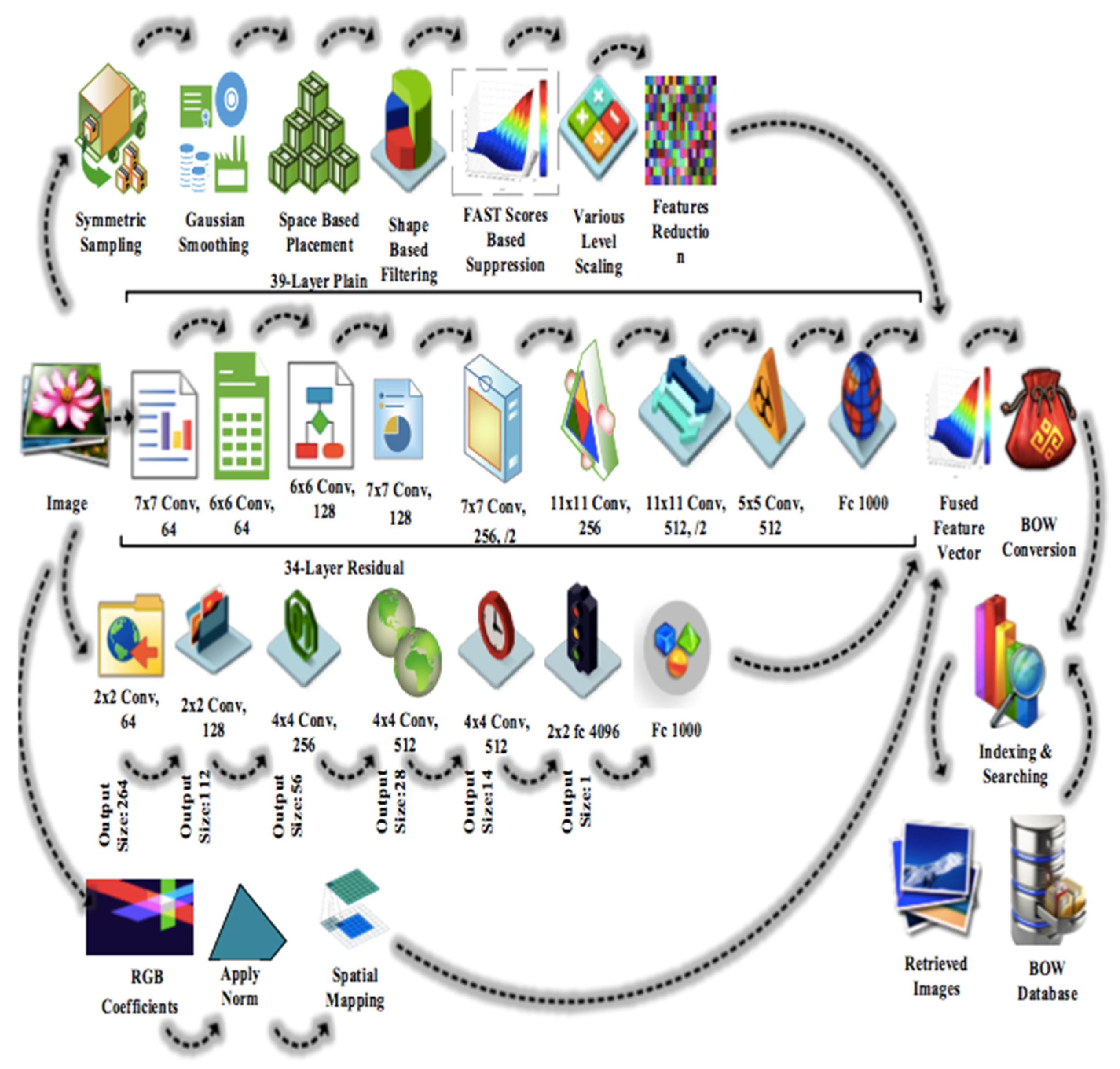
The experimentation was performed on a Core i7 machine (GPU) with 8 GB RAM. MATLAB R2019a provided the testing and training environment with CNN toolbox. Extensive experiments were performed on a variety of datasets to endorse the validity of results.

4.2.1. Results on Large Data

Experiments were performed on large datasets such as Cifar-10 and Cifar-100 to test the effectiveness of the proposed method. The Cifar-10 database contains 60,000 images with 10 different categories of 32 × 32 RGB color images [63]. The Cifar-10 dataset contains various semantic groups such as birds, frogs, ships, dogs, cars, cats, airplanes, horses, deer and trucks. It consists of 6000 images in each category. It is therefore inevitable to produce the retrieval results with the highest throughput. The computational load is an important impact factor at this stage. Our technique adjusted it by applying proper sampling and reduction of features in three stages as follows: first, at symmetry of sampling (Section 3.1) to maintain harmony of samples, secondly at subsampling of features (Section 3.3) and finally by applying principal component analysis (Section 3.7). These three levels of work resulted in prompt feature extraction and quick user response with low computational load. This was endorsed by the statistical fact that aggregate time for feature detection, extraction, fusion, CNN extraction and BoW indexing of an image was ~0.01 to 0.015 s.
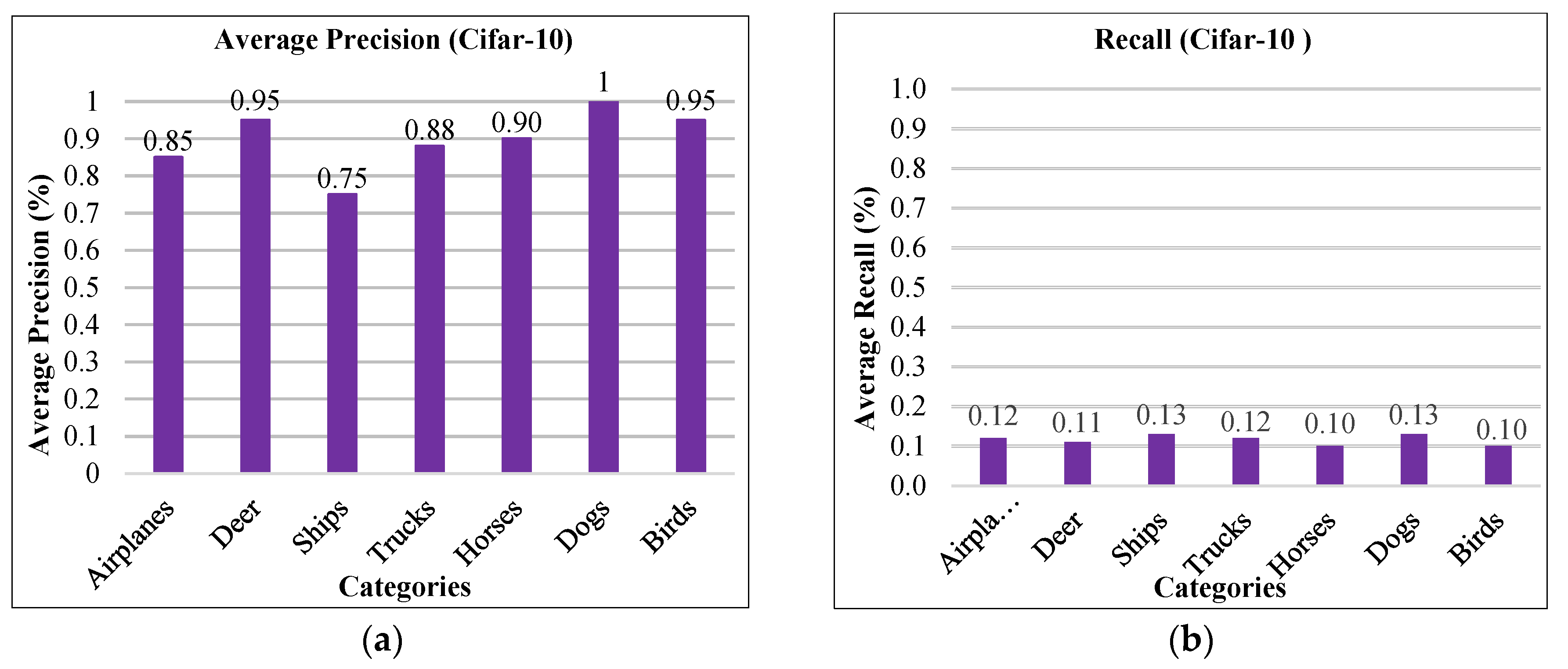
The proposed method showed the highest average precision ratios in seven categories of the Cifar-10 dataset. Figure 2 shows the sample images of different categories in which the proposed method shows the highest average precision rates. The images were classified correctly due to deep learning feature used in the proposed method. Image sampling and scaling integration with CNN features made it possible to correctly classify the images from a large range of image semantic groups, such as airplane, deer, ship, truck, horse, dog and bird. The proposed method provided above 95% mean average precision for these categories. The proposed method also showed better average precision results in some other categories, such as frog, cars and cats. Figure 3 is the graphical representation of average precision (AP) rates in seven categories of the Cifar-10 dataset. Figure 3a reports the highest AP rates in some categories and Figure 3b reports outstanding recall ratio.
The tabular representation of AP rates for the Cifar-10 dataset is shown in Table 1. The proposed method showed above 90% average precision ratio for image categories such as deer, horses, dogs and birds and above 85% average precision results in airplanes and trucks. The category dogs reported a 100% AP rate, which showed the strength of the proposed method. The proposed method showed above 70% AP rates for some other categories. The mAP was 88% in 10 categories of the Cifar-10 dataset.
Figure 4a shows average retrieval precision (ARP) for 10 categories of the Cifar-10 dataset. The proposed method reported the highest ARP ratio for the categories of airplanes and frogs. Other categories also showed above 90% ARP rates, which showed the outstanding performance of the Cifar-10 dataset.
Figure 4b shows the f-measure rate for the proposed method. A pie-chart is used to represent the f-measure. The categories airplanes, frogs, trucks, horses and dogs reported 9% f-measure rate. Other categories showed 11% f-measure rate.
The Cifar-100 dataset is the same as the Cifar-10 dataset with 32 × 32 RGB color images except that it contains 100 different categories. The Cifar-100 dataset contains various semantic groups such as bowls, rabbit, clock, lamp, tiger, forest, mountain, butterfly, elephant, willow, bus, person, house, road, palm, tractor, rocket, motorcycle, etc. It consists of 600 images in each category. The proposed method showed remarkable average precision ratios in most of the Cifar-100 categories. Sample images of Cifar-100 dataset are shown in Figure 5.
The proposed method achieved up to 80% AP in most of the complex image categories of the Cifer-100 dataset, as shown in Table 2. The images were classified well by the presented method. The prosed method used image sampling and shape-based smoothing with a combination of CNN features to classify images of different semantic groups. Different semantic groups of the Cifar-100 dataset include rabbit, whale, trout, flatfish, otter, sunflower, roses, apple, orange, mushroom, bottle, cups, plates, chair, wardrobe, bridge, house, camel, elephant, kangaroo, girl, man, palm, pine, willow, bus, train, rocket, tank, tractor, spider, snail, lizard and turtle. The proposed method reported 100% average precision ratios for many categories, which are mentioned in Table 2. The proposed method showed above 84% mean average precision (mAP) rate for all categories. The proposed method provided significant ARP ratios for most of the categories. The presented technique showed f-measures between 18% and 30% for all categories.
The proposed method reported significant average precision rates for the large size dataset Cifar-100. The proposed method showed excellent performance with 100% average precision rate in most of the categories. It was also observed that the presented method showed more than 80% results in other categories. The strength of the proposed method was its significant average precision results for large datasets such as Cifar-10 and Cifar-100.
The average retrieval precision (ARP) for the Cifar-100 dataset is shown in Figure 6. The proposed method showed outstanding ARP rates for the Cifar-100 dataset. It was observed that above 80% results were achieved in all categories.

4.2.2. Results on Texture Datasets

The ALOT (250) and Fashion (15) datasets are challenging benchmarks for image categorization and classification. These datasets are mainly used to classify texture images from semantic groups. Moreover, the number of categories is an important factor in the domain of content-based image retrieval. For this challenging reason, a large database consisting of 250 categories, the ALOT dataset, was used to test the effectiveness and versatility of the proposed method. The ALOT database [19] contains 250 categories with 100 samples for each. ALOT dataset images have a 384 × 235 pixel resolution [19]. The various semantic groups in the ALOT dataset include fruit, vegetables, clothes, spices, stones, cigarettes, sands, leaves, coins, sea shells, seeds and fabrics, bubbles, embossed fabrics, vertical and horizontal lines, small repeated patterns, etc. These categories contribute different spatial information, objects, object shapes and texture information to classify images. The presented method effectively classified the texture images from semantically similar groups with similar foreground and background objects. Symmetric sampling and norm steps were applied by the proposed method to achieve remarkable results for images with different textures. The images were effectively classified using CNN features with image sampling, scaling integration and shape-based filtering by the proposed method. Scaling on different levels and symmetric sampling were used to achieve significant AP rates for various texture images. In the ALOT dataset, most of the categories contain texture images with similar patterns and colors, whereas other categories contain different object patterns. The presented method showed significant results with up to 80% average precision rates in most of the challenging categories. Sample images for the ALOT dataset with similar colors and similar patterns are shown in Figure 7.
The proposed method showed significant average precision results for images with similar colors and patterns, as shown in Figure 8. It was observed that the texture images in vertical lines with the same color and with different line directions were efficiently classified and showed significant results for different image categories. Gaussian smoothing and shape-based filtering with CNN features made it possible to efficiently classify the texture images from different image categories.
The proposed method showed remarkable average precision ratios in texture images due to Gaussian smoothing and spatial mapping, applied in the presented technique. Most of the categories showed above 80% AP rates, as shown in Figure 8a. Only one category reported 70% AP rate for the proposed method. Figure 8b shows outstanding mean average precision rate for the image categories leaf, stone and fabric. All three categories showed between 90% and 100% mAP rates. Sample images of the ALOT dataset with different color and texture are shown in Figure 9. The RGB coefficient step was used by the proposed method to classify different color images.
Table 3 shows the average precision ratios for the ALOT dataset with different image categories with leaf texture, stone texture, bubble texture, spices texture, sea shells texture, vegetables texture, fruit texture, seeds texture, beans texture, coins texture and fabric texture. It was observed that the proposed method showed above 90% AP rate in most of the bubble texture categories. The proposed method provided outstanding AP ratios in stone texture categories. The category leaf texture also showed significant results with 90% or more AP in most of the categories. Moreover, above 85% AP was achieved in the fabric texture category. The proposed method was also experimentally used for some other categories such as stones, cigarettes, vegetables, beans, coins, spices and fruit. Above 90% results were achieved in most of these categories by the proposed method. Moreover, above 93% mAP was achieved in all categories of the ALOT (250) dataset.
It is noticed that the proposed method showed improved performance for most of the image categories with different shapes and colors. Image sampling, shape-based filtering, RGB coefficients and spatial mapping with CNN features made it possible to effectively and efficiently classify the images. The images were with different categories such as spices, seeds, vegetables and fruit, with different colors. The proposed method showed above 90% results for most of these types of image categories. Similarly, the image categories for embossed fabrics, bubble textures and others were subjected to experiment and classified accurately. Overall, mean average precision was above 93% for all categories of the ALOT (250) dataset.
The versatility and superiority of the proposed method was tested by experimenting with the fashion dataset. The fashion dataset is more suitable for texture analysis, since it contains images with various type of texture, shapes and color objects. The fashion dataset is a challenging set of 15 object categories, which includes 293,800 HD images. The object categories contain different types of fabrics such as uniform, jacket, long dress, shirt, suit, cloak, blouses, sweater, jersey t-shirt, polo-sport shirt, robe, undergarments, vest–waistcoat and coat [64]. In the fashion dataset, there are more than 260 thousand images with different foreground and background textures. The proposed method outperforms for the cluttered and complex objects for the reason of its object recognition capability. The image classification performed remarkably with the proposed method and showed improved AP and AR rates for overlapping, complex and cluttered objects. Figure 10 shows sample images of the fashion dataset.
Figure 11 shows average precision and average recall rates for the fashion dataset. The proposed method was used to experiment with all 15 categories of the fashion dataset. Figure 11a shows the significant results for AP. Three out of 15 categories show 100% AP, whereas other categories also show remarkable results with more than a 70% AP rate. Only one category, vest–waist coat, showed 40% AP rate due to the complex background and fake color images. The proposed method also showed improved results for overlay and complex images, as shown in Figure 11b. The categories coat and uniform reported significant AR rates. The performance of the proposed method was also measured using mean average precision. More than 80% mAP was achieved by the proposed method.
Figure 12a shows ARP for the fashion (15) dataset. The proposed method showed significant ARP rates for the fashion dataset as it used the L2 color coefficient to effectively index and classify the images. Most of the categories, including bloused, jacket, coat, jersey t-shirt, long dress, robe and uniform texture, showed outstanding performance of the proposed method. The ARP rate was above 85% in many categories. The results obtained by f-measure for the fashion dataset are graphically represented in Figure 12b. The proposed method reported encouraging f-measure results. The category vest–waistcoat showed the highest f-measure at 10%. Shirt and Polo-sport shirt reported 8% f-measure, whereas cloak and short dress showed 7% f-measure. All other categories reported 6% f-measure. The significant f- measure results showed the superiority of the presented method for the fashion (15) dataset.

4.2.3. Results on Blobs

The Corel-1000 dataset is commonly used for image classification and retrieval [38,67,68]. Corel datasets consist of various image categories containing plain background images of complex objects. The dataset contains 1000 images in ten categories. The Corel-1000 dataset contains various semantic groups such as food, flowers, animals, natural scenes, buses, buildings, mountains and people. For the object detection and versatility of the image semantics, Corel-1000 was tested. The 100 images had a resolution of 256 × 384 pixels or 384 × 256 pixels for every semantic group. 
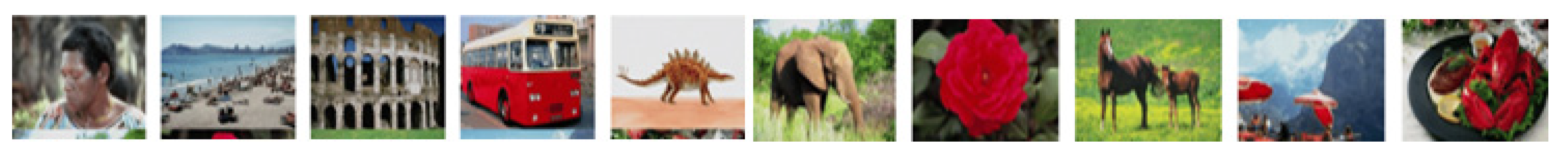
Figure 13 shows sample images of the Corel-1000 dataset.
The average precision results for Corel-1000 dataset are shown in Figure 14a. The proposed method effectively classified the blob images from semantically different groups containing different foreground and background images. The Corel-1000 dataset efficiently classified images due to the deep learning feature of the proposed methods. Image sampling, scaling, integration, shape-based filtering, RGB coefficients and spatial mapping with CNN features made it possible to effectively classify the images. The average precision results for the Corel-1000 dataset show the superiority of the proposed method in blob images due to symmetric sampling, shape-based filtering and RGB coefficient mapping. The proposed method showed significant performance in most of the categories, such as beaches, buildings, buses, dinosaurs, flowers, mountains, horses and food. For complex categories including dinosaurs, flowers and horses, the proposed method reported 100% AP rates. The category buses and mountains showed 97% and 95% AP rate, respectively. Other categories showed above 75% AP rates. The mean average precision for the proposed method was more than 89%. The presented method also showed remarkable results for average recall, as shown in Figure 14b. The categories buses, dinosaurs, flowers and horses reported significant performance with 0.10 AR rate.
The ARP for the Corel-1000 dataset is shown in Figure 15a. The proposed method showed remarkable ARP results for the Corel-1000 dataset. Figure 15b shows f-measure results of the proposed method for Corel-1000 dataset. The categories African, buildings, elephants and food show 11% f-measure, whereas mountains and beaches reported a 10% f-measure, and other categories showed 9% results.

4.2.4. Results for Small and Tiny Images

The Corel 10,000 dataset [19] contains various image categories. The Corel-10000 database is comprised of hundreds of categories where each category contains 100 images. The image size is 128 × 85 pixels or 85 × 128 pixels for every semantic group. The image size of the Corel-10000 dataset is small. The Corel-10000 dataset contains various semantic groups such as butterfly, ketch, cars, planets, flags, texture, shining stars, text, hospital, flowers, food, sunset, animals, human texture and trees etc. Figure 16 is shown sample images of Corel-10000.
Table 4 shows average precision, average recall, ARP and F-measure of the proposed method for the Corel-10000 dataset. The proposed method showed outstanding performance in most of the image categories. The average precision rate was between 70% and 100%. The proposed method showed significant average recall rates. Most of the complex categories reported better performance with 0.10 AR rate. The proposed method showed improved performance for different categories with images of various shape and color. ARP results showed outstanding performance of the proposed method. The proposed method provided above 85% ARP ratios for most of the image categories. The proposed method also showed significant f-measure results for many categories.
The Cifar-100 dataset contains tiny images. The proposed method reported outstanding average precision and f-measure results for tiny and complex images. However, the proposed method provided significant results for tiny images of the Cifar-100 database.

4.2.5. Results of the Corel-1000 Dataset with Existing State-of-the-Art Methods

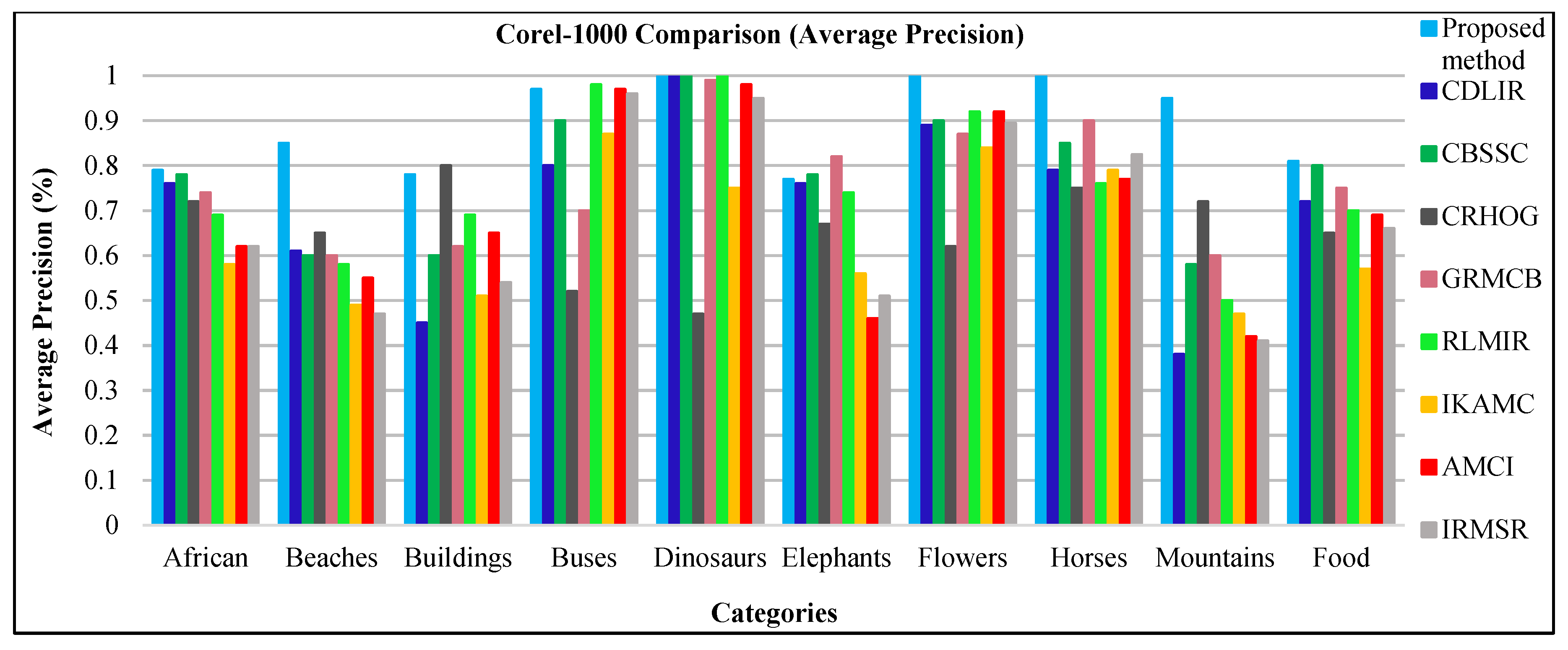
To test the effectiveness and accuracy of the proposed method, the results of the Corel-1000 dataset were compared with the existing state-of-the-art methods. The existing methods include CDLIR [69], CBSSC [70], CRHOG [71], GRMCB [72], RLMIR [73], IKAMC [74], AMCI [75] and IRMSR [76]. A graphical representation of average precision of the proposed method as compared with existing state-of-the-art methods is shown in Figure 17. The proposed method showed outstanding performance in most of the categories, as compared with other methods. The presented method reported the highest average precision rates in the categories African, beaches, dinosaurs, flowers, horses, mountains and food. However, existing state-of-the-art methods showed better average precision results in some categories including buildings, buses and elephants. The proposed method also showed better accuracy in these three categories. RLMIR [73] reported better AP for the category of buses. CRHOG [71] shows improved AP for the category buildings and GRMCB [72] provides better result for the category Elephants.
Table 5 shows the average precision ratio of the proposed method compared with other existing state-of-the-art methods. The performance of the proposed method showed significant average precision rates in African, food, buses, dinosaurs, flowers, horses, mountains and beaches categories. Figure 18 shows the comparison of the proposed method with other existing methods for mean average precision. The proposed method showed highest mAP with 0.89. CBSSC [70] reports second highest mAP as 78%. GRMCB [72] and RLMIR [73] provide mAP as 76%. CDLIR [69], AMCI [75], IRMSR [76] and CRHOG [71] show mAP between 0.66 and 0.76. IKAMC [74] reports lowest mAP as 0.64.

4.2.6. Limitations

The only pitfall to be expected from our approach is that it is not applicable to satellite images.

5. Conclusions

This paper presents a novel technique that detects salient objects, spatial color and texture features in a novel way to represent the image contents accurately and combines them with the signatures extracted by ResNet architecture. The extracted powerful image feature candidates are the information carriers of image contents strengthened by the signatures produced by convolution neural network ResNet. Image smoothing, sampling, suppression and scaling oriented signatures are capable of recognizing the deep image features. The proposed method shows remarkable results on most of the datasets including 250 categories of the ALOT benchmark and 100 categories of Corel-10000. Remarkable results are achieved for the challenging benchmarks including Cifar-100 and Cifar-10. Texture features are finely distinguished by the presented technique at high precision for the fashion dataset. An extension to this contribution is to run it on cloud for VOC.

Author Contributions

Conceptualization, Methodology, Writing, Investigation, Data curation, Formal analysis, Software, implementation, K.K.; Resources, Validation and Supervision, J.L.; Data curation, R.K.; Supervision, K.T.A.; Data curation, A.T.A. All authors have read and agreed to the published version of the manuscript.

Funding

Strategic Priority Research Program of Chinese Academy of Sciences NO. XDA19020102.

Conflicts of Interest

The authors declare no conflict of interest.

References

  1. Guo, J.-M.; Prasetyo, H.; Chen, J.-H. Content-based image retrieval using error diffusion block truncation coding features. IEEE Trans. Circuits Syst. Video Technol. 2015, 25, 466–481. [Google Scholar]
  2. Singh, J.; Bajaj, A.; Mittal, A.; Khanna, A.; Karwayun, R. Content based image retrieval using gabor filters and color coherence vector. In Proceedings of the 2018 IEEE 8th International Advance Computing Conference (IACC), Greater Noida, India, 14–15 December 2018; pp. 290–295. [Google Scholar]
  3. Alhassan, A.K.; Alfaki, A.A. Color and texture fusion-based method for content-based Image Retrieval. In Proceedings of the 2017 International Conference on Communication, Control, Computing and Electronics Engineering (ICCCCEE), Khartoum, Sudan, 16–18 January 2017; pp. 1–6. [Google Scholar]
  4. Dubey, S.R.; Singh, S.K.; Singh, R.K. Boosting local binary pattern with bag-of-filters for content based image retrieval. In Proceedings of the 2015 IEEE UP Section Conference on Electrical Computer and Electronics (UPCON), Allahabad, India, 4–6 December 2015; pp. 1–6. [Google Scholar]
  5. Verma, M.; Raman, B. Local neighborhood difference pattern: A new feature descriptor for natural and texture image retrieval. Multimed. Tools Appl. 2018, 77, 11843–11866. [Google Scholar] [CrossRef]
  6. Saritha, R.R.; Paul, V.; Kumar, P.G. Content based image retrieval using deep learning process. Clust. Comput. 2018, 1–14. [Google Scholar] [CrossRef]
  7. Chen, C.; Zhang, B.; Su, H.; Li, W.; Wang, L. Land-use scene classification using multi-scale completed local binary patterns. Signal Image Video Process. 2016, 10, 745–752. [Google Scholar] [CrossRef]
  8. Nogueira, K.; Penatti, O.A.; dos Santos, J.A. Towards better exploiting convolutional neural networks for remote sensing scene classification. Pattern Recognit. 2017, 61, 539–556. [Google Scholar] [CrossRef] [Green Version]
  9. Bringer, J.; Chabanne, H.; Patey, A. Privacy-preserving biometric identification using secure multiparty computation: An overview and recent trends. IEEE Signal Process. Mag. 2013, 30, 42–52. [Google Scholar] [CrossRef]
  10. Sharma, K.U.; Thakur, N.V. A review and an approach for object detection in images. Int. J. Comput. Vis. Robot. 2017, 7, 196–237. [Google Scholar] [CrossRef]
  11. Jia, H.; Ding, S.; Xu, X.; Nie, R. The latest research progress on spectral clustering. Neural Comput. Appl. 2014, 24, 1477–1486. [Google Scholar] [CrossRef]
  12. Luo, J.; Joshi, D.; Yu, J.; Gallagher, A. Geotagging in multimedia and computer vision—A survey. Multimed. Tools Appl. 2011, 51, 187–211. [Google Scholar] [CrossRef]
  13. Maind, S.B.; Wankar, P. Research paper on basic of artificial neural network. Int. J. Recent Innov. Trends Comput. Commun. 2014, 2, 96–100. [Google Scholar]
  14. Chang, F.-A.; Tsai, C.-C.; Tseng, C.-K.; Guo, J.-I. Embedded multiple object detection based on deep learning technique for advanced driver assistance system. In Proceedings of the 2017 IEEE 60th International Midwest Symposium on Circuits and Systems (MWSCAS), Boston, MA, USA, 6–9 August 2017; pp. 172–175. [Google Scholar]
  15. Deng, F.; Zhu, X.; Ren, J. Object detection on panoramic images based on deep learning. In Proceedings of the 2017 3rd International Conference on Control, Automation and Robotics (ICCAR), Nagoya, Japan, 24–26 April 2017; pp. 375–380. [Google Scholar]
  16. Tian, B.; Li, L.; Qu, Y.; Yan, L. Video object detection for tractability with deep learning method. In Proceedings of the 2017 Fifth International Conference on Advanced Cloud and Big Data (CBD), Shanghai, China, 13–16 August 2017; pp. 397–401. [Google Scholar]
  17. Ahmed, K.T.; Iqbal, M.A. Region and texture based effective image extraction. Clust. Comput. 2018, 21, 493–502. [Google Scholar] [CrossRef]
  18. Ahmed, K.T.; Irtaza, A.; Iqbal, M.A. Fusion of local and global features for effective image extraction. Appl. Intell. 2017, 47, 526–543. [Google Scholar] [CrossRef]
  19. Ahmed, K.T.; Ummesafi, S.; Iqbal, A. Content based image retrieval using image features information fusion. Inf. Fusion 2019, 51, 76–99. [Google Scholar] [CrossRef]
  20. Diba, A.; Sharma, V.; Pazandeh, A.; Pirsiavash, H.; Van Gool, L. Weakly supervised cascaded convolutional networks. In Proceedings of the IEEE Conference on Computer Vision and Pattern Recognition, Honolulu, HI, USA, 21–26 July 2017; pp. 914–922. [Google Scholar]
  21. Ouyang, W.; Zeng, X.; Wang, X.; Qiu, S.; Luo, P.; Tian, Y.; Li, H.; Yang, S.; Wang, Z.; Li, H. DeepID-Net: Object detection with deformable part based convolutional neural networks. IEEE Trans. Pattern Anal. Mach. Intell. 2017, 39, 1320–1334. [Google Scholar] [CrossRef] [PubMed]
  22. Chen, X.; Yuille, A.L. Articulated pose estimation by a graphical model with image dependent pairwise relations. In Proceedings of the Advances in Neural Information Processing Systems, Montreal, OC, Cananda, 8 December 2014; pp. 1736–1744. [Google Scholar]
  23. Toshev, A.; Szegedy, C. Deeppose: Human pose estimation via deep neural networks. In Proceedings of the IEEE Conference on Computer Vision and Pattern Recognition, Columbus, OH, USA, 23–28 June 2014; pp. 1653–1660. [Google Scholar]
  24. Doulamis, N. Adaptable deep learning structures for object labeling/tracking under dynamic visual environments. Multimed. Tools Appl. 2018, 77, 9651–9689. [Google Scholar] [CrossRef]
  25. Doulamis, N.; Voulodimos, A. FAST-MDL: Fast adaptive supervised training of multi-layered deep learning models for consistent object tracking and classification. In Proceedings of the 2016 IEEE International Conference on Imaging Systems and Techniques (IST), Chania, Greece, 4–6 October 2016; pp. 318–323. [Google Scholar]
  26. Long, J.; Shelhamer, E.; Darrell, T. Fully convolutional networks for semantic segmentation. In Proceedings of the IEEE Conference on Computer Vision and Pattern Recognition, Boston, MA, USA, 7–12 June 2015; pp. 3431–3440. [Google Scholar]
  27. Noh, H.; Hong, S.; Han, B. Learning deconvolution network for semantic segmentation. In Proceedings of the IEEE International Conference on Computer Vision, Boston, MA, USA, 7–12 June 2015; pp. 1520–1528. [Google Scholar]
  28. Cao, S.; Nevatia, R. Exploring deep learning based solutions in fine grained activity recognition in the wild. In Proceedings of the 2016 23rd International Conference on Pattern Recognition (ICPR), Cancun, Mexico, 4–8 December 2016; pp. 384–389. [Google Scholar]
  29. Lin, L.; Wang, K.; Zuo, W.; Wang, M.; Luo, J.; Zhang, L. A deep structured model with radius–margin bound for 3D human activity recognition. Int. J. Comput. Vis. 2016, 118, 256–273. [Google Scholar] [CrossRef] [Green Version]
  30. Hinton, G.E.; Salakhutdinov, R.R. A better way to pretrain deep boltzmann machines. In Proceedings of the Advances in Neural Information Processing Systems, Lake Tahoe, NV, USA, 3–6 December 2012; pp. 2447–2455. [Google Scholar]
  31. Salakhutdinov, R.; Hinton, G. Deep boltzmann machines. In Proceedings of the Artificial intelligence and Statistics (AISTATS), Clearwa-ter Beach, FL, USA, 16–18 April 2009; pp. 448–455. [Google Scholar]
  32. Ouyang, Y.; Liu, W.; Rong, W.; Xiong, Z. Autoencoder-based collaborative filtering. In Proceedings of the International Conference on Neural Information Processing, Kuching, Malaysia, 3–6 November 2014; pp. 284–291. [Google Scholar]
  33. Dubey, S.R.; Singh, S.K.; Singh, R.K. Rotation and illumination invariant interleaved intensity order-based local descriptor. IEEE Trans. 2014, 23, 5323–5333. [Google Scholar] [CrossRef]
  34. Ramesh, B.; Xiang, C.; Lee, T.H. Shape classification using invariant features and contextual information in the bag-of-words model. Pattern Recognit. 2015, 48, 894–906. [Google Scholar] [CrossRef]
  35. Long, D.F.; Zhang, D.H.; Feng, D.D. Fundamentals of content based image retrieval. Second Int. Educ. Technol. Comput. Sci. 2008. [Google Scholar] [CrossRef]
  36. Lu, T.-C.; Chang, C.-C. Color image retrieval technique based on color features and image bitmap. Inf. Process. Manag. 2007, 43, 461–472. [Google Scholar] [CrossRef]
  37. Shen, G.-L.; Wu, X.-J. Content based image retrieval by combining color, texture and CENTRIST. In Proceedings of the 2013 Constantinides International Workshop on Signal Processing (CIWSP 2013), London, UK, 25–25 January 2013. [Google Scholar]
  38. Shrivastava, N.; Tyagi, V. An efficient technique for retrieval of color images in large databases. Comput. Electr. Eng. August 2015, 46, 314–327. [Google Scholar] [CrossRef]
  39. Benitez, A.B.; Beigi, M.; Chang, S.-F. Using relevance feedback in content-based image metasearch. IEEE Internet Comput. 1998, 2, 59–69. [Google Scholar] [CrossRef]
  40. Lew, M.S.; Sebe, N.; Djeraba, C.; Jain, R. Content-based multimedia information retrieval: State of the art and challenges. ACM Trans. Multimed. Comput. Commun. Appl. 2006, 2, 1–19. [Google Scholar] [CrossRef]
  41. Smeulders, A.W.; Worring, M.; Santini, S.; Gupta, A.; Jain, R. Content-based image retrieval at the end of the early years. IEEE Trans. Pattern Anal.Mach. Intell. 2000, 22, 1349–1380. [Google Scholar] [CrossRef]
  42. Sadeghi, A.-R.; Schneider, T.; Wehrenberg, I. Efficient privacypreserving face recognition. In Proceedings of the 12th International Conference on Information Security and Cryptology (ICISC), Seoul, Korea, 2–4 December 2009; pp. 229–244. [Google Scholar]
  43. Ackley, D.H.; Hinton, G.E.; Sejnowski, T.J. A learning algorithm for Boltzmann machines. Cogn. Sci. 1985, 9, 147–169. [Google Scholar] [CrossRef]
  44. Hinton, G.; Deng, L.; Yu, D.; Dahl, G.; Mohamed, A.-R.; Jaitly, N.; Senior, A.; Vanhoucke, V.; Nguyen, P.; Kingsbury, B. Deep neural networks for acoustic modeling in speech recognition. IEEE Signal Process. Mag. 2012, 29. [Google Scholar] [CrossRef]
  45. Hinton, G.E.; Osindero, S.; Teh, Y.-W. A fast learning algorithm for deep belief nets. Neural Comput. 2006, 18, 1527–1554. [Google Scholar] [CrossRef]
  46. Salakhutdinov, R.; Mnih, A.; Hinton, G. Restricted Boltzmann machines for collaborative filtering. In Proceedings of the 24th International Conference on Machine Learning, Corvolis, OR, USA, 20–24 June 2007; pp. 791–798. [Google Scholar]
  47. Alzu’bi, A.; Amira, A.; Ramzan, N. Content-based image retrieval with compact deep convolutional features. Neurocomputing 2017, 249, 95–105. [Google Scholar] [CrossRef] [Green Version]
  48. Babenko, A.; Slesarev, A.; Chigorin, A.; Lempitsky, V. Neural codes for image retrieval. In Proceedings of the European Conference on Computer Vision, Zurich, Switzerland, 6–12 September 2014; pp. 584–599. [Google Scholar]
  49. Tolias, G.; Sicre, R.; Jégou, H. Particular object retrieval with integral max-pooling of CNN activations. Comput. Vis. Pattern Recognit. arXiv 2015, arXiv:1511.05879. [Google Scholar]
  50. Mohedano, E.; McGuinness, K.; O’Connor, N.E.; Salvador, A.; Marques, F.; Giro-i-Nieto, X. Bags of local convolutional features for scalable instance search. In Proceedings of the ACM on International Conference on Multimedia Retrieval, New York, NY, USA, 6–9 June 2016; pp. 327–331. [Google Scholar]
  51. Yu, W.; Yang, K.; Yao, H.; Sun, X.; Xu, P. Exploiting the complementary strengths of multi-layer CNN features for image retrieval. Neurocomputing 2017, 237, 235–241. [Google Scholar] [CrossRef]
  52. Lin, T.-Y.; RoyChowdhury, A.; Maji, S. Bilinear cnn models for fine-grained visual recognition. In Proceedings of the IEEE International Conference on Computer Vision, Boston, MA, USA, 7–12 June 2015; pp. 1449–1457. [Google Scholar]
  53. Ma, X.; Wang, J. Image retrieval using deep convolutional neural networks and regularized locality preserving indexing strategy. J. Comput. Commun. 2017, 5, 33. [Google Scholar] [CrossRef] [Green Version]
  54. Wei, Q.; Wang, W. Research on image retrieval using deep convolutional neural network combining L1 regularization and PRelu activation function. In Proceedings of the IOP Conference Series: Earth and Environmental Science, Chengdu, China, 26–28 May 2017; p. 012156. [Google Scholar]
  55. Calonder, M.; Lepetit, V.; Strecha, C.; Fua, P. Brief: Binary robust independent elementary features. In Proceedings of the European Conference on Computer Vision, Heraklion, Crete, Greece, 5–11 September 2010; pp. 778–792. [Google Scholar]
  56. Leutenegger, S.; Chli, M.; Siegwart, R. BRISK: Binary robust invariant scalable keypoints. In Proceedings of the IEEE International Conference on Computer Vision (ICCV), Barcelona, Spain, 6–13 November 2011; pp. 2548–2555. [Google Scholar]
  57. Bay, H.; Tuytelaars, T.; Van Gool, L. Surf: Speeded up robust features. In Proceedings of the European Conference on Computer Vision, Graz, Austria, 7–13 May 2006; pp. 404–417. [Google Scholar]
  58. Viswanathan, D.G. Features from accelerated segment test (FAST). In Proceedings of the 10th workshop on Image Analysis for Multimedia Interactive Services, London, UK, 6–8 May 2009. [Google Scholar]
  59. Lindeberg, T. Scale-Space: A Framework for Handling Image Structures at Multiple Scales; KTH, S-100 44; CERN: Stockholm, Sweden, 1996. [Google Scholar]
  60. Burghouts, G.J.; Geusebroek, J.-M. Material-specific adaptation of color invariant features. Pattern Recognit. Lett. 2009, 30, 306–313. [Google Scholar] [CrossRef]
  61. Constantin, C. Principal component analysis-a powerful tool in computing marketing information. Bull. Transilv. Univ. Brasov. Econ. Sci. Ser. V 2014, 7, 25. [Google Scholar]
  62. He, K.; Zhang, X.; Ren, S.; Sun, J. Deep residual learning for image recognition. In Proceedings of the IEEE Conference on Computer Vision and Pattern Recognition, Las Vegas, NV, USA, 26 June–July 1 2016; pp. 770–778. [Google Scholar]
  63. Zhu, X.; Bain, M. B-CNN: Branch convolutional neural network for hierarchical classification. Comput. Vis. Pattern Recognit. arXiv 2017, arXiv:1709.09890. [Google Scholar]
  64. Rostamzadeh, N.; Hosseini, S.; Boquet, T.; Stokowiec, W.; Zhang, Y.; Jauvin, C.; Pal, C. Fashion-gen: The generative fashion dataset and challenge. Mach. Learn. arXiv 2018, arXiv:1806.08317. [Google Scholar]
  65. Steger, C. Occlusion, clutter, and illumination invariant object recognition. Int. Arch. Photogramm. Remote Sens. Spat. Inf. Sci. 2002, 34, 345–350. [Google Scholar]
  66. Kandefer, M.; Shapiro, S. An F-measure for context-based information retrieval. Commonsense 2009, 79–84. [Google Scholar]
  67. Dubey, S.R.; Singh, S.K.; Singh, R.K. Multichannel decoded local binary patterns for content-based image retrieval. IEEE Trans. Image Process. 2016, 25, 4018–4032. [Google Scholar] [CrossRef]
  68. Zhou, Y.; Zeng, F.-Z.; Zhao, H.-M.; Murray, P.; Ren, J. Hierarchical visual perception and two-dimensional compressive sensing for effective content-based color image retrieval. Cogn. Comput. 2016, 8, 877–889. [Google Scholar] [CrossRef] [Green Version]
  69. Garg, M.; Malhotra, M.; Singh, H. Comparison of deep learning techniques on content based image retrieval. Mod. Phys. Lett. A 2019, 1950285. [Google Scholar] [CrossRef]
  70. Jin, C.; Ke, S.-W. Content-based image retrieval based on shape similarity calculation. 3D Res. 2017, 8, 23. [Google Scholar] [CrossRef]
  71. Pan, S.; Sun, S.; Yang, L.; Duan, F.; Guan, A. Content retrieval algorithm based on improved HOG. In Proceedings of the 2015 3rd International Conference on Applied Computing and Information Technology/2nd International Conference on Computational Science and Intelligence, Okayama, Japan, 12–16 July 2015; pp. 438–441. [Google Scholar]
  72. Kundu, M.K.; Chowdhury, M.; Bulò, S.R. A graph-based relevance feedback mechanism in content-based image retrieval. Knowl.-Based Syst. 2015, 73, 254–264. [Google Scholar] [CrossRef]
  73. Memon, M.H.; Li, J.; Memon, I.; Arain, Q.A.; Memon, M.H. Region based localized matching image retrieval system using color-size features for image retrieval. In Proceedings of the 2017 14th International Computer Conference on Wavelet Active Media Technology and Information Processing (ICCWAMTIP), Chengdu, China, 15–17 December 2017; pp. 211–215. [Google Scholar]
  74. Sejal1, D.; Rashmi1, V.; Venugopal1, K.R.; Iyengar, S.S.; Patnaik, L.M. Image recommendation based on keyword relevance usingabsorbing Markov chain and image features. Int. J. Multimed. Info. Retr. 2016, 5, 185–199. [Google Scholar] [CrossRef] [Green Version]
  75. Zheng, L.; Wang, S.; Wang, J.; Tian, Q. Accurate image search with multi-scale contextual evidences. Int. J. Comput. Vis. 2016, 120, 1–13. [Google Scholar] [CrossRef]
  76. Zeng, Z.; Song, L.; Zheng, Q.; Chi, Y. A new image retrieval model based on monogenic signal representation. J. Vis. Commun. Image Represent. 2015, 33, 85–93. [Google Scholar] [CrossRef]
Figure 1. The proposed method is showing the step-by-step objects detection process.
Symmetry 12 00612 g001
Figure 2. Cifar-10 dataset showing different sample images from 10 categories [63].
Symmetry 12 00612 g002
Figure 3. (a) Graphical illustration of the average precision on Cifar-10 dataset; (b) Average recall on Cifar-10 dataset.
Symmetry 12 00612 g003
Figure 4. (a) Graphical illustration of the average retrieval precision on Cifar-10 dataset; (b) F-measure on Cifar-10 dataset.
Symmetry 12 00612 g004
Figure 5. Cifar-100 dataset showing different sample images from 100 categories [63].
Symmetry 12 00612 g005
Figure 6. Graphical illustration of the average retrieval precision on Cifar-100 dataset.
Symmetry 12 00612 g006
Figure 7. ALOT dataset showing sample images with almost the same colors and pattern [19].
Symmetry 12 00612 g007
Figure 8. (a) Graphical illustration of the average precision on ALOT dataset with similar colors and patterns; (b) Graphical representation of the mean average precision (category-wise) on ALOT (250) dataset for stone texture, spice texture and fabric texture.
Symmetry 12 00612 g008
Figure 9. A LOT (250) dataset showing sample images with leaf texture, stone texture and fabric texture [19].
Symmetry 12 00612 g009
Figure 10. Fashion (15) dataset showing sample images from different categories [64].
Symmetry 12 00612 g010
Figure 11. (a) Graphical illustration of the average recall on the fashion dataset; (b) Average recall on the fashion dataset.
Symmetry 12 00612 g011
Figure 12. (a) Graphical illustration of the average retrieval precision on the fashion (15) dataset; (b) Graphical illustration of F-measure on the fashion (15) dataset.
Symmetry 12 00612 g012
Figure 13. Corel-1000 dataset: Sample images from each category [19].
Symmetry 12 00612 g013
Figure 14. (a) Graphical illustration of the average precision on Corel-1000 dataset; (b) Average recall on Corel-1000 dataset.
Symmetry 12 00612 g014
Figure 15. (a) Graphical illustration of the average retrieval precision on Corel-1000 dataset; (b) Graphical illustration of F-measure on Corel-1000 dataset.
Symmetry 12 00612 g015
Figure 16. Corel-10000 dataset: Sample images from some categories [19].
Symmetry 12 00612 g016
Figure 17. Comparison of the average precisions attained by the proposed method and other standard retrieval systems using the Corel-1000 dataset.
Symmetry 12 00612 g017
Figure 18. Graphical representation of the mean average precision on Corel-1000 dataset with existing state of art methods.
Symmetry 12 00612 g018
Table 1. The highest average precision ratios of the proposed method in Cifar-10 dataset.
Cifar-10 Dataset—Average Precision
CategoriesAirplanesDeerShipsTrucksHorsesDogsBirds
Average Precision0.850.950.750.880.9010.95
Table 2. The average precision, recall, ARP and F-Measure of Cifar-100.
Cifar-100 Dataset (Precision, Recall, ARP and F-Measure)
CategoryPrecisionRecallARPF-MeasureCategoryPrecisionRecallARPF-Measure
11.000.101.000.18510.900.110.850.20
21.000.101.000.18520.800.130.850.22
30.650.150.880.25530.850.120.900.21
41.000.100.910.18541.000.100.850.18
50.900.110.910.20550.900.110.850.20
60.800.130.890.22560.600.170.870.26
70.900.110.890.20570.950.110.850.19
80.950.110.900.19580.700.140.860.24
91.000.100.910.18591.000.100.880.18
100.850.120.900.21600.900.110.880.20
110.950.110.910.19610.950.110.870.19
120.500.200.880.29620.950.110.870.19
130.800.130.870.22630.900.110.850.20
140.850.120.870.21640.700.140.870.24
150.850.120.870.21650.500.200.820.29
160.900.110.870.20660.400.250.760.31
171.000.100.880.18670.650.150.840.25
180.700.140.870.24680.950.110.830.19
190.800.130.860.22690.950.110.820.19
200.800.130.860.22701.000.100.840.18
210.900.110.860.20710.800.130.840.22
221.000.100.870.18720.850.120.840.21
230.950.110.870.19730.300.330.810.32
241.000.100.880.18740.900.110.830.20
250.800.130.870.22750.500.200.730.29
260.700.140.870.24760.900.110.760.20
270.550.180.860.27770.750.130.730.23
280.550.180.840.27780.700.140.700.24
290.950.110.850.19790.950.110.800.19
300.550.180.800.27800.750.130.730.23
310.750.130.790.23810.900.110.750.20
320.800.130.820.22820.600.170.780.26
330.850.120.820.21831.000.100.820.18
340.950.110.840.19840.950.110.770.19
351.000.100.840.18850.750.130.830.23
360.850.120.830.21861.000.100.820.18
371.000.100.850.18870.900.110.810.20
380.900.110.820.20880.850.120.800.21
390.550.180.850.27890.600.170.860.26
401.000.100.850.18900.800.130.820.22
410.600.170.790.26911.000.100.810.18
421.000.100.830.18920.950.110.820.19
431.000.100.840.18930.500.200.800.29
440.950.110.840.19941.000.100.830.18
450.750.130.820.23950.900.110.800.20
460.900.110.830.20960.950.110.830.19
471.000.100.840.18971.000.100.810.18
480.750.130.880.23980.950.110.800.19
491.000.100.850.18991.000.100.830.18
500.950.110.850.191000.950.110.850.19
Table 3. The average precision ratios of the proposed method for ALOT (250) dataset.
ALOT Dataset (Average Precision)
Bubble Textures
CategoryPrecisionCategoryPrecisionCategoryPrecisionCategoryPrecision
11.0071.00130.98191.00
21.0080.97140.91200.85
30.9890.95151.00210.89
40.97100.96160.90220.70
50.95111.00171.00
60.85120.92180.88
Stone Textures
CategoryPrecisionCategoryPrecisionCategoryPrecisionCategoryPrecision
10.8580.87151.00220.90
21.0091.00160.96230.86
30.80100.86171.00241.00
40.90111.00180.92250.88
50.90120.94191.00261.00
61.00130.92201.00
71.00140.98211.00
Leaf Textures
CategoryPrecisionCategoryPrecisionCategoryPrecisionCategoryPrecision
10.9380.98150.91220.91
20.9690.87160.88230.96
31.00100.92170.90240.98
40.95110.97180.87251.00
50.86120.96191.00261.00
60.90131.00201.00270.90
70.90141.00210.90280.96
Fabric Textures
CategoryPrecisionCategoryPrecisionCategoryPrecisionCategoryPrecision
10.98101.00190.98280.96
20.94110.92201.00290.86
30.80120.98210.75300.88
40.89130.96221.00310.92
50.86140.94230.98320.98
60.92151.00240.95330.97
71.00161.00251.00340.94
81.00170.85260.98351.00
90.98180.95270.94
Vegetable Textures
CategoryPrecisionCategoryPrecisionCategoryPrecisionCategoryPrecision
10.9840.9270.8101.00
20.8850.9881.00111.00
30.9061.0090.65120.96
Fruit Textures
CategoryPrecisionCategoryPrecisionCategoryPrecisionCategoryPrecision
10.9260.97110.89160.89
20.9070.94120.93171.00
30.8880.92130.96180.95
40.8691.00140.95190.75
50.98101.00150.97201.00
Seed Textures
CategoryPrecisionCategoryPrecisionCategoryPrecisionCategoryPrecision
11.0050.9590.92130.70
20.9660.8100.95140.89
30.9271.00110.98150.87
41.0081.00120.95
Bean Textures
CategoryPrecisionCategoryPrecisionCategoryPrecisionCategoryPrecision
10.9050.6090.50131.00
21.0060.90101.00140.80
30.7570.95110.85151.00
41.0080.98121.00
Coin Textures
CategoryPrecisionCategoryPrecisionCategoryPrecisionCategoryPrecision
10.9470.87131.00190.89
20.9880.95140.98200.90
30.9591.00150.96211.00
40.94101.00160.86221.00
50.98110.90170.89
60.89121.00180.98
Sea Shell Textures
CategoryPrecisionCategoryPrecisionCategoryPrecisionCategoryPrecision
10.9661.00110.95161.00
20.9270.98120.96170.86
31.0080.96130.98180.98
40.8090.89141.00190.97
50.98100.91150.55200.92
Spice Textures
CategoryPrecisionCategoryPrecisionCategoryPrecisionCategoryPrecision
10.90100.86190.88281.00
20.75110.85200.86290.95
30.75120.95210.98300.93
41.00130.95220.94310.91
50.60140.98230.92321.00
60.88150.89241.00330.88
70.95160.85251.00340.80
81.00170.98260.89350.70
90.94180.94270.96
Table 4. The average precision, recall, ARP and F-measure of Corel-10000.
Corel-10000 Dataset (Precision, Recall, ARP and F-Measure)
CategoryPrecisionRecallARPF-MeasureCategoryPrecisionRecallARPF-Measure
11.000.1010.18510.800.130.900.22
20.700.140.850.24521.000.100.900.18
31.000.100.900.18530.850.120.900.21
40.850.120.890.21541.000.100.900.18
50.750.130.860.23550.800.130.900.22
61.000.100.880.18561.000.100.900.18
71.000.100.900.18571.000.100.900.18
80.900.110.900.20580.950.110.900.19
90.900.110.900.20590.900.110.900.20
100.800.130.890.22601.000.100.900.18
110.850.120.890.21610.800.130.900.22
121.000.100.900.18621.000.100.900.18
130.950.110.900.19630.900.110.900.20
140.650.150.880.256420.000.100.900.18
150.800.130.880.22650.950.110.900.19
160.700.140.870.24661.000.100.910.18
170.700.140.860.24670.950.110.910.19
180.900.110.860.20680.900.110.910.20
191.000.100.870.18691.000.100.910.18
201.000.100.870.18700.850.120.910.21
210.800.130.870.22711.000.100.910.18
221.000.100.880.18720.850.120.910.21
230.800.130.870.22730.950.110.910.19
241.000.100.880.18741.000.100.910.18
250.900.110.880.20750.950.110.910.19
260.800.130.880.22760.900.110.910.20
270.850.120.870.21771.000.100.910.18
280.800.130.870.22780.850.120.910.21
291.000.100.880.18790.900.110.910.20
301.000.100.880.18801.000.100.910.18
310.750.130.880.23810.700.140.910.24
321.000.100.880.18821.000.100.910.18
331.000.100.880.18831.000.100.910.18
340.800.130.880.22840.800.130.910.22
350.950.110.880.19851.000.100.910.18
361.000.100.890.18860.950.110.910.19
370.850.120.890.21871.000.100.910.18
380.900.110.890.20881.000.100.910.18
390.900.110.890.20891.000.100.910.18
401.000.100.890.18901.000.100.920.18
410.800.130.890.22910.800.130.910.22
420.900.110.890.20920.800.130.910.22
431.000.100.890.18931.000.100.910.18
441.000.100.890.18940.850.120.910.21
451.000.100.890.18951.000.100.910.18
461.000.100.900.18960.950.110.910.19
471.000.100.900.18970.900.110.910.20
481.000.100.900.18981.000.100.910.18
490.900.110.900.20990.950.110.920.19
500.700.140.900.241001.000.100.920.18
Table 5. Comparison of the average precision of the proposed method in comparison with the existing research methods.
Corel-1000 Dataset vs. Existing Methods—Average Precision
ClassProposed MethodCDLIR [69]CBSSC [70]CRHOG [71]GRMCB [72]RLMIR [73]IKAMC [74]AMCI [75]IRMSR [76]
African0.790.760.780.720.740.690.580.620.62
Beaches0.850.610.600.650.600.580.490.550.47
Buildings0.780.450.600.800.620.690.510.650.54
Buses0.970.800.900.520.700.980.870.970.96
Dinosaurs1.001.001.000.470.991.000.750.980.95
Elephants0.770.760.780.670.820.740.560.460.51
Flowers1.000.890.900.620.870.920.840.920.89
Horses1.000.790.850.750.900.760.790.770.82
Mountains0.950.380.580.720.600.500.470.420.41
Food0.810.720.800.650.750.700.570.690.66
Average0.890.720.780.670.750.760.640.700.69

