Symmetry Evolution in Chaotic System

Abstract

A comprehensive exploration of symmetry and conditional symmetry is made from the evolution of symmetry. Unlike other chaotic systems of conditional symmetry, in this work it is derived from the symmetric diffusionless Lorenz system. Transformation from symmetry and asymmetry to conditional symmetry is examined by constant planting and dimension growth, which proves that the offset boosting of some necessary variables is the key factor for reestablishing polarity balance in a dynamical system.

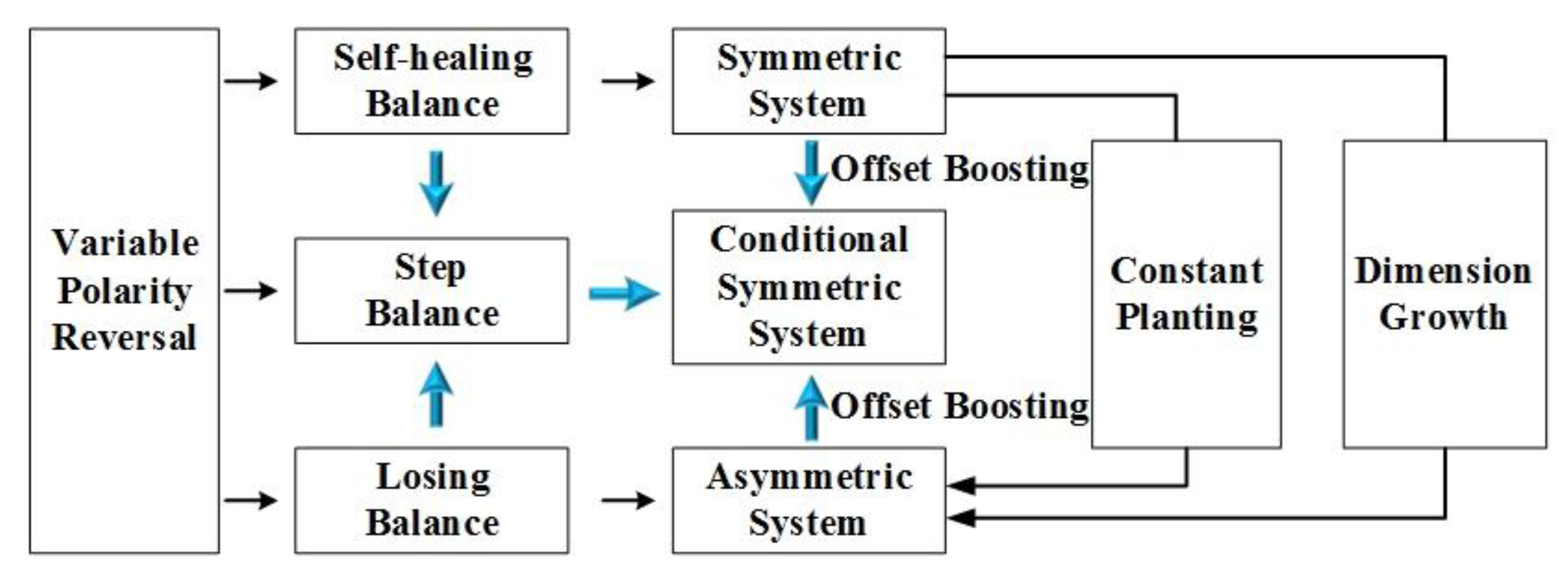
1. Introduction

The system structure is a fundamental topological constraint to the dynamical evolution, which determines how the attractor stretches in phase space. Symmetric systems give birth to attractors with a symmetrical face [1,2,3,4,5]. When symmetry is broken, the attractor splits into a symmetric pair of attractors [6,7,8] or is preserved by doubling coexisting attractors [9]. Asymmetric systems seem to give a single asymmetric attractor in most cases, although sometimes it hatches coexisting asymmetric attractors [10,11,12,13,14] under a set of combined parameters. However, many asymmetric systems have coexisting attractors of conditional symmetry with the new polarity balance from the offset boosting.

Furthermore, symmetric structure does not reject conditional symmetry. In this paper, the symmetry evolution in chaotic systems is analyzed, as shown in Figure 1. From the start of the variable polarity reversal, if a dynamical system can establish its own polarity balance from itself, the system is symmetric, or else losing the polarity balance indicates the asymmetric structure. If a system recovers its polarity balance from a step with offset boosting, the derived system is of conditional symmetry. From this observation, we can conclude that a system, whether it is symmetric or asymmetric, can be transformed to be of conditional symmetry. In Section 2, the early proposed chaotic systems of conditional symmetry are collected. In Section 3, conditional symmetry is coined in a symmetric system. In Section 4, the collapse of polarity balance is thoroughly explored in two directions, one of which is from the constant planting, and the other of which is from the dimension growth. Conditional symmetry is therefore in the primary road where the offset-boosting-induced polarity balance is well preserved. The conclusion is given in the last section.

2. Conditional Symmetry from Asymmetry

As we know, for a dynamical system $\dot{X}=F\left(X\right)={\left(f_1\left(X\right),f_2\left(X\right),\dots ,f_N\left(X\right)\right)}^T$, ($X={\left(x_1,x_2,\dots ,x_N\right)}^T)$, if there exists a variable substitution $u_{i_1}=-x_{i_1},u_{i_2}=-x_{i_2},\cdots ,u_{i_k}=-x_{i_k},u_i=x_i$, (here $1\le i_1,\cdots ,i_k\le N,i_1,\cdots ,i_k$ are not identical, $i\in \left\{1,2,\dots ,N\right\}\backslash \left\{i_1,\cdots ,i_k\right\}$) satisfying $\dot{U}=F\left(U\right)$ ($U=\left(u_1,u_2,\dots ,u_N\right))$, then the system $\dot{X}=F\left(X\right)$ ($X=\left(x_1,x_2,\dots ,x_N\right))$ is symmetric. Conditional symmetry is a new terminology to describe the polarity balance from offset boosting [15,16,17,18]. For a differential dynamical system, $\dot{X}=F\left(X\right)=$ ${\left(f_1\left(X\right),f_2\left(X\right),\dots ,f_N\left(X\right)\right)}^T$, ($X={\left(x_1,x_2,\dots ,x_N\right)}^T)$, the substitution $u_{i_0}=x_{i_0}+c$ ($i_0\in \left\{1,2,\dots ,N\right\}$ (c is an arbitrary constant) brings the offset boosting in the variable $x_{i_0}$, where the new constant c will change the average value of the variable $x_{i_0}$. For a dynamical system, if there exists a variable substitution, $u_{i_0}=x_{i_0}+c_0$, $u_i=x_i$ (here $c_0$ is a non-zero constant, then $i_0\in \left\{1,2,\dots ,N\right\},$ and $i\in \left\{1,2,\dots ,N\right\}\backslash \left\{i_0\right\}$), which makes the deduced system $\dot{U}=F^{*}\left(U\right)=\left(f_1^{*}\left(U\right),f_2^{*}\left(U\right),\dots ,f_N^{*}\left(U\right)\right)$ ($U=\left(u_1,u_2,\dots ,u_N\right))$ asymmetric, but when $f_{j_0}^{*}\left(U\right)$ ($1\le j_0\le N$,$j_0\ne i_0$) is revised, the system becomes symmetric, and then system $\dot{X}=F\left(X\right)$ ($X=\left(x_1,x_2,\dots ,x_N\right))$ is conditionally symmetric. Some early proposed chaotic systems of conditional symmetry [19,20] are listed in

Table 1. Early explored typical chaotic systems of conditional symmetry.

Cases	System Equations	Parameters	Initial Condition	Lyapunov Exponents
CS1	$\{\begin{array}{l}\dot{x}=y^2-a{z}^2,\\ \dot{y}=-z^2-by+c,\\ \dot{z}=yz+F(x),\end{array}$ $F\left(x\right)=\left|x\right|-3$	a = 0.4, b = 1.75, c = 3	(3, −1.5, −2) (3, −1.5, 1)	0.1191, 0, −1.2500
CS2	$\{\begin{array}{l}\dot{x}=y^2-a,\\ \dot{y}=bz,\\ \dot{z}=-y-z+F(x),\end{array}$ $F\left(x\right)=\left|x\right|-3$	a = 1.22, b = 8.48	(3, 1, 0.5) (−3, 1, 0.5)	0.2335, 0, −1.2335
CS3	$\{\begin{array}{l}\dot{x}=F(y),\\ \dot{y}=z,\\ \dot{z}=-x^2-az+b{(F(y))}^2+1,\end{array}$ $F\left(y\right)=\left|y\right|-4$	a = 2.6, b = 2	(0.5, 4, −1) (0.5, −4, −1)	0.0463, 0, −2.6463
CS4	$\{\begin{array}{l}\dot{x}=y,\\ \dot{y}=F(z),\\ \dot{z}=x^2-a{y}^2+bxy+xF(z),\end{array}$ $F\left(z\right)=\left|z\right|-8$	a = 1.24, b = 1	(4, 0.8, −2) (−4, 0.8, 2)	0.0645, 0, −1.2582
CS5	$\{\begin{array}{l}\dot{x}=1-G(y)z,\\ \dot{y}=a{z}^2-G(y)z,\\ \dot{z}=F(x),\end{array}$ $F\left(x\right)=\left|x\right|-3$ $G\left(y\right)=\left|y\right|-5$	a = 0.22	(−1, 1, −1) (2, 6, −1)	0.0729, 0, −1.6732
CS6	$\{\begin{array}{l}\dot{x}=F(y),\\ \dot{y}=xG(z),\\ \dot{z}=-axF(y)-bxG(z)-x^2+{(F(y))}^2,\end{array}$ $F\left(y\right)=\left|y\right|-5$ $G\left(z\right)=\left|z\right|-5$	a = 3, b = 1.2	(0, −6 −6) (0, 6, 6)	0.0506, 0, −0.2904

. All the coexisting attractors of conditional symmetry are shown in Figure 2. As we can see, all these systems are asymmetric ones but give twin attractors.

3. Constructing Conditional Symmetry from Symmetry

Interestingly, a symmetric structure also gives the chance for hosting an offset-boosting-assisted polarity balance and leading to conditional symmetry. Taking the diffusionless Lorenz system [21,22], for example,

$$\{\begin{array}{l}\dot{x}=y-x+n,\\ \dot{y}=-xz+m,\\ \dot{z}=xy-R.\end{array}$$

(1)

where the parameters m and n are introduced for later discussion. When m = n = 0, R = 1, the system has a chaotic attractor with Lyapunov exponents (0.2101, 0, −1.2101) and a corresponding Kaplan–Yorke dimension D_KY = 2.1736 under initial conditions (−1, 0, −1). In this work, for obtaining representative Lyapunov exponents rather than absolute ones [23,24,25], all the finite-time Lyapunov exponents (LEs) are computed for the time interval [0, 10⁷] for the initial points on the attractor based on the Wolf algorithm. It is a simple matter to determine the Kaplan–Yorke dimension from the spectrum of Lyapunov exponents by k + (LE₁ + … + LE_k)/|LE_k+1| (here LE₁ + … + LE_k ≥ 0, and LE₁ + … + LE_k+1 ≤ 0). System (1) is of rotational symmetry since the system is invariant under the transformation (x, y, z) → (−x, −y, z) when m = n = 0, corresponding to a 180° rotation about the z-axis. In this case, system (1) has a symmetric oscillation or a symmetric pairs of twin attractors under different initial condition (IC), as shown in Figure 3.

Taking a further function introducing,

$$\{\begin{array}{l}\dot{x}=F(y)-x+n,\\ \dot{y}=-xG(z)+m,\\ \dot{z}=xF(y)-R.\end{array}$$

(2)

where $F\left(y\right)=\left|y\right|-6$, $G\left(z\right)=\left|z\right|-8$, m = n = 0, R = 1, system (2) gives birth to twin coexisting attractors of conditional symmetry, as shown in Figure 4. Compared with the rotational symmetry with system (1), system (2) is of conditional reflection symmetry since it is invariant under the transformation (x, y, z) → (−x, y + c₁, z + c₂) (c₁, c₂ stand for calling a polarity reverse from the absolute value function). We can compare these twin attractors; each one is symmetrically different from the above cases.

4. Recovering Conditional Symmetry from Destroyed Symmetry

4.1. Symmetry Destroyed by the Constant Planting

For observing the effect to conditional symmetry owing to the symmetric structure, two additional constants are introduced in the diffusionless Lorenz system. The constant term, like a polarity fire extinguisher, revises the polarity balance. As shown in Figure 5 and Figure 6, when m and n vary, system (1) switches between symmetric attractors and asymmetric ones for the compound structure with Lorenz attractor. Note that any constant m or n removes the polarity balance, which identifies that system (1) loses symmetry when $m\ne 0,\mathrm{or}n\ne 0$. However, for system (2), the situation is different. If m = 0, $n\ne 0$, system (2) does not keep conditional symmetry. However, if n = 0, $m\ne 0$, system (2) maintains conditional symmetry, giving two coexisting bifurcations, as shown in Figure 7. Unlike the attractors shown in Figure 3 and Figure 4, now all the coexisting attractors of conditional symmetry reside in the asymmetric structure, as shown in Figure 8. Two typical pairs of chaotic signals are shown in Figure 9, where the signals lose symmetry but stand steadily in the form of conditional symmetry.

4.2. Symmetry Evolution Induced by the Dimension Growth

The influence of dimension growth to polarity balance is complicated, some of which may preserve or destroy the polarity balance of the original system. Taking the following system, for example,

$$\{\begin{array}{l}\dot{x}=y-x,\\ \dot{y}=-xz,\\ \dot{z}=xy-R+axu,\\ \dot{u}=bx.\end{array}$$

(3)

In this case, system (3) is still symmetric, since it is invariant under the transformation (x, y, z, u) → (−x, −y, z, −u). Now system (3) has a symmetric chaotic attractor with Lyapunov exponents (0.2609, 0, −0.0079, −1.2530) and corresponding Kaplan–Yorke dimension D_KY = 3.2019, is shown in Figure 10.

System (3) is also a seed system for hosting conditional symmetry,

$$\{\begin{array}{l}\dot{x}=F(y)-x,\\ \dot{y}=-xG(z),\\ \dot{z}=xF(y)-R+axu,\\ \dot{u}=bx.\end{array}$$

(4)

where $F\left(y\right)=\left|y\right|-15$, $G\left(z\right)=\left|z\right|-15$, a = 0.5, b = 0.1, R = 3; system (4) gives birth to twin coexisting attractors of conditional symmetry, as shown in Figure 11. System (4) is of conditional rotational symmetry since it is invariant under the transformation (x, y, z, u) → (–x, y+c₁, z+c₂, –u) (c₁, c₂ stand for calling a polarity reverse from the absolute value function).

The dimension growth sometimes changes the polarity balance of the original system.

$$\{\begin{array}{l}\dot{x}=y-x-axu,\\ \dot{y}=-xz,\\ \dot{z}=xy-R,\\ \dot{u}=bx.\end{array}$$

(5)

System (5) becomes asymmetric since it is changed under the polarity transformation. When a = 0.1, b = 0.1, R = 3, system (5) has chaotic attractor with Lyapunov exponents (0.0432, 0, −0.1083, −2.8978) and corresponding Kaplan–Yorke dimension D_KY = 2.3989 under initial conditions (1, 1, 1, 2). Interestingly, this time the variable u is positive, and therefore the absolute value symbol of u can be introduced for hatching coexisting attractors, as shown in Figure 12.

$$\{\begin{array}{l}\dot{x}=y-x-ax\left|u\right|,\\ \dot{y}=-xz,\\ \dot{z}=xy-R,\\ \dot{u}=bx.\end{array}$$

(6)

where a = 0.1, b = 0.1, R = 3; system (6) has a symmetric pair of coexisting chaotic attractors. Interestingly, here these coexisting attractors are unlike the cases shown in reference [9]. In the fourth dimension of system (6), the polarity balance is recovered by the out variable x rather than by an extra imported signum function.

Furthermore, based on the above case, the dimension growth also leaves the possibility for hosting conditional-symmetry-like coexisting attractors. Taking a further function introducing to system (6).

$$\{\begin{array}{l}\dot{x}=F(y)-x-ax|H(u)|,\\ \dot{y}=-xG(z),\\ \dot{z}=xF(y)-R,\\ \dot{u}=bx.\end{array}$$

(7)

where $F\left(y\right)=\left|y\right|-15$, $G\left(z\right)=\left|z\right|-15$,$H\left(u\right)=\left|u\right|-10$, a = b = 0.1, R = 3; system (7) gives birth to twin coexisting attractors, which have the features of conditional symmetry, as shown in Figure 13. However, system (7) is not of conditional rotational symmetry since it seems not invariant under the transformation (x, y, z, u) → (−x, y + c₁, z + c₂, u + c₃) (c₁, c₂, c₃ stand for calling a polarity reverse from the absolute value function). The mechanism of the coexistence of attractors hides in the same balance ability from the structure (6).

5. Conclusions

Conditional symmetry is a more flexible symmetry, which can be derived from both symmetry and asymmetry. In fact, in the physical world symmetric structure is prone to be destroyed by a newly introduced constant or by the dimension growth. However, asymmetric systems have enough space for conditional symmetry if the offset-boosting assisted polarity balance is established. Conditional symmetric systems are more promising than symmetric ones, which have reliable twin attractors rather than a broken butterfly. In those chaos-based communications, conditional symmetry or symmetry usually indicates that the corresponding system has double monopolar chaotic signals, which meets the needs of engineering application to a large extent.

References

- Lai, Q.; Chen, S. Generating multiple chaotic attractors from Sprott B system. Int. J. Bifurc. Chaos 2016, 26, 1650177. [Google Scholar] [CrossRef]
- Bao, B.C.; Bao, H.; Wang, N.; Chen, M.; Xu, Q. Hidden extreme multistability in memristive hyperchaotic system. Chaos Solit Fractals 2017, 94, 102–111. [Google Scholar] [CrossRef]
- Zhang, X.; Wang, C.H. Multiscroll Hyperchaotic System with Hidden Attractors and Its Circuit Implementation. Int. J. Bifurc. Chaos 2019, 29, 1950117. [Google Scholar] [CrossRef]
- Deng, Q.L.; Wang, C.H. Multi-scroll hidden attractors with two stable equilibrium points. Chaos 2019, 29, 093112. [Google Scholar] [CrossRef] [PubMed]
- Zhao, X.; Liu, J.; Liu, H.J.; Zhang, F.F. Dynamic Analysis of a One-parameter Chaotic System in Complex Field. IEEE Access 2020, 8, 28774–28781. [Google Scholar] [CrossRef]
- Sprott, J.C. Elegant Chaos: Algebraically Simple Chaotic Flows; World Scientific: Singapore, 2010; pp. 1–40. [Google Scholar]
- Sprott, J.C. Simplest chaotic flows with involutional symmetries. Int. J. Bifurc. Chaos 2014, 24, 1450009. [Google Scholar] [CrossRef]
- Zhang, X.; Wang, C.H.; Yao, W.; Lin, H.R. Chaotic system with bondorbital attractors. Nonlinear Dyn. 2019, 97, 2159–2174. [Google Scholar] [CrossRef]
- Li, C.; Lu, T.; Chen, G.; Xing, H. Doubling the coexisting attractors. Chaos 2019, 29, 051102. [Google Scholar] [CrossRef]
- Barrio, R.; Blesa, F.; Serrano, S. Qualitative analysis of the Rössler equations: Bifurcations of limit cycles and chaotic attractors. Physica D 2009, 238, 1087–1100. [Google Scholar] [CrossRef]
- Sprott, J.C.; Li, C. Asymmetric bistability in the Rӧssler system. Acta Phys. Pol. B 2017, 48, 97–107. [Google Scholar] [CrossRef]
- Sprott, J.C.; Wang, X.; Chen, G. Coexistence of point, periodic and strange attractors. Int. J. Bifurc. Chaos 2013, 23, 1350093. [Google Scholar] [CrossRef]
- Jafari, S.; Ahmadi, A.; Panahi, S.; Rajagopal, K. Extreme multistability: When imperfection changes quality. Chaos Solitons Fractals 2018, 108, 182–186. [Google Scholar] [CrossRef]
- Karthikeyan, R.; Jafari, S.; Karthikeyan, A.; Srinivasan, A.; Ayele, B. Hyperchaotic Memcapacitor Oscillator with Infinite Equilibria and Coexisting Attractors. Circuits Syst. Signal. Process. 2018, 37, 1–23. [Google Scholar]
- Li, C.; Sprott, J.C. Variable-boostable chaotic flows. Opt. Int. J. Light Electron. Opt. 2016, 127, 10389–10398. [Google Scholar] [CrossRef]
- Gu, Z.; Li, C.; Iu, H.H.C.; Min, F.; Zhao, Y.B. Constructing hyperchaotic attractors of conditional symmetry. Eur. Phys. J. B 2019, 92, 221. [Google Scholar] [CrossRef]
- Lu, T.; Li, C.; Jafari, S.; Min, F. Controlling Coexisting Attractors of Conditional Symmetry. Int. J. Bifurc. Chaos 2019, 29, 1950207. [Google Scholar] [CrossRef]
- Zhang, X. Constructing a chaotic system with any number of attractors. Int. J. Bifurc. Chaos 2017, 27, 1750118. [Google Scholar] [CrossRef]
- Li, C.; Sprott, J.C.; Xing, H. Constructing chaotic systems with conditional symmetry. Nonlinear Dyn. 2017, 87, 1351–1358. [Google Scholar] [CrossRef]
- Li, C.; Sprott, J.C.; Liu, Y.; Gu, Z.; Zhang, J. Offset Boosting for Breeding Conditional Symmetry. Int. J. Bifurc. Chaos 2018, 28, 1850163. [Google Scholar] [CrossRef]
- Schrier, G.V.D.; Maas, L.R.M. The diffusionless Lorenz equations; Shil’nikov bifurcations and reduction to an explicit map. Physica D 2000, 141, 19–36. [Google Scholar] [CrossRef]
- Li, C.; Sprott, J.C.; Thio, W. Linearization of the Lorenz System. Phys. Lett. A 2015, 379, 888–893. [Google Scholar] [CrossRef]
- Leonov, G.A.; Kuznetsov, N.V.; Mokaev, T.N. Homoclinic orbits, and self-excited and hidden attractors in a Lorenz-like system describing convective fluid motion. Eur. Phys. J. Spec. Top. 2015, 224, 1421–1458. [Google Scholar] [CrossRef]
- Kuznetsov, N.V.; Leonov, G.A.; Mokaev, T.N.; Prasad, A.; Shrimali, M.D. Finite-time Lyapunov dimension and hidden attractor of the Rabinovich system. Nonlinear Dyn. 2018, 92, 267–285. [Google Scholar] [CrossRef]
- Kuznetsov, N.V.; Mokaev, T.N. Numerical analysis of dynamical systems: Unstable periodic orbits, hidden transient chaotic sets, hidden attractors, and finite-time Lyapunov dimension. J. Phys. Conf. Ser. 2019, 1205, 012034. [Google Scholar] [CrossRef]