Residual Series Representation Algorithm for Solving Fuzzy Duffing Oscillator Equations

Abstract

The mathematical structure of some natural phenomena of nonlinear physical and engineering systems can be described by a combination of fuzzy differential equations that often behave in a way that cannot be fully understood. In this work, an accurate numeric-analytic algorithm is proposed, based upon the use of the residual power series, to investigate the fuzzy approximate solution for a nonlinear fuzzy Duffing oscillator, along with suitable uncertain guesses under strongly generalized differentiability. The proposed approach optimizes the approximate solution by minimizing a residual function to generate r-level representation with a rapidly convergent series solution. The influence, capacity, and feasibility of the method are verified by testing some applications. Level effects of the parameter r are given graphically and quantitatively, showing good agreement between the fuzzy approximate solutions of upper and lower bounds, that together form an almost symmetric triangular structure, that can be determined by central symmetry at r = 1 in a convex region. At this point, the fuzzy number is a convex fuzzy subset of the real line, with a normalized membership function. If this membership function is symmetric, the triangular fuzzy number is called the symmetric triangular fuzzy number. Symmetrical fuzzy estimates of solutions curves indicate a sense of harmony and compatibility around the parameter r = 1. The results are compared numerically with the crisp solutions and those obtained by other existing methods, which illustrate that the suggested method is a convenient and remarkably powerful tool in solving numerous issues arising in physics and engineering.

1. Introduction

Fuzzy differential equations have attracted a lot of attention, because of their active role in modeling various phenomena under uncertainty that arise in applied science with many physical applications, including civil engineering, quantum field theory, population, acoustics, hydraulic, optics, and chaotic dynamical systems. The fuzziness appears as an explicit form when the physical problem is formulated in one or several uncertain parameters [1,2,3,4,5]. In any case, the Duffing oscillator model was first proposed while studying the motion of electronics of a dynamic system at the beginning of the last century by the German electrical engineer Georg Duffing in 1918. This model is one of the most important examples of nonlinear second-order differential equations that provide a superb model to search nonlinear oscillations, where the “Duffing” term refers to any oscillating problem that includes a cubic stiffness term. Duffing oscillator has been used to describe dwindling oscillatory motion with more complex capabilities than simple harmonic motion in the physical sense, to show the chaotic behaviors of nonlinear dynamic systems, and to display vibration jumps in the changing frequency phases of the periodically forced oscillator with nonlinear elasticity, along with many applications, including optimal control problems, robotics, electromagnetic pulses, and fuzzy modeling [6,7,8,9]. However, serious studies have been conducted to solve the Duffing equation, such as the study of a flexible pendulum motion that has a stiff spring that does not follow Hooke’s law, and the study of non-harmonic external perturbations [10,11,12]. In most cases where the entries may be precise (crisp) or imprecise (fuzzy), the variables, parameters, or conditions were considered in crisp terms. However, in fact, some actual practices of different applications of the Duffing equation intersect with uncertainty, leading to a fuzzy Duffing equation. To beat this uncertainty environment, one may use the concept of fuzziness over coefficients, variables, and initial-boundary conditions instead of crisp ones. So, it is necessary to have some mathematical tools to understand this uncertainty [13,14,15,16]. In this regard, the term “crisp” identifies a formal logic class with indicator function, sometimes called binary-valued logic or standard logic, where the statement is either true or false but not both. While the term “fuzzy” captures the degree of membership to which something is true, it is a continuous-valued logic with a membership function. Fuzzy logic was developed based on fuzzy set theory for the need to model the type of vague or ill-defined systems that are difficult to deal with using standard binary logic.

The basic motivation of this analysis is to present and applied the residual power series (RPS) method to produce the fuzzy analytical solution for the following fuzzy Duffing equation:

$$p^{″}(t)+\lambda p^{\prime }(t)+\mu p(t)+\gamma p^3(t)=f(t),t\ge 0,$$

(1)

along with fuzzy initial conditions

$$p(0)=\alpha \mathrm{and}{p}^{\prime }(0)=\beta ,$$

(2)

where $p:[0,1]\to {ℝ}_{ℱ}$ is a continuous fuzzy-valued function, $\lambda ,\mu$, and $\gamma$ are real parameters, such that $\lambda \ge 0$ is the amount of viscous damping, $\mu$ is the stiffness of the spring, $\gamma$ is the amount of nonlinearity in restoring force, $p^3$ is the cubic stiffness term, $f(t)$ is a continuous real-valued function represent a loading external force term, and $\alpha ,\beta \in {ℝ}_{ℱ}$. If $\gamma =0$, this model reduces to simple damped harmonic oscillator. For the undamped and unforced Duffing equation $\lambda =\gamma =0$, the model can show chaotic dynamical behaviors. Here, ${ℝ}_{ℱ}$ refers to the set of all fuzzy numbers defined on the real line. In this light, it is assumed that fuzzy initial value problems (FIVPs) (1) and (2) have unique and sufficiently smooth solutions in the domain of interest.

Investigation about the fuzzy Duffing equation, numerically or analytically, is scarce and missing. For example, the Laplace transform decomposition method [17] has been used for solving a class of fuzzy Duffing equation. Meanwhile, the variational iteration method [18] has been applied to obtain the approximate fuzzy analytic solution for such a fuzzy Duffing equation. In 2013, the RPS method was first proposed and developed by Jordanian mathematician Abu Arqub [19] as an efficient and accurate analytical-numerical method in solving first and second FIVPs. It has been successfully used to establish reliable approximate solutions of many physical and engineering problems, including crisp initial value problems, differential algebraic equations system, singular initial value problems of nonlinear systems, and a fractional stiff system [20,21,22,23]. This approach aims to construct series solutions expansion, by minimizing the residual functions in computing the desirable unknown coefficients of these solutions, which typically produces the solutions in rapidly convergent series forms with no need linearization or any limitation on the nature of the problem and its classification [24,25,26,27,28,29,30,31,32,33].

This analysis is arranged as follows. In Section 2, some fundamental concepts, definitions, and results in fuzzy calculus theory are given. In Section 3, the formulation of a cubic fuzzy Duffing equation is presented under the concept of strongly generalized differentiability. In Section 4, the RPS algorithm is implemented to handle some illustrated problems. At the end of the article, some concluding remarks are given.

2. Overview of Fuzzy Calculus Theory

In this section, necessary definitions and main results concerning the theory of fuzzy calculus are presented briefly. For more details, refer to [34,35,36,37,38,39]. The set ${ℝ}_{ℱ}$, stands to the set of fuzzy numbers are defined on ℝ, which is a convex, normal, completely supported, and upper semi-continuous variable.

The $r$-level representation of a fuzzy number $\tau \in {ℝ}_{ℱ}$, is defined as:

$${\left[\tau \right]}^r=\{\begin{array}{c}\left\{x\in {ℝ}_{ℱ}| \tau (x)\ge r\right\}, for r\in \left(0,1\right],\\ \overline{\left\{x\in {ℝ}_{ℱ} | \tau (x)>0\right\}}, for r=0, \end{array}$$

with $\overline{\{\ast \}}$ denotes the closure of $\{\ast \}$. Therefore, ${\left[\tau \right]}^r$ can be written as ${\left[\tau \right]}^r=\left[{\tau }_1(r),{\tau }_2(r)\right]$ such that ${\tau }_1(r)={\tau }_{1r}=\min \text{{}\eta |\eta \in {\left[\tau \right]}^r\}$ and ${\tau }_2(r)={\tau }_{2r}=\max \text{{}\zeta |\zeta \in {\left[\tau \right]}^r\}\forall r\in \left[0,1\right].$ Thus, the $r$-level representation set ${\left[\tau \right]}^r\ne \varnothing$ and compact interval for all $\in {ℝ}_{ℱ}$, and $r\in \left[0,1\right]$.

Let $\tau =({\tau }_{1r},{\tau }_{2r})$ and $\delta =({\delta }_{1r},{\delta }_{2r})$ be arbitrary fuzzy numbers and $\lambda \in ℝ$, then the addition and scalar multiplication are given by, respectively: ${\left[\tau +\delta \right]}^r={\left[\tau \right]}^r+{\left[\delta \right]}^r=\left[{\tau }_{1r}+{\delta }_{1r},{\tau }_{2r}+{\delta }_{2r}\right]$, and ${\left[\lambda \tau \right]}^r=\lambda {\left[\tau \right]}^r=\left[\min \left\{\lambda {\tau }_{1r},\lambda {\tau }_{2r}\right\},\max \left\{\lambda {\tau }_{1r},\lambda {\tau }_{2r}\right\}\right]$. Moreover, the two fuzzy numbers $\tau$ and $\delta$ are equal, if ${\left[\tau \right]}^r={\left[\delta \right]}^{\alpha }$, $\forall r\in \left[0,1\right]$, that is, ${\tau }_{1r}={\delta }_{1r}$ and ${\tau }_{2r}={\delta }_{2r}$.

Theorem 1.

[33] Suppose that $\omega ₁, \omega ₂:\left[0,1\right]\to ℝ$ are bounded functions satisfies the requirements:

• ${\omega }_1$ and ${\omega }_2$ are increasing and decreasing, respectively, with ω₁(1) ≤ ω₂(1);
• ${\omega }_1$ and ${\omega }_2$ are right-hand continuous for $r=0$.
• ${\omega }_1$ and ${\omega }_2$ are left-hand continuous for $r\in \left(0,1\right]$,

Thus $\omega :ℝ\to \left[0,1\right]$, defined as $\omega (s)=\sup \left\{r :{\omega }_1(r) \le s\le {\omega }_2(r)\right\}$, is a fuzzy number with the parametric form $\left[{\omega }_{1r}, {\omega }_{2r}\right].$ Furthermore, for any fuzzy number $\omega :ℝ\to \left[0,1\right]$ with parametric form $\left[{\omega }_{1r},{\omega }_{2r}\right]$, it can say that the functions ${\omega }_1$ and ${\omega }_2$ satisfy the above conditions.

Definition 1.

[36] The complete metric structure on ${ℝ}_{ℱ}$ is given by the Hausdorff distance mapping $D_H: {ℝ}_F\times {ℝ}_F\to {ℝ}^{+}{\displaystyle \cup }\left\{0\right\}$, such that $D_H(\tau ,\delta )={sup}_{0 \le r\le 1}max\left\{\left|{\tau }_{1r}-{\delta }_{1r}\right|,\left|{\tau }_{2r}-{\delta }_{2r}\right|\right\},$ for arbitrary fuzzy numbers $\tau =({\tau }_{1r}, {\tau }_{2r})$ and $\delta =({\delta }_{1r},{\delta }_{2r})$.

Let $\tau ,\delta ,\epsilon \omega {ℝ}_F$ and $\lambda \in ℝ$, the following are some of interesting properties of $D_H$ on ${ℝ}_{ℱ}$:

• $D_H(\tau +\epsilon , \delta +\epsilon )=D_H(\tau , \delta ).$
• $D_H(\lambda \tau , \lambda \delta )=\left|\lambda \right|D_H(\tau ,\delta )$.
• $D_H(\tau , \delta )\le D_H(\tau , \epsilon )+D_H(\epsilon ,\delta )$.
• $({ℝ}_{ℱ} ,D_H)$ is a complete metric space.

Definition 2.

[36] Let $\tau$ and $\delta$ be two fuzzy numbers belonging to ${ℝ}_{ℱ}$, the generalized Hukuhara difference (gH-difference) is the fuzzy number $\epsilon ,$ if it exists, such that $\tau \ominus \delta =\epsilon ,$ equivalent to $\tau =\delta +\epsilon$.

Definition 3.

[37] Let $p:(a,b)\to {ℝ}_{ℱ}$ and for fixed $t_0\in \left[a,b\right]$. One can say that $p$ is a strongly generalized differentiable at $t_0$, if there is an element $p^{\prime }(t_0)\in {ℝ}_{ℱ}$ such that either:

• The H-differences $p(t_0+\xi )\ominus p(t_0),p(t_0)\ominus p(t_0-\xi )$ exist, for each $\xi >0$, sufficiently tends to 0, and $\underset{\xi \to 0^{+}}{\lim }\frac{p(t_0+\xi )\ominus p(t_0)}{\xi }=p^{\prime }(t_0)=\underset{\xi \to 0^{+}}{\lim }\frac{p(t_0)\ominus p(t_0-\xi )}{\xi },$ or
• The H-differences $p(t_0)\ominus p(t_0+\xi ),p(t_0-\xi )\ominus p(t_0)$ exist, for each $\xi >0$, sufficiently tends to 0, and $\underset{\xi \to 0^{+}}{\lim }\frac{p(t_0)\ominus p(t_0+\xi )}{-\xi }=p^{\prime }(t_0)=\underset{\xi \to 0^{+}}{\lim }\frac{p(t_0-\xi )\ominus p(t_0)}{-\xi }$.

Remark 1.

If$p$is differentiable for any point$t\in (a,b)$, then we say that$p$is differentiable on$(a,b)$. Moreover, if$p$is differentiable in terms of the first condition of Definition 3, where its derivative at$t_{0 }$is given by$p^{\prime }(t_0)=D_1^{1}p(t_0)$, then we say that$p$is (1)-differentiable on$(a,b)$. As well, if$p$is differentiable in terms of second condition of Definition 3, where its derivative at$t_{0 }$is given by$p^{\prime }(t_0)=D_2^{1}p(t_0)$, then we say that;$p$is (2)-differentiable on$(a,b)$. However, if$D_1^{1}p(t_0)$exists, then$D_2^{1}p(t_0)$does not exist.

Theorem 2.

[38] Suppose $p:\left[a,b\right]\to {ℝ}_{ℱ}$, where ${\left[p(t)\right]}^r=\left[p_{1r}(t), p_{2r}(t)\right]$, $\omega r\in \left[0,1\right],$ then

• If $p$ is (1)-differentiable, then $p_{1r}$ and $p_{2r}$ are two differentiable functions and ${[D_1^{1}p(t)]}^r=\left[{p^{\prime }}_{1r}(t),{p^{\prime }}_{2r}(t)\right]$.
• If $p$ is (2)-differentiable, then $p_{1r}$ and $p_{2r}$ are two differentiable functions and ${[D_2^{1}p(t)]}^r=\left[{p^{\prime }}_{2r}(t),{p^{\prime }}_{1r}(t)\right]$.

Definition 4.

[39] Suppose that $p:\left[a,b\right]\to {ℝ}_{ℱ}$. One can say that $p$ is $(n,m)$-differentiable at $t_0 \in (a,b)$, if $D_n^{1}p$ exists on a neighborhood of $t_0$ as a fuzzy function, and it is $(m)$-differentiable at$t_0$. The second derivatives of $p(t)$ are denoted by $p^{″}(t)=D_{n,m}^{2}p(t)$ for $n,m=\left\{1,2\right\}$.

Theorem 3.

[30] Let $D_1^{1}p :\left[a,b\right]\to {ℝ}_{ℱ}$ and $D_2^{1}p :\left[a,b\right]\to {ℝ}_{ℱ}$ be fuzzy functions, where ${\left[p(t)\right]}^r=\left[p_{1r}(t), p_{2r}(t)\right]$ for each $r\in \left[0,1\right]$:

• If $D_1^{1}p$ is (1)-differentiable, then $p_{1r}^{\prime }$ and $p_{2r}^{\prime }$ are differentiable functions and ${\left[D_{1,1}^{2}p(t)\right]}^r=\left[p_{1r}^{″}(t),p_{2r}^{″}(t)\right],$
• If $D_1^{1}p$ is (2)-differentiable, then $p_{1r}^{\prime }$ and $p_{2r}^{\prime }$ are differentiable functions and ${\left[D_{1,2}^{2}p(t)\right]}^r=\left[p_{2r}^{″}(t),p_{1r}^{″}(t)\right],$
• If $D_2^{1}p$ is (1)-differentiable, then $p_{1r}^{\prime }$ and $p_{2r}^{\prime }$ are differentiable functions and ${\left[D_{2,1}^{2}p(t)\right]}^r=\left[p_{2r}^{″}(t),p_{1r}^{″}(t)\right],$
• If $D_2^{1}p$ is (2)-differentiable, then $p_{1r}^{\prime }$ and $p_{2r}^{\prime }$ are differentiable functions and ${\left[D_{2,2}^{2}p(t)\right]}^r=\left[p_{1r}^{″}(t),p_{2r}^{″}(t)\right]$.

3. Fuzzy Duffing’s Equation

This section aims to study the fuzzy solution for the second-order fuzzy Duffing’s equation (FDE), described in FIVPs (1) and (2) under the concept of strongly generalized differentiability. To do perform, classify the FIVPs (1) and (2) based on the selection of the derivative type, whereas the fuzzy function $p:(0,1)\to {ℝ}_{ℱ}$ is said to be an $(n,m)$-solution for FDE whenever $D_n^{1}p$ and $D_{n,m}^{2}p$ exist on $(0,1)$.

Now, consider the $r$-level representation of $p^{″}(t)$, $p^{\prime }(t)$, $p(t)$, $p^3(t)$, $p(0)$, and $p^{\prime }(0)$ such as $\left[p^{″}(t){]}^r=\right[p_{1r}^{″}(t),p_{2r}^{″}(t)],$ $\left[p^{\prime }(t){]}^r=\right[p_{1r}^{\prime }(t),p_{2r}^{\prime }(t)],$ ${[p(t)]}^r=\left[p_{1r}(t),p_{2r}(t)\right],$ $\left[p^3(t){]}^r=\right[p_{1r}^3(t),p_{2r}^3(t)]$, ${[p(0)]}^r=\left[{\alpha }_{1r},{\alpha }_{2r}\right]$ and ${[p^{\prime }(0)]}^r=\left[{\beta }_{1r},{\beta }_{2r}\right]$, where $p_{1r}(t)$ is called a lower-bound solution and $p_{2r}(t)$ is called an upper-bound solution. Thus, the FIVPs (1) and (2) can be written in the parametric form, as follows:

$$\left[p^{″}(t){]}^r+\lambda \right[p^{\prime }(t){]}^r+\mu \left[p(t){]}^r+\gamma \right[p^3(t){]}^r=f(t),t\ge 0,$$

(3)

subject to the following fuzzy initial conditions

$$\left[p(0){]}^r=\right[\alpha {]}^r,\mathrm{and}\left[p^{\prime }(0){]}^r=\right[\beta {]}^r.$$

(4)

Consequently, we choose the desirable type of $(n,m)$-solution, and then we convert the FDE into a crisp system of second-order differential equations. In any case, by solving the converted system corresponding to $(n,m)$-system and checking the validity of $r$-level cut, the solution of IVPs (3) and (4) can be obtained. In this regard, four systems are possible of the second-order fuzzy Duffing’s equation, which are:

Case one: (1,1)-system as follows

$$\{\begin{array}{c}{p}_{1r}^{″}(t)+\lambda p_{1r}^{\prime }(t)+\mu p_{1r}(t)+\gamma p_{1r}^3(t)=f(t),\\ p_{2r}^{″}(t)+\lambda p_{2r}^{\prime }(t)+\mu p_{2r}(t)+\gamma p_{2r}^3(t)=f(t),\\ p_{1r}(0)={\alpha }_{1r}, p_{1r}^{\prime }(0)={\beta }_{1r},\\ p_{2r}(0)={\alpha }_{2r}, p_{2r}^{\prime }(0)={\beta }_{2r}.\end{array}$$

(5)

Case two: (1,2)-system as follows

$$\{\begin{array}{c}{p}_{2r}^{″}(t)+\lambda p_{1r}^{\prime }(t)+\mu p_{1r}(t)+\gamma p_{1r}^3(t)=f(t),\\ p_{1r}^{″}(t)+\lambda p_{2r}^{\prime }(t)+\mu p_{2r}(t)+\gamma p_{2r}^3(t)=f(t),\\ p_{1r}(0)={\alpha }_{1r}, p_{1r}^{\prime }(0)={\beta }_{1r},\\ p_{2r}(0)={\alpha }_{2r}, p_{2r}^{\prime }(0)={\beta }_{2r}.\end{array}$$

(6)

Case three: (2,1)-system as follows

$$\{\begin{array}{c}{p}_{2r}^{″}(t)+\lambda p_{2r}^{\prime }(t)+\mu p_{1r}(t)+\gamma p_{1r}^3(t)=f(t),\\ p_{1r}^{″}(t)+\lambda p_{1r}^{\prime }(t)+\mu p_{2r}(t)+\gamma p_{2r}^3(t)=f(t),\\ p_{1r}(0)={\alpha }_{1r}, p_{1r}^{\prime }(0)={\beta }_{1r},\\ p_{2r}(0)={\alpha }_{2r}, p_{2r}^{\prime }(0)={\beta }_{2r}.\end{array}$$

(7)

Case four: (2,2)-system as follows

$$\{\begin{array}{c}{p}_{1r}^{″}(t)+\lambda p_{2r}^{\prime }(t)+\mu p_{1r}(t)+\gamma p_{1r}^3(t)=f(t),\\ p_{2r}^{″}(t)+\lambda p_{1r}^{\prime }(t)+\mu p_{2r}(t)+\gamma p_{2r}^3(t)=f(t),\\ p_{1r}(0)={\alpha }_{1r}, p_{1r}^{\prime }(0)={\beta }_{1r},\\ p_{2r}(0)={\alpha }_{2r}, p_{2r}^{\prime }(0)={\beta }_{2r}.\end{array}$$

(8)

Definition 5.

Let$n,m\in \left\{1,2\right\}$and${[p(t)]}^r=\left[p_{1r}(t), p_{2r}(t)\right]$be$(n,m)$-solution of FIVPs (3) and (4). Then$p_{1r}(t)$and$p_{2r}(t)$are solutions of the equivalent$(n,m)$-system. Consequently, if$p_{1r}(t)$and$p_{2r}(t)$are solutions of the$(n,m)$-system$\forall r\in \left[0,1\right],$and$\left[p_{1r}(t), p_{2r}(t)\right]$has valid level sets on$(0,\infty )$such that$D_n^{1}p(t)$and$D_{n,m}^{2}p(t)$exists, then$p(t)$is said to be$(n,m)$-solution of FIVPs (1) and (2).

Algorithm 1 shows the RPS strategy, which will be presented in the next section, for solving FIVPs (3) and (4), within the $r$-level representation, converted to a crisp system of ordinary differential equations (ODEs).

Algorithm 1. To obtain the fuzzy solution $\mathit{p}(\mathit{t})$ for the FIVPs (3) and (4), four cases are considered according to the kinds of $(\mathit{n},\mathit{m}).$

1. Case I: If $\mathit{p}(\mathit{t})$ is (1,1)-differentiable, then FIVPs (3) and (4) can be converted into the crisp system given in Equation (5). Consequently, the following actions should be taken:

2.   A1: Solve the crisp system (5) using the procedures of the RPS algorithm.

3.   A2: Ensure that the solutions $\left[{\mathit{p}}_{\mathbf{1}\mathit{r}}(\mathit{t}),{\mathit{p}}_{\mathbf{2}\mathit{r}}(\mathit{t})\right],$ $\left[{\mathit{p}}_{\mathbf{1}\mathit{r}}^{\mathbf{\prime }}(\mathit{t}), {\mathit{p}}_{\mathbf{2}\mathit{r}}^{\mathbf{\prime }}(\mathit{t})\right]$ and $\left[{\mathit{p}}_{\mathbf{1}\mathit{r}}^{\mathbf{″}}(\mathit{t}), {\mathit{p}}_{\mathbf{2}\mathit{r}}^{\mathbf{″}}(\mathit{t})\right]$ are valid $\mathit{r}$-level sets for each $\mathit{r}\in \left[\mathbf{0},\mathbf{1}\right]$.

4.   A3: Obtain the $(\mathbf{1},\mathbf{1})$-solution $\mathit{p}(\mathit{t})$ whose $\mathit{r}$-level representation is $\left[{\mathit{p}}_{\mathbf{1}\mathit{r}}(\mathit{t}),{\mathit{p}}_{\mathbf{2}\mathit{r}}(\mathit{t})\right]$.

5. Case II: If $\mathit{p}(\mathit{t})$ is (1,2)-differentiable, then FIVPs (3) and (4) can be converted into the crisp system given in Equation (6). Consequently, the following actions should be taken:

6.   B1: Solve the crisp system (6) using the procedures of the RPS algorithm.

7.   B2: Ensure that the solutions $\left[{\mathit{p}}_{\mathbf{1}\mathit{r}}(\mathit{t}),{\mathit{p}}_{\mathbf{2}\mathit{r}}(\mathit{t})\right],$ $\left[{\mathit{p}}_{\mathbf{1}\mathit{r}}^{\mathbf{\prime }}(\mathit{t}), {\mathit{p}}_{\mathbf{2}\mathit{r}}^{\mathbf{\prime }}(\mathit{t})\right]$ and $\left[{\mathit{p}}_{\mathbf{2}\mathit{r}}^{\mathbf{″}}(\mathit{t}), {\mathit{p}}_{\mathbf{1}\mathit{r}}^{\mathbf{″}}(\mathit{t})\right]$ are valid $\mathit{r}$-level sets for each $\mathit{r}\in \left[\mathbf{0},\mathbf{1}\right]$.

8.   B3: Obtain the $(\mathbf{1},\mathbf{2})$-solution $\mathit{p}(\mathit{t})$ whose $\mathit{r}$-level representation is $\left[{\mathit{p}}_{\mathbf{1}\mathit{r}}(\mathit{t}),{\mathit{p}}_{\mathbf{2}\mathit{r}}(\mathit{t})\right]$.

9. Case III: If $\mathit{p}(\mathit{t})$ is (2,1)-differentiable, then FIVPs (3) and (4) can be converted into the crisp system given in Equation (7). Consequently, the following actions should be taken:

10.   C1: Solve the crisp system (7) using the procedures of RPS algorithm.

11.   C2: Ensure that the solutions $\left[{\mathit{p}}_{\mathbf{1}\mathit{r}}(\mathit{t}),{\mathit{p}}_{\mathbf{2}\mathit{r}}(\mathit{t})\right],$ $\left[{\mathit{p}}_{\mathbf{2}\mathit{r}}^{\mathbf{\prime }}(\mathit{t}), {\mathit{p}}_{\mathbf{1}\mathit{r}}^{\mathbf{\prime }}(\mathit{t})\right]$ and $\left[{\mathit{p}}_{\mathbf{2}\mathit{r}}^{\mathbf{″}}(\mathit{t}), {\mathit{p}}_{\mathbf{1}\mathit{r}}^{\mathbf{″}}(\mathit{t})\right]$ are valid $\mathit{r}$-level sets for each $\mathit{r}\in \left[\mathbf{0},\mathbf{1}\right]$.

12.   C3: Obtain the $(\mathbf{2},\mathbf{1})$-solution $\mathit{p}(\mathit{t})$ whose $\mathit{r}$-level representation is $\left[{\mathit{p}}_{\mathbf{1}\mathit{r}}(\mathit{t}),{\mathit{p}}_{\mathbf{2}\mathit{r}}(\mathit{t})\right]$.

13. Case IV: If $\mathit{p}(\mathit{t})$ is (2,2)-differentiable, then FIVPs (3) and (4) can be converted into the crisp system given in Equation (8). Consequently, the following actions should be taken:

14.   D1: Solve the crisp system (8) using the procedures of the RPS algorithm.

15.   D2: Ensure that the solutions $\left[{\mathit{p}}_{\mathbf{1}\mathit{r}}(\mathit{t}),{\mathit{p}}_{\mathbf{2}\mathit{r}}(\mathit{t})\right],$ $\left[{\mathit{p}}_{\mathbf{2}\mathit{r}}^{\mathbf{\prime }}(\mathit{t}), {\mathit{p}}_{\mathbf{1}\mathit{r}}^{\mathbf{\prime }}(\mathit{t})\right]$ and $\left[{\mathit{p}}_{\mathbf{1}\mathit{r}}^{\mathbf{″}}(\mathit{t}), {\mathit{p}}_{\mathbf{2}\mathit{r}}^{\mathbf{″}}(\mathit{t})\right]$ are valid $\mathit{r}$-level sets for each $\mathit{r}\in \left[\mathbf{0},\mathbf{1}\right]$.

16.   D3: Obtain the $(\mathbf{2},\mathbf{2})$-solution $\mathit{p}(\mathit{t})$ whose $\mathit{r}$-level representation is $\left[{\mathit{p}}_{\mathbf{1}\mathit{r}}(\mathit{t}),{\mathit{p}}_{\mathbf{2}\mathit{r}}(\mathit{t})\right]$.

The former formulation for the FIVPs (3) and (4), together with Theorems 2 and 3, exhibits how to deal with the solution of the second-order fuzzy Duffing equation, allowing the consideration of four cases. For each case, the original fuzzy Duffing equation can be switched to an equivalent crisp system of ODEs. As a result, the proposed method can be used directly to solve the crisp system obtained, without having to be formulated in an uncertain sense [13,14,15,16].

4. The RPS Method for Fuzzy Duffing Oscillator

In this section, the procedure of RPS method is presented to construct $(1,1)$-solution, through a PS expansion, based on its truncated residual functions. Meanwhile, the same procedure can be performed for other cases. To do that, let $p$ and $D_1^{1}p$ are (1)-differentiable, that is, $D_n^{1}p(t)$ and $D_{n,m}^{2}p(t)$ exists, therefore, according to the RPS approach [25,26,27,28,29], the solutions of the converted crisp system (5) at $t_0=0$ can be given by the following forms:

$$\begin{array}{c}{p}_{1r}(t)={\displaystyle {\displaystyle \sum }_{k=0}^{\infty }}{a}_k\frac{t^k}{k!},\\ p_{2r}(t)={\displaystyle {\displaystyle \sum }_{k=0}^{\infty }}{b}_k\frac{t^k}{k!}.\end{array}$$

(9)

Using the initial conditions $p_{1r}(0)=a_0={\alpha }_{1r},$ $p_{1r}^{\prime }(0)=a_1={\beta }_{1r},$ and $p_{2r}(0)=b_0={\alpha }_{2r},$ $p_{2r}^{\prime }(0)=b_1={\beta }_{2r}$ as initial iterative data, the expansion (9) can be written as

$$\begin{array}{c}{p}_{1r}(t)={\alpha }_{1r}+{\beta }_{1r}t+{\displaystyle {\displaystyle \sum }_{k=2}^{\infty }}{a}_k\frac{t^k}{k!},\\ p_{2r}(t)={\alpha }_{2r}+{\beta }_{2r}t+{\displaystyle {\displaystyle \sum }_{k=2}^{\infty }}{b}_k\frac{t^k}{k!}.\end{array}$$

(10)

Consequently, the $n^{th}$-truncated series solutions of $p_{1r}(t)$ and $p_{2r}(t)$ can be given by

$$\begin{array}{c}{p}_{n,1r}(t)={\alpha }_{1r}+{\beta }_{1r}t+{\displaystyle {\displaystyle \sum }_{k=2}^n}{a}_k\frac{t^k}{k!},\\ p_{n,2r}(t)={\alpha }_{2r}+{\beta }_{2r}t+{\displaystyle {\displaystyle \sum }_{k=2}^n}{b}_k\frac{t^k}{k!}.\end{array}$$

(11)

In order to determine the unknown coefficients $a_k$ and $b_k$ for $k=1,2,\dots ,n$, we define the following $n$^th-truncated residual functions:

$$\begin{array}{c}Re{s}_{n,1r}(t)=p_{n,1r}^{″}(t)+\lambda p_{n,1r}^{\prime }(t)+\mu p_{n,1r}(t)+\gamma p_{n,1r}^3(t)-f(t),\\ Re{s}_{n,2r}(t)=p_{n,2r}^{″}(t)+\lambda p_{n,2r}^{\prime }(t)+\mu p_{n,2r}(t)+\gamma p_{n,2r}^3(t)-f(t),\end{array}$$

(12)

where the $\infty$^th-residual functions are given by

$$Re{s}_{1r}^{\infty }(t)=\underset{n\to \infty }{\lim }Re{s}_{n,1r}(t)\mathrm{and}Re{s}_{2r}^{\infty }(t)=\underset{n\to \infty }{\lim }Re{s}_{n,2r}(t).$$

Clearly, $Re{s}_{1r}^{\infty }(t)=Re{s}_{2r}^{\infty }(t)=0$ for each $t\in \left[0,R\right]$, where $R$ is the radius of convergence, that is, the $\infty$^th residual functions are infinitely differentiable functions about $t=0$. Moreover, $\frac{d^{n-2}}{d{t}^{n-2}}Re{s}_{ir}^{\infty }(0)=\frac{d^{n-2}}{d{t}^{n-2}}Re{s}_{n,ir}(0)=0$ for $i=1,2,$ $n=2, 3,\dots$, which is a basic fact of RPS algorithm helped us to obtain the unknown parameters $a_n$ and $b_n,n\ge 2$.

Thus, in light of the RPS algorithm for finding the 2^nd unknown coefficients $a_2$ and $b_2$, substitute the 2^nd-truncated series solutions of (11), $p_{2,1r}(t)={\alpha }_{1r}+{\beta }_{1r}t+a_2\frac{t^2}{2}$ and $p_{2,2r}(t)={\alpha }_{2r}+{\beta }_{2r}t+b_2\frac{t^2}{2}$, into the $2$^th-residual functions of (12), such that

$$\begin{array}{l}Re{s}_{2,1r}(t)=a_2+\lambda ({\beta }_{1r}+a_{2}t)+\mu ({\alpha }_{1r}+{\beta }_{1r}t+a_2\frac{t^2}{2})+\\ \gamma ({\alpha }_{1r}^3+3{\alpha }_{1r}^2{\beta }_{1r}t+\cdots +\frac{1}{8}{a}_2^3{t}^6)-f(t),\\ Re{s}_{2,2r}(t)=b_2+\lambda ({\beta }_{2r}+b_{2}t)+\mu ({\alpha }_{2r}+{\beta }_{2r}t+b_2\frac{t^2}{2})+\\ \gamma ({\alpha }_{2r}^3+3{\alpha }_{2r}^2{\beta }_{2r}t+\cdots +\frac{1}{8}{b}_2^3{t}^6)-f(t),\end{array}$$

(13)

and then use the facts $Re{s}_{2,1r}{(t)}_{│t=0}=0$ and $Re{s}_{2,2r}{(t)}_{│t=0}=0$ in (13), we can easily obtain that $a_2=f(0)-\lambda {\beta }_{1r}-\mu {\alpha }_{1r}-\gamma {\alpha }_{1r}^3$ and $b_2=f(0)-\lambda {\beta }_{2r}-\mu {\alpha }_{2r}-\gamma {\alpha }_{2r}^3.$ Therefore, the 2^nd-RPS approximations are $p_{2,1r}(t)={\alpha }_{1r}+{\beta }_{1r}t+\frac{1}{2}(f(0)-\lambda {\beta }_{1r}-\mu {\alpha }_{1r}-\gamma {\alpha }_{1r}^3)t^2$ and $p_{2,2r}(t)={\alpha }_{2r}+{\beta }_{2r}t+\frac{1}{2}(f(0)-\lambda {\beta }_{2r}-\mu {\alpha }_{2r}-\gamma {\alpha }_{2r}^3)t^2.$

For $n=3$, substitute the 3^rd-truncated series solutions of (11), $p_{3,1r}(t)={\alpha }_{1r}+{\beta }_{1r}t+(f(0)-\lambda {\beta }_{1r}-\mu {\alpha }_{1r}-\gamma {\alpha }_{1r}^3)\frac{t^2}{2}+a_3\frac{t^3}{3!}$ and $p_{3,2r}(t)={\alpha }_{2r}+{\beta }_{2r}t+(f(0)-\lambda {\beta }_{2r}-\mu {\alpha }_{2r}-\gamma {\alpha }_{2r}^3)\frac{t^2}{2}+b_3\frac{t^3}{3!}$, into the $3$^rd-residual functions, $Re{s}_{3,1\mathrm{r}}(t)$ and $Re{s}_{3,2r}(t)$, and then differentiate both sides of the resulting equations, $\frac{d}{dt}Re{s}_{3,1\mathrm{r}}(t)$ and $\frac{d}{dt}Re{s}_{3,2\mathrm{r}}(t)$, such that

$$\begin{array}{l}\frac{d}{dt}Re{s}_{3,1r}(t)=\frac{d}{dt}((f(0)-\lambda {\beta }_{1r}-\mu {\alpha }_{1r}-\gamma {\alpha }_{1r}^3)+a_{3}t)\\ +\lambda \frac{d}{dt}({\beta }_{1r}+(f(0)-\lambda {\beta }_{1r}-\mu {\alpha }_{1r}-\gamma {\alpha }_{1r}^3)t+a_3\frac{t^2}{2})\\ +\mu \frac{d}{dt}({\alpha }_{1r}+{\beta }_{1r}t+(f(0)-\lambda {\beta }_{1r}-\mu {\alpha }_{1r}-\gamma {\alpha }_{1r}^3)\frac{t^2}{2}+a_3\frac{t^3}{3!})\\ +\gamma \frac{d}{dt}({\alpha }_{1r}^3+3{\alpha }_{1r}^2{\beta }_{1r}t+3{\alpha }_{1r}{\beta }_{1r}^2{t}^2+\cdots +\frac{1}{216}{a}_3^3{t}^9)-f\text{'}(t),\\ \frac{d}{dt}Re{s}_{3,2r}(t)=\frac{d}{dt}((f(0)-\lambda {\beta }_{2r}-\mu {\alpha }_{2r}-\gamma {\alpha }_{2r}^3)+b_{3}t)\\ +\lambda \frac{d}{dt}({\beta }_{2r}+(f(0)-\lambda {\beta }_{2r}-\mu {\alpha }_{2r}-\gamma {\alpha }_{2r}^3)t+b_3\frac{t^2}{2})\\ +\mu \frac{d}{dt}({\alpha }_{2r}+{\beta }_{2r}t+(f(0)-\lambda {\beta }_{2r}-\mu {\alpha }_{2r}-\gamma {\alpha }_{2r}^3)\frac{t^2}{2}+b_3\frac{t^3}{3!})\\ +\gamma \frac{d}{dt}({\alpha }_{2r}^3+3{\alpha }_{2r}^2{\beta }_{2r}t+3{\alpha }_{2r}{\beta }_{2r}^2{t}^2+\cdots +\frac{1}{216}{b}_3^3{t}^9)-f\text{'}(t).\end{array}$$

(14)

Thus, by solving $\frac{d}{dt}Re{s}_{3,1\mathrm{r}}{(t)}_{│t=0}=0$ and $\frac{d}{dt}Re{s}_{3,2\mathrm{r}}{(t)}_{│t=0}=0$, we observe that $a_3=f^{\prime }(0)-\lambda (f(0)-\lambda {\beta }_{1r}-\mu {\alpha }_{1r}-\gamma {\alpha }_{1r}^3)-\mu {\beta }_{1r}-3\gamma {\alpha }_{1r}^2{\beta }_{1r}$ and $b_3=f^{\prime }(0)-\lambda (f(0)-\lambda {\beta }_{2r}-\mu {\alpha }_{2r}-\gamma {\alpha }_{2r}^3)-\mu {\beta }_{2r}-3\gamma {\alpha }_{2r}^2{\beta }_{2r}$. Hence, the 3^rd-RPS approximations, $p_{3,1r}(t)$ and $p_{3,2r}(t)$, are obtained.

For $n=4$, if we substitute the 4^th-truncated series solutions of (11) into the 4^th-residual functions $Re{s}_{4,1r}(t)$ and $Re{s}_{4,2r}(t)$ of Equation (12), and solve $\frac{d^2}{d{t}^2}Re{s}_{4,1r}(0)=\frac{d^2}{d{t}^2}Re{s}_{4,2r}(0)=0$, the 4^th coefficients $a_4$ and $b_4$ can be obtained, such that $a_4=f^{″}(0)-\lambda f^{\prime }(0)-{\lambda }^{2}f(0)-\mu f(0)-{\lambda }^2\mu {\alpha }_{1r}+{\mu }^2{\alpha }_{1r}-3\gamma f(0){\alpha }_{1r}^2-\gamma {\lambda }^2{\alpha }_{1r}^3+4\gamma \mu {\alpha }_{1r}^3+3{\gamma }^2{\alpha }_{1r}^5-{\lambda }^3{\beta }_{1r}+2\lambda \mu {\beta }_{1r}+6\gamma \lambda {\alpha }_{1r}^2{\beta }_{1r}-6\gamma {\alpha }_{1r}{\beta }_{1r}^2$ and $b_4=f^{″}(0)-\lambda f^{\prime }(0)-{\lambda }^{2}f(0)-\mu f(0)-{\lambda }^2\mu {\alpha }_{2r}+{\mu }^2{\alpha }_{2r}-3\gamma f(0){\alpha }_{2r}^2-\gamma {\lambda }^2{\alpha }_{2r}^3+4\gamma \mu {\alpha }_{2r}^3+3{\gamma }^2{\alpha }_{2r}^5-{\lambda }^3{\beta }_{2r}+2\lambda \mu {\beta }_{2r}+6\gamma \lambda {\alpha }_{2r}^2{\beta }_{2r}-6\gamma {\alpha }_{2r}{\beta }_{2r}^2$.

By applying the same procedure until an arbitrary order $n$, the desirable unknown coefficients $a_n$ and $b_n$ of the series solutions (11) can be obtained, and then the $n^{th}$-truncated series solutions $p_{n,1r}(t)$ and $p_{n,2r}(t)$ of (1,1)-system are also given. On the other hand, more iterations of $n$ lead to more accurate solutions [28,29,30].

5. Numerical Applications

This section purposes to illustrate the accuracy, simplicity and applicability of the RPS approach by constructing approximation solution for the fuzzy Duffing oscillator. The RPS methodology is directly employed, without using discretization, transformation, and restrictive assumptions. The numerical computations are performed using Mathematica codes.

Application 1.

Consider the following nonlinear fuzzy Duffing’s oscillator [17,18]:

$$p^{″}(t)+3p(t)-2p^3(t)=cos(t)sin(2t),t\ge 0,$$

(15)

along with the following fuzzy initial conditions

$${\left[p(0)\right]}^r=\left[r-1,1-r\right]\mathrm{and}{\left[p^{\prime }(0)\right]}^r=\left[r,2-r\right],$$

(16)

where$r\in \left[0,1\right].$

This model can be regarded as an example of a nonlinear damped driven nonharmonic oscillating problem with soft spring, which can display chaos in a second-order non-autonomous periodic system. In particular, the analytic solution of this model at $r=1$ is $p(t)=sin(t)$.

According to Algorithm 1, the fuzzy Duffing oscillator (15) and (16) can be converted into four possible, crisp systems of ODEs, according to their parametric forms, as follows:

Case 1: If $p(t)$ is (1,1)- solution, then the corresponding (1,1)-system is

$$\{\begin{array}{c}{p}_{1r}^{″}(t)+3p_{1r}(t)-2p_{1r}^3(t)=cos(t)sin(2t),\\ p_{2r}^{″}(t)+3p_{2r}(t)-2p_{2r}^3(t)=cos(t)sin(2t),\\ p_{1r}(0)=r-1, p_{1r}^{\prime }(0)=r ,\\ p_{2r}(0)=1-r, p_{2r}^{\prime }(0)=2-r.\end{array}$$

(17)

Case 2: If $p(t)$ is (1,2)-solution, then the corresponding (1,2)-system is

$$\{\begin{array}{c}{p}_{2r}^{″}(t)+3p_{1r}(t)-2p_{1r}^3(t)=cos(t)sin(2t),\\ p_{1r}^{″}(t)+3p_{2r}(t)-2p_{2r}^3(t)=cos(t)sin(2t),\\ p_{1r}(0)=r-1, p_{1r}^{\prime }(0)=r ,\\ p_{2r}(0)=1-r, p_{2r}^{\prime }(0)=2-r.\end{array}$$

(18)

Case 3: If $p(t)$ is (2,1)-solution, then the correspondence (2,1)-system is

$$\{\begin{array}{c}{p}_{2r}^{″}(t)+3p_{2r}(t)-2p_{1r}^3(t)=cos(t)sin(2t),\\ p_{1r}^{″}(t)+3p_{1r}(t)-2p_{2r}^3(t)=cos(t)sin(2t),\\ p_{1r}(0)=r-1, p_{1r}^{\prime }(0)=r ,\\ p_{2r}(0)=1-r, p_{2r}^{\prime }(0)=2-r.\end{array}$$

(19)

Case 4: If $p(t)$ is (2,2)-solution, then the correspondence (2,2)-system is

$$\{\begin{array}{c}{p}_{1r}^{″}(t)+3p_{2r}(t)-2p_{1r}^3(t)=cos(t)sin(2t),\\ p_{2r}^{″}(t)+3p_{1r}(t)-2p_{2r}^3(t)=cos(t)sin(2t),\\ p_{1r}(0)=r-1, p_{1r}^{\prime }(0)=r ,\\ p_{2r}(0)=1-r, p_{2r}^{\prime }(0)=2-r.\end{array}$$

(20)

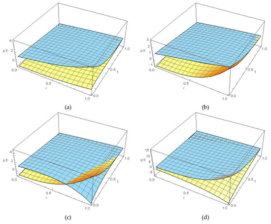
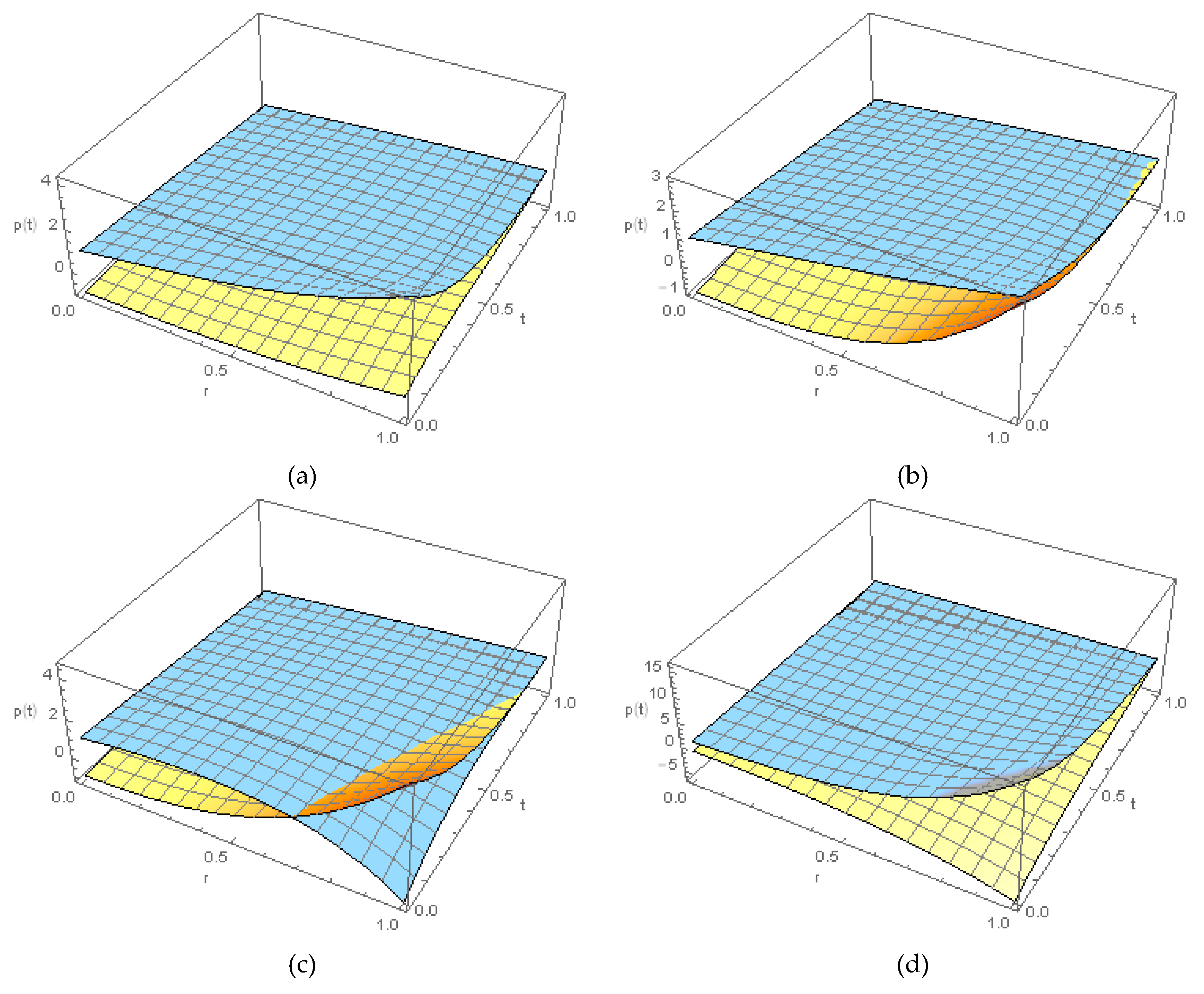
According to the RPSM algorithm, the solution details for each case of Equations (15) and (16) can be found in Appendix A. However, to show the effectiveness of the proposed algorithm, numerical outcomes of lower and upper bounds of the fuzzy solutions of fuzzy Duffing oscillator (15) and (16) compared with the variational iteration method (VIM) [18], Maples numerical solution (MNS) [18], and the exact solutions are summarized in Table 1 at $t=0.1,$ $n=5$ and each at $r\in \left[0,1\right]$ with step size $0.25$. From this table, it can be observed that the lower and upper RPS-solutions for each $r$-level cut coincide with those results obtained by other methods. Table 2 shows the absolute and relative errors of the 5^th-RPS solutions for Equations (15) and (16) at $r=1$ and different values of $t$ in $\left[0,1\right]$, such that $t\in \left\{0.1,0.3,0.5,0.7,0.9\right\}$. While Table 3 and Table 4 display the fuzzy approximate solutions of (1,1)-system and (1,2)-system, respectively, at various values of $r\in \left[0,1\right]$, with step size $0.25$ and various values of $t$, such that $t\in \left\{0.2,0.4,0.6,0.8\right\}$. From these results, we conclude that the results are in good agreement with each other in our two cases and are closer to solutions at $r=1$, as $r$ values increase. In any case, to demonstrate the 5^th-order RPS solutions behavior of Equations (15) and (16), the coupled surface has been plotted in a 3-dim graph for all possible $(n,m)$-systems of Equations (15) and (16) for each $t\in \left[0,1\right]$ and $r\in \left[0,1\right],$ as shown in Figure 1, whereas blue and yellow correspond to upper and lower bounds of the fuzzy solutions, respectively.

Table 1. Numerical comparison of approximate solutions of Equation (15) at $t=0.1$.

Lower ${\mathit{p}}_{\mathbf{5}\mathbf{,}\mathbf{1}\mathit{r}}\mathbf{\left(}\mathit{t}\mathbf{\right)}$	$\mathit{r}$	RPSM	VIM [18]	Exact Solution	MNS [18]
	$0$	$-0.9946548333$	$-0.9946548745$	$-0.9946548739$	$-0.9946548688$
	$0.25$	$-0.7176218148$	$-0.7176219076$	$-0.7176219071$	$-0.7176219141$
	$0.5$	$-0.4435578646$	$-0.4435578806$	$-0.4435578799$	$-0.4435578164$
	$0.75$	$-0.1714170902$	$-0.1714170389$	$-0.1714170382$	$-0.1714169861$
	$1$	$0.09983341667$	$0.09983341601$	$0.09983341664$	$0.09983341519$
Upper ${\mathit{p}}_{\mathbf{5}\mathbf{,}\mathbf{2}\mathit{r}}\mathbf{\left(}\mathit{t}\mathbf{\right)}$	$\mathit{r}$	RPSM	VIM [18]	Exact Solution	MNS [18]
	$0$	$1.19652366667$	$1.19652475384$	$1.19652475400$	$1.19652479981$
	$0.25$	$0.91852284342$	$0.91852280319$	$0.91852280370$	$0.91852292721$
	$0.5$	$0.64377182292$	$0.64377156027$	$0.64377156090$	$0.64377160488$
	$0.75$	$0.37122049382$	$0.37122034006$	$0.37122034070$	$0.37122034586$
	$1$	$0.09983341667$	$0.09983341601$	$0.09983341664$	$0.09983341519$

Table 2. Absolute and relative errors for Equations (15) and (16) at $r=1$.

${\mathit{t}}_{\mathit{i}}$	Exact	RPS	Absolute Error	Relative Error
$0.1$	$0.0998334166$	$0.0998334167$	$1.98385\times {10}^{-11}$	$1.98716\times {10}^{-10}$
$0.3$	$0.2955202067$	$0.2955202500$	$4.33387\times {10}^{-8}$	$1.46652\times {10}^{-7}$
$0.5$	$0.4794255386$	$0.4794270833$	$1.54473\times {10}^{-6}$	$3.22204\times {10}^{-6}$
$0.7$	$0.6442176872$	$0.6442339166$	$1.62294\times {10}^{-5}$	$2.51925\times {10}^{-5}$
$0.9$	$0.7833269096$	$0.7834207500$	$9.38404\times {10}^{-5}$	$1.19797\times {10}^{-4}$

Table 3. The r-level RPS solutions for system (17) at $n=5$.

${\mathit{p}}_{\mathbf{5}\mathbf{,}\mathbf{1}\mathit{r}}\mathbf{\left(}\mathit{t}\mathbf{\right)}$	${\mathit{t}}_{\mathit{i}}$	$\mathit{r}\mathbf{=}\mathbf{0}$	$\mathit{r}\mathbf{=}\mathbf{0.25}$	$\mathit{r}\mathbf{=}\mathbf{0.5}$	$\mathit{r}\mathbf{=}\mathbf{0.75}$	$\mathit{r}\mathbf{=}\mathbf{1}$
	$0.2$	$-0.9771546$	$-0.6691458$	$-0.3736266$	$-0.0858586$	$0.1986693$
	$0.4$	$-0.8961493$	$-0.5171258$	$-0.1924533$	$0.1028372$	$0.3894187$
	$0.6$	$-0.7369840$	$-0.2862825$	$0.0351700$	$0.3022108$	$0.5646480$
	$0.8$	$-0.4799786$	$0.0165733$	$0.2790933$	$0.4837893$	$0.7173973$
${\mathit{p}}_{\mathbf{5}\mathbf{,}\mathbf{2}\mathit{r}}(\mathit{t})$	${\mathit{t}}_{\mathit{i}}$	$\mathit{r}\mathbf{=}\mathbf{0}$	$\mathit{r}\mathbf{=}\mathbf{0.25}$	$\mathit{r}\mathbf{=}\mathbf{0.5}$	$\mathit{r}\mathbf{=}\mathbf{0.75}$	$\mathit{r}\mathbf{=}\mathbf{1}$
	$0.2$	$-0.9771547$	$1.0753739$	$0.7743423$	$0.4836909$	$0.1986693$
	$0.4$	$-0.8961493$	$1.3645042$	$0.9931466$	$0.6754232$	$0.3894187$
	$0.6$	$-0.7369840$	$1.6325016$	$1.1433200$	$0.8082544$	$0.5646480$
	$0.8$	$-0.4799787$	$1.8847333$	$1.2022933$	$0.8625413$	$0.7173973$

Table 4. The r-level RPS solutions for system (18) at $n=5$.

${\mathit{p}}_{\mathbf{5}\mathbf{,}\mathbf{1}\mathit{r}}(\mathit{t})$	${\mathit{t}}_{\mathit{i}}$	$\mathit{r}\mathbf{=}\mathbf{0}$	$\mathit{r}\mathbf{=}\mathbf{0.25}$	$\mathit{r}\mathbf{=}\mathbf{0.5}$	$\mathit{r}\mathbf{=}\mathbf{0.75}$	$\mathit{r}\mathbf{=}\mathbf{1}$
	$0.2$	$-0.9662910$	$-0.6665720$	$-0.3743330$	$-0.0868917$	$0.1986693$
	$0.4$	$-0.7853010$	$-0.4816390$	$-0.1870450$	$0.1009540$	$0.3894187$
	$0.6$	$-0.2786320$	$-0.1152050$	$0.0931120$	$0.3195730$	$0.5646480$
	$0.8$	$0.8143570$	$0.5461570$	$0.5161490$	$0.5863333$	$0.7173973$
${\mathit{p}}_{\mathbf{5}\mathbf{,}\mathbf{2}\mathit{r}}(\mathit{t})$	${\mathit{t}}_{\mathit{i}}$	$\mathit{r}\mathbf{=}\mathbf{0}$	$\mathit{r}\mathbf{=}\mathbf{0.25}$	$\mathit{r}\mathbf{=}\mathbf{0.5}$	$\mathit{r}\mathbf{=}\mathbf{0.75}$	$\mathit{r}\mathbf{=}\mathbf{1}$
	$0.2$	$-0.9662910$	$1.0746048$	$0.7763790$	$0.4854010$	$0.1986693$
	$0.4$	$-0.7853010$	$1.3578921$	$1.0077386$	$0.6881310$	$0.3894187$
	$0.6$	$-0.2786320$	$1.6076042$	$1.1866280$	$0.8456930$	$0.5646480$
	$0.8$	$0.8143570$	$1.8171493$	$1.2852373$	$0.9331970$	$0.7173973$

Figure 1. Surface plots of Equations (15) and (16) at $t\in \left[0,1\right]$ and $r\in \left[0,1\right]$: (a) (1,1)-system; (b) (1,2)-system; (c) (2,1)-system; (d) (2,2)-system, where blue and yellow represent the lower and upper boundaries, respectively, of 5th-RPS fuzzy solutions.

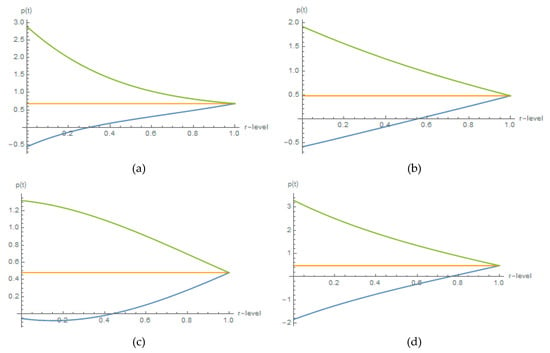
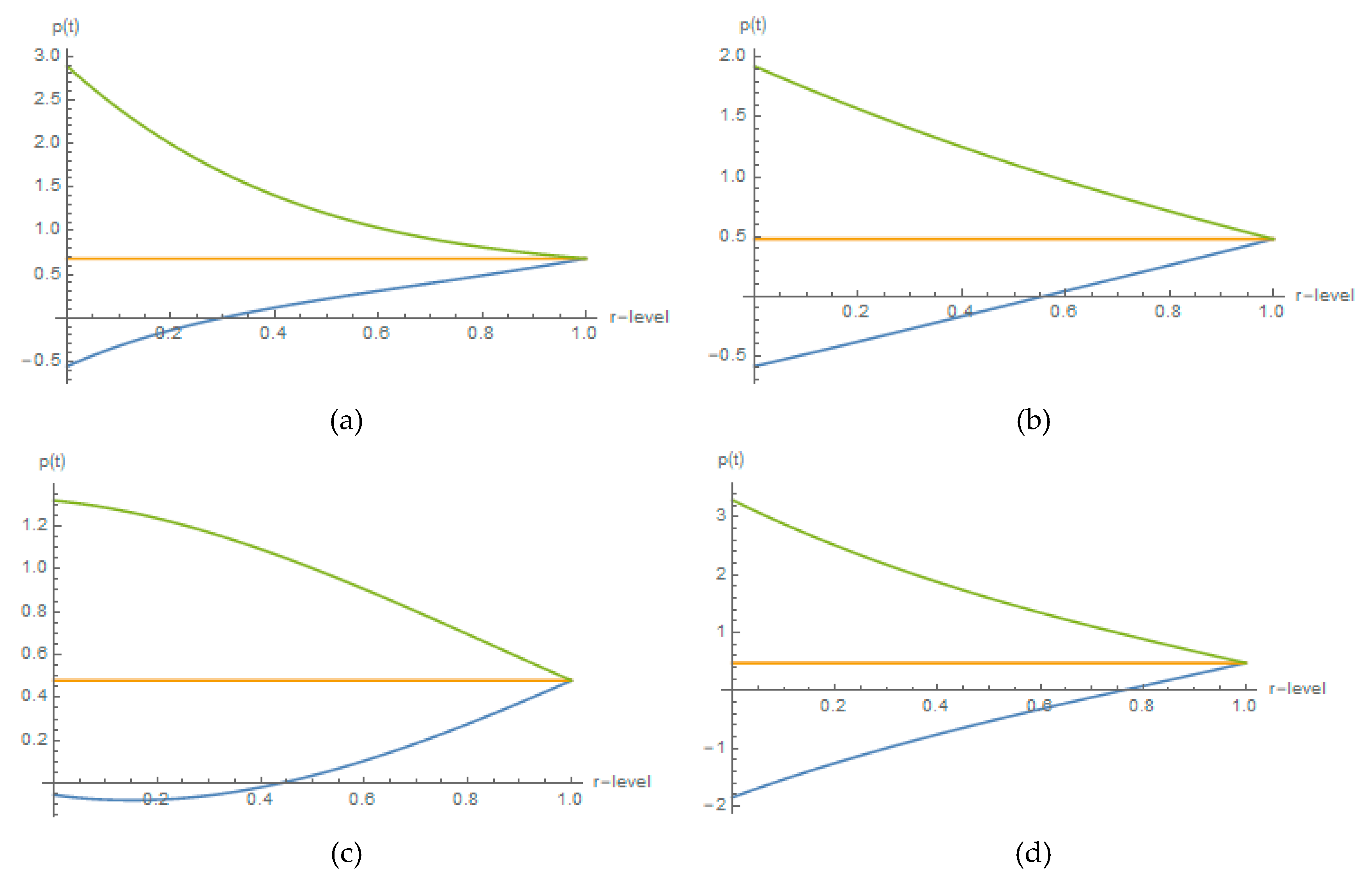
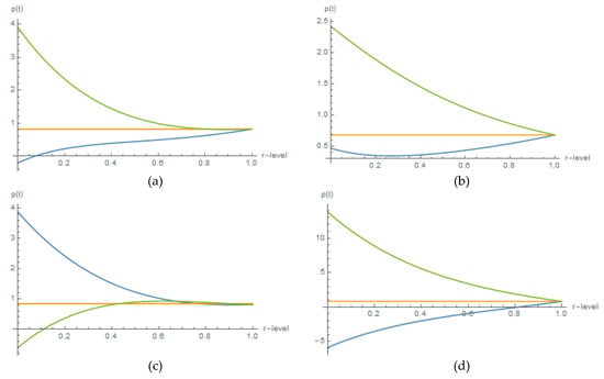
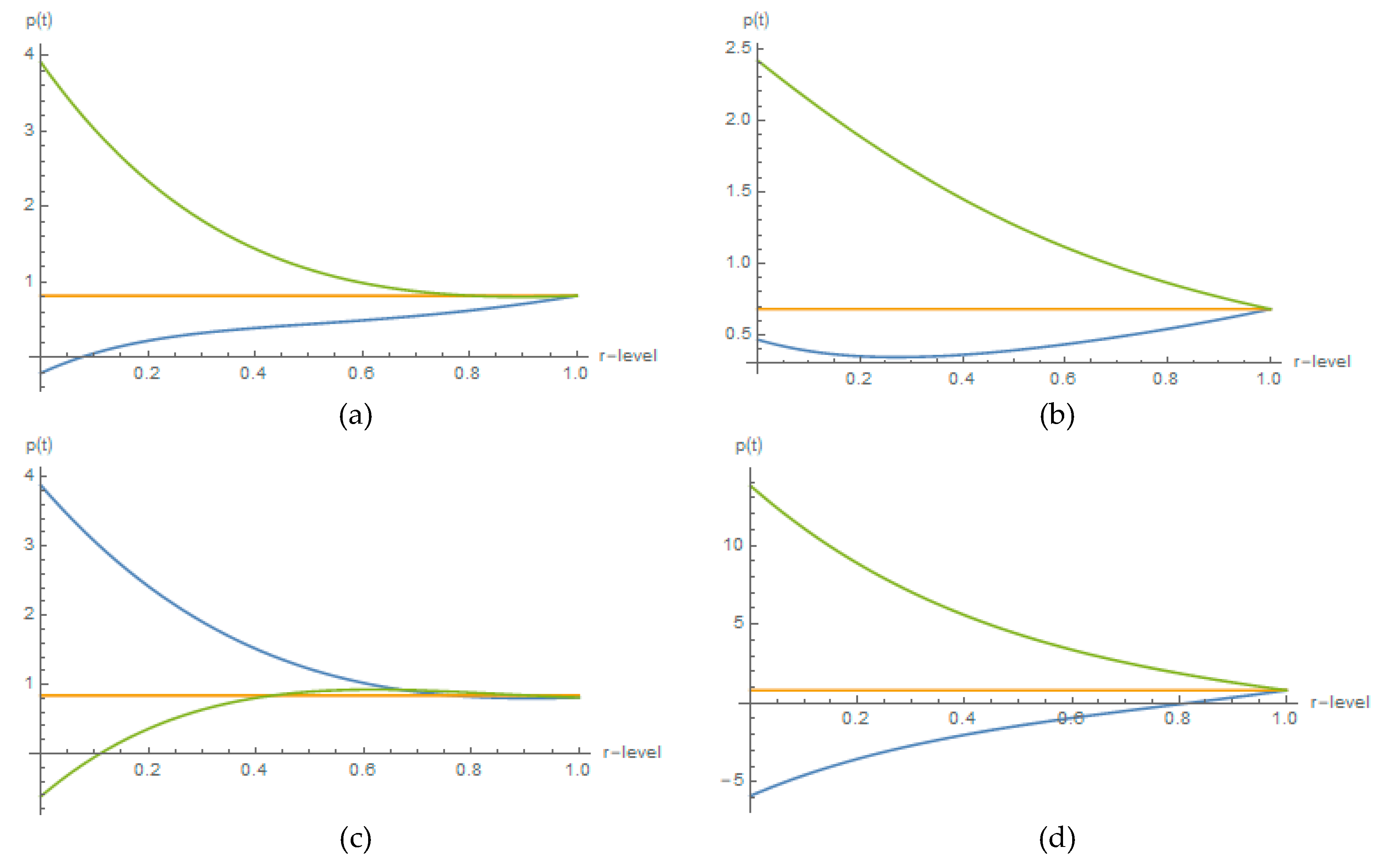
Figure 2 and Figure 3 depict the lower and upper bounds of triangular fuzzy solutions at $n=5$, with different values of $t$ such that $t=0.5$, as shown in Figure 2 and $t=0.95$, as shown in Figure 3, in which green and blue represent the lower and upper bounds of triangular fuzzy solutions, respectively, while the orange midline represents the solution at $r=1$.

Figure 2. Graphs of triangular fuzzy solutions of Equations (15) and (16) for each $r$ in $\left[0,1\right]$, n = 5 and t = 0.5: (a) (1,1)-solutions; (b) (1,2)-solutions; (c) (2,1)-solutions; (d) (2,2)-solutions, where green, blue and orange represent p_1r(0.5), p_2r(0.5) and p(0.5) at r = 1, respectively.

Figure 3. Graphs of triangular fuzzy solutions of Equations (15) and (16) for each $r$ in [0, 1], n = 5 and t = 0.95: (a) (1,1)-solutions; (b) (1,2)-solutions; (c) (2,1)-solutions; (d) (2,2)-solutions, where green, blue and orange represent p_1r(0.95), p_2r(0.95) and p(0.95) at r = 1, respectively.

Application 2.

Consider the following nonlinear fuzzy Duffing’s oscillator [18]:

$$p^{″}(t)+p^{\prime }(t)+p^3(t)=0,t\ge 0,$$

(21)

along with the following fuzzy initial conditions

$${\left[p(0)\right]}^r=\left[0.9+0.1r,1.1-0.1r\right]\mathrm{and}{\left[p^{\prime }(0)\right]}^r=\left[0.9+0.1r,1.1-0.1r\right],$$

(22)

where$r\in \left[0,1\right].$

This model can be regarded as an example of a nonlinear, nonharmonic, damped driven oscillator system with a nonlinear elasticity, whose restoring force can be written as $F=-p(t)-p^3(t)$. However, this model does not have an exact analytical solution.

According to Algorithm 1, the fuzzy Duffing oscillator (21) and (22) can be converted into four possible, crisp systems of ODEs, according to their parametric forms, as follows:

Case 1: If $p(t)$ is (1,1)- solution, then the corresponding (1,1)-system is

$$\{\begin{array}{c}{p}_{1r}^{″}(t)+p_{1r}^{\prime }(t)+p_{1r}^3(t)=0,\\ p_{2r}^{″}(t)+p_{2r}^{\prime }(t)+p_{2r}^3(t)=0,\\ p_{1r}(0)=0.9+0.1r, p_{1r}^{\prime }(0)=0.9+0.1r,\\ p_{2r}(0)=1.1-0.1r, p_{2r}^{\prime }(0)=1.1-0.1r.\end{array}$$

(23)

Case 2: If $p(t)$ is (1,2)-solution, then the corresponding (1,2)-system is

$$\{\begin{array}{c}{p}_{2r}^{″}(t)+p_{1r}^{\prime }(t)+p_{1r}^3(t)=0,\\ p_{1r}^{″}(t)+p_{2r}^{\prime }(t)+p_{2r}^3(t)=0,\\ p_{1r}(0)=0.9+0.1r, p_{1r}^{\prime }(0)=0.9+0.1r,\\ p_{2r}(0)=1.1-0.1r, p_{2r}^{\prime }(0)=1.1-0.1r.\end{array}$$

(24)

Case 3: If $p(t)$ is (2,1)-solution, then the correspondence (2,1)-system is

$$\{\begin{array}{c}{p}_{2r}^{″}(t)+p_{2r}^{\prime }(t)+p_{1r}^3(t)=0,\\ p_{1r}^{″}(t)+p_{1r}^{\prime }(t)+p_{2r}^3(t)=0,\\ p_{1r}(0)=0.9+0.1r, p_{1r}^{\prime }(0)=0.9+0.1r ,\\ p_{2r}(0)=1.1-0.1r, p_{2r}^{\prime }(0)=1.1-0.1r.\end{array}$$

(25)

Case 4: If $p(t)$ is (2,2)-solution, then the correspondence (2,2)-system is

$$\{\begin{array}{c}{p}_{1r}^{″}(t)+p_{2r}^{\prime }(t)+p_{1r}^3(t)=0,\\ p_{2r}^{″}(t)+p_{1r}^{\prime }(t)+p_{2r}^3(t)=0,\\ p_{1r}(0)=0.9+0.1r, p_{1r}^{\prime }(0)=0.9+0.1r,\\ p_{2r}(0)=1.1-0.1r, p_{2r}^{\prime }(0)=1.1-0.1r.\end{array}$$

(26)

According to the RPSM algorithm, the solution details for each case of FVIPs (21) and (22) can be found in Appendix A. However, since this model does not have an exact solution, so to illustrate the efficiency and accuracy of RPS algorithm, the following residual error is defined

$$E(t;r)=\left|p_n^{″}(t;r)+p_n(t;r)+{(p_n(t;r))}^3\right|.$$

(27)

To demonstrate the effectiveness of the RPS method for solving Equations (21) and (22), the lower and upper bounds of 10^th-RPS approximate solutions of (1,1)-system, with their residual errors, are computed and listed in Table 5 for $t=0.1$ and $r\in \left[0,1\right]$ with step size $0.25$, which can illustrate the efficiency of the proposed method.

Table 5. Lower and upper bound solutions of 10^th-RPS approximation at $t=0.1$.

$\mathit{r}$	Lower Bound		Upper Bound
	${\mathit{p}}_{1\mathit{r}}\mathbf{\left(}\mathit{t}\mathbf{\right)}$	${\mathit{E}}_1\mathbf{\left(}\mathit{t}\mathbf{;}\mathit{r}\mathbf{\right)}$	${\mathit{p}}_{\mathbf{2}\mathit{r}}\mathbf{\left(}\mathit{t}\mathbf{\right)}$	${\mathit{E}}_{\mathbf{2}}\mathbf{\left(}\mathit{t}\mathbf{;}\mathit{r}\mathbf{\right)}$
$0$	$0.9813481271$	$6.32899\times {10}^{-10}$	$1.1970156393$	$7.95815\times {10}^{-10}$
$0.25$	$1.0083764337$	$7.17582\times {10}^{-10}$	$1.1701305851$	$9.18593\times {10}^{-10}$
0.5	$1.0353857847$	$8.00644\times {10}^{-10}$	$1.1432235606$	$9.68646\times {10}^{-10}$
0.75	$1.0623756761$	$8.76832\times {10}^{-10}$	$1.1162950665$	$9.67723\times {10}^{-10}$
1	$1.0893456043$	$9.38968\times {10}^{-10}$	$1.0893456043$	$9.38968\times {10}^{-10}$

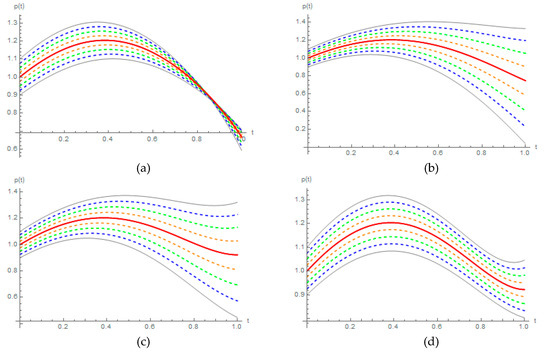
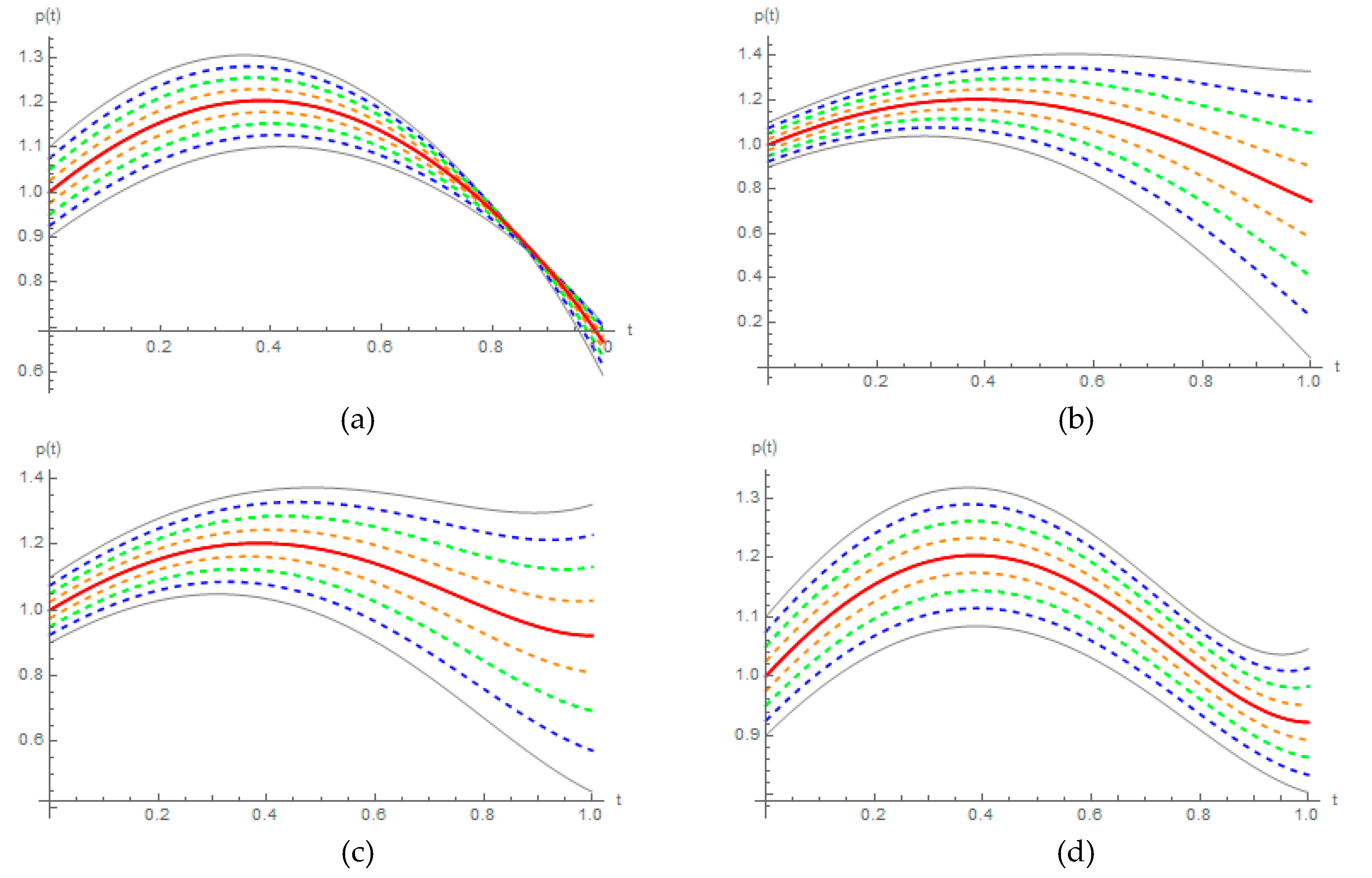
Symmetry is generally found in many mathematical works involving the fuzzy systems and fuzzy logic, if not most of them. When a fuzzy system is modeled, it naturally tends to choose symmetric features, the fuzzy membership functions that often designed regularly and symmetrically over the universal convex domain. Unfortunately, this does not always happen if features are automatically generated. So, researchers usually continue to study symmetrical fuzzy systems, using a deliberate lack of symmetry. In any case, Figure 4 shows the solution behavior of $r$-level 6^th-RPS approximate solutions for each possible $(n,m)$-systems of Equations (21) and (22) at $t\in \left[0,1\right]$ and $r\in \left\{0,0.25,0.5,0.75,1\right\}$, which guides us to a deep understanding of the pattern behavior of the fuzzy Duffing oscillator, in which gray, blue, green, orange and red refer to the $r$-level solutions at $r=0$, $r=0.25$, $r=0.5$, $r=0.75$ and $r=1$, respectively. The graphs of the $r$-level solutions of the fuzzy Duffing equation are implemented and presented in patterns similar to the interference patterns. The solutions to each case of the fuzzy Duffing equations are compatible with each other in some very simple way and slip into each other in the same direction without any intersections, where the behavior of these solution curves is harmonic in a smooth way around central symmetry at $r=1$ (the red line in the middle, Figure 4).

Figure 4. Solution behavior for each case of Equations (21) and (22) based on r-level solutions at $t\in \left[0,1\right]$ and n = 6: (a) (1,1)-system; (b) (1,2)-system; (c) (2,1)-system; (d) (2,2)-system, where gray, blue, green, orange and red refer to the 6th-RPS solutions at r = 0, r = 0.25, r = 0.5, r = 0.75 and r = 1, respectively.

6. Conclusions

In this article, attractive RPS strategy has been extended and implemented to explore analytic-fuzzy approximate solution of damped driven nonlinear fuzzy Duffing oscillator occurring in nonharmonic oscillating phenomena. This method was used directly, by selecting appropriate fuzzy initial guesses to obtain the approximation solution in the series formula with precisely computed constructs, without the need for unphysical restrictive assumptions, linearization, or perturbation. Graphical and numerical results have illustrated the pattern behavior at different values of $t$ and $r$-level. The results indicated that the approximate solutions are coinciding with each other for the selected nods and parameters. Based on the graphical results, it can be concluded that the opposite boundaries of fuzzy solutions form a somewhat symmetric triangular around the central symmetry at $r=1$. Meanwhile, the r-level of the symmetrical fuzzy-valued solutions are smooth in the same direction without any intersections. From our results, we can also conclude that the proposed method is a systematic and suitable scheme to address many initial value problems under uncertainty and solve them with great potential in scientific and physical applications.

References

- Guo, M.; Xue, X.; Li, R. Impulsive functional differential inclusions and fuzzy population models. Fuzzy Sets Syst. 2003, 138, 601–615. [Google Scholar] [CrossRef] [Scilit]
- Dubois, D.; Prade, H. Towards fuzzy differential calculus. Fuzzy Sets Syst. 1982, 8, 1–7. [Google Scholar] [CrossRef] [Scilit]
- Seikkala, S. On the fuzzy initial value problem. Fuzzy Sets Syst. 1987, 24, 319–330. [Google Scholar] [CrossRef] [Scilit]
- Al-Smadi, M. Reliable Numerical Algorithm for Handling Fuzzy Integral Equations of Second Kind in Hilbert Spaces. Filomat 2019, 33, 583–597. [Google Scholar] [CrossRef] [Scilit]
- Bede, B.; Gal, S.G. Almost periodic fuzzy-number-value functions. Fuzzy Sets Syst. 2004, 147, 385–403. [Google Scholar] [CrossRef] [Scilit]
- Wang, Y.; An, J.-Y. Amplitude–frequency relationship to a fractional Duffing oscillator arising in microphysics and tsunami motion. J. Low Freq. Noise, Vibr. Act. Cont. 2019, 38, 1008–1012. [Google Scholar]
- Nijmeijer, H.; Berghuis, H. On Lyapunov Control of the Duffing Equation. IEEE Trans. Circuits Syst. I 1995, 42, 473–477. [Google Scholar] [CrossRef]
- Yusufoglu, E. Numerical Solution of Duffing Equation by the Laplace Decomposition Algorithm. Appl. Math. Compu. 2006, 177, 572–580. [Google Scholar]
- Feng, Z. Duffing’s equation and its applications to the Hirota equation. Phys. Lett. A 2003, 317, 115–119. [Google Scholar] [CrossRef] [Scilit]
- Feng, Z. Monotonous property of non-oscillations of the damped Duffing’s equation. Chaos Solitons Fractals 2006, 28, 463–471. [Google Scholar] [CrossRef] [Scilit]
- Chen, Y.Z. Solution of the Duffing equation by using target function method. J. Soun. Vibr. 2002, 256, 573–578. [Google Scholar] [CrossRef] [Scilit]
- Attia, R.A.M.; Lu, D.; Khater, M.M.A. Chaos and Relativistic Energy-Momentum of the Nonlinear Time Fractional Duffing Equation. Math. Comput. Appl. 2019, 24, 10. [Google Scholar] [CrossRef] [Scilit]
- Abu Arqub, O.; Al-Smadi, M.; Momani, S.; Hayat, T. Application of reproducing kernel algorithm for solving second-order, two-point fuzzy boundary value problems. Soft Comput. 2017, 21, 7191–7206. [Google Scholar] [CrossRef] [Scilit]
- Alaroud, M.; Al-Smadi, M.; Ahmad, R.R.; Salma Din, U.K. An Analytical Numerical Method for Solving Fuzzy Fractional Volterra Integro-Differential Equations. Symmetry 2019, 11, 205. [Google Scholar] [CrossRef] [Scilit]
- Abu Arqub, O.; Al-Smadi, M.; Momani, S.; Hayat, T. Numerical solutions of fuzzy differential equations using reproducing kernel Hilbert space method. Soft Comput. 2016, 20, 3283–3302. [Google Scholar] [CrossRef] [Scilit]
- Gumah, G.N.; Naser, M.F.M.; Al-Smadi, M.; Al-Omari, S.K. Application of reproducing kernel Hilbert space method for solving second-order fuzzy Volterra integro-differential equations. Adv. Diff. Equ. 2018, 2018, 475. [Google Scholar] [CrossRef] [Scilit]
- Ahmad, N.I.; Mamat, M.; Kavikumar, J.; Hamzad, N.A. Solving Fuzzy Duffing’s Equation by the Laplace Transform Decomposition. Appl. Math. Sci. 2012, 6, 2935–2944. [Google Scholar]
- Jameel, A.F. The Variational Iteration Method for Solving Fuzzy Duffing’s Equation. J. Interp. Approx. Sci. Comput. 2014, 2014, 1–14. [Google Scholar] [CrossRef] [Scilit]
- Abu Arqub, O. Series solution of fuzzy differential equations under strongly generalized differentiability. J. Adv. Res. Appl. Math. 2013, 5, 31–52. [Google Scholar] [CrossRef] [Scilit]
- Freihet, A.; Hasan, S.; Al-Smadi, M.; Gaith, M.; Momani, S. Construction of fractional power series solutions to fractional stiff system using residual functions algorithm. Adv. Differ. Equ. 2019, 2019, 95. [Google Scholar] [CrossRef] [Scilit]
- Freihet, A.; Hasan, S.; Alaroud, M.; Al-Smadi, M.; Ahmad, R.R.; Din, S.K.U. Toward computational algorithm for time-fractional Fokker-Planck models. Adv. Mech. Eng. 2019, 11, 1–11. [Google Scholar] [CrossRef] [Scilit]
- Shammari, M.A.; Al-Smadi, M.; Abu Arqub, O.; Hashim, I.; Alias, M.A. Adaptation of residual power series method to solve Fredholm fuzzy integro-differential equations. AIP Conf. Proc. 2019, 2111, 020002. [Google Scholar]
- Momani, S.; Abu Arqub, O.; Freihat, A.; Al-Smadi, M. Analytical approximations for Fokker-Planck equations of fractional order in multistep schemes. Appl. Comput. Math. 2016, 15, 319–330. [Google Scholar]
- Hasan, S.; Al-Smadi, M.; Freihet, A.; Momani, S. Two computational approaches for solving a fractional obstacle system in Hilbert space. Adv. Differ. Equ. 2019, 2019, 55. [Google Scholar] [CrossRef] [Scilit]
- Al-Smadi, M. Simplified iterative reproducing kernel method for handling time-fractional BVPs with error estimation. Ain Shams Eng. J. 2018, 9, 2517–2525. [Google Scholar] [CrossRef] [Scilit]
- Shqair, M.; Al-Smadi, M.; Momani, S.; El-Zahar, E. Adaptation of conformable residual power series scheme in solving nonlinear fractional quantum mechanics problems. Appl. Sci. 2020, 10, 890. [Google Scholar] [CrossRef] [Scilit]
- Alshammari, S.; Al-Smadi, M.; Al Shammari, M.; Hashim, I.; Alias, M.A. Advanced analytical treatment of fractional logistic equations based on residual error functions. Int. J. Differ. Equ. 2019, 2019, 7609879. [Google Scholar] [CrossRef] [Scilit]
- Saadeh, R.; Alaroud, M.; Al-Smadi, M.; Ahmad, R.R.; Salma Din, U.K. Application of fractional residual power series algorithm to solve Newell–Whitehead–Segel equation of fractional order. Symmetry 2019, 11, 1431. [Google Scholar] [CrossRef] [Scilit]
- Alshammari, S.; Al-Smadi, M.; Hashim, I.; Alias, M.A. Residual Power Series Technique for Simulating Fractional Bagley–Torvik Problems Emerging in Applied Physics. Appl. Sci. 2019, 9, 5029. [Google Scholar] [CrossRef] [Scilit]
- Alshammari, S.; Al-Smadi, M.; Hashim, I.; Alias, M.A. Applications of fractional power series approach in solving fractional Volterra integro-differential equations. AIP Conf. Proc. 2019, 2111, 020003. [Google Scholar]
- Al-Smadi, M.; Freihat, A.; Abu Arqub, O.; Shawagfeh, N. A novel multistep generalized differential transform method for solving fractional-order Lü chaotic and hyperchaotic systems. J. Comput. Anal. Appl. 2015, 19, 713–724. [Google Scholar]
- Al-Smadi, M.; Abu Arqub, O. Computational algorithm for solving fredholm time-fractional partial integrodifferential equations of dirichlet functions type with error estimates. Appl. Math. Comput. 2019, 342, 280–294. [Google Scholar] [CrossRef] [Scilit]
- Hasan, S.; El-Ajou, A.; Hadid, S.; Al-Smadi, M.; Momani, S. Atangana-Baleanu fractional framework of reproducing kernel technique in solving fractional population dynamics system. Chaos Solitons Fractals 2020, 133, 109624. [Google Scholar] [CrossRef] [Scilit]
- Abu Arqub, O.; Al-Smadi, M. Fuzzy conformable fractional differential equations: Novel extended approach and new numerical solutions. Soft Comput. 2020. [Google Scholar] [CrossRef] [Scilit]
- Goetschel, J.R.; Voxman, W. Elementary fuzzy calculus. Fuzzy Sets Syst. 1986, 18, 31–43. [Google Scholar] [CrossRef] [Scilit]
- Puri, M.L.; Ralescu, D.A. Differentials of fuzzy functions. J. Math. Anal. Appl. 1983, 91, 552–558. [Google Scholar] [CrossRef] [Scilit]
- Bede, B.; Gal, S.G. Generalizations of the differentiability of fuzzy-number-valued functions with applications to fuzzy differential equations. Fuzzy Sets Syst. 2005, 151, 581–599. [Google Scholar] [CrossRef] [Scilit]
- Chalco-Cano, Y.; Roman-Flores, H. On new solutions of fuzzy differential equations. Chaos Solitons Fractals 2008, 38, 112–119. [Google Scholar] [CrossRef] [Scilit]
- Khastan, A.; Bahrami, F.; Ivaz, K. New Results on Multiple Solutions for nth-Order Fuzzy Differential Equations under Generalized Differentiability. Bound. Value Probl. 2009, 2009, 395714. [Google Scholar] [CrossRef] [Scilit]
© 2020 by the authors. Licensee MDPI, Basel, Switzerland. This article is an open access article distributed under the terms and conditions of the Creative Commons Attribution (CC BY) license (http://creativecommons.org/licenses/by/4.0/).