Using Data Envelopment Analysis and Multi-Criteria Decision-Making Methods to Evaluate Teacher Performance in Higher Education

Abstract

This paper proposes an approach that combines data envelopment analysis (DEA) with the analytic hierarchy process (AHP) and conjoint analysis, as multi-criteria decision-making methods to evaluate teachers’ performance in higher education. This process of evaluation is complex as it involves consideration of both objective and subjective efficiency assessments. The efficiency evaluation in the presence of multiple different criteria is done by DEA and results heavily depend on their selection, values, and the weights assigned to them. Objective efficiency evaluation is data-driven, while the subjective efficiency relies on values of subjective criteria usually captured throughout the survey. The conjoint analysis helps with the selection and determining the relative importance of such criteria, based on stakeholder preferences, obtained as an evaluation of experimentally designed hypothetical profiles. An efficient experimental design can be either symmetric or asymmetric depending on the structure of criteria covered by the study. Obtained importance might be a guideline for selecting adequate input and output criteria in the DEA model when assessing teachers’ subjective efficiency. Another reason to use conjoint preferences is to set a basis for weight restrictions in DEA and consequently to increase its discrimination power. Finally, the overall teacher’s efficiency is an AHP aggregation of subjective and objective teaching and research efficiency scores. Given the growing competition in the field of education, a higher level of responsibility and commitment is expected, and it is therefore helpful to identify weaknesses so that they can be addressed. Therefore, the evaluation of teachers’ efficiency at the University of Belgrade, Faculty of Organizational Sciences illustrates the usage of the proposed approach. As results, relatively efficient and inefficient teachers were identified, the reasons and aspects of their inefficiency were discovered, and rankings were made.

1. Introduction

The sector of higher education and development, faced with competitive pressure, carries a great responsibility to increase the efficiency of its activities continuously. Obviously, higher education productivity has a multidimensional character as it relates to knowledge production and dissemination through both teaching and scientific research. Therefore, the evaluation of teachers’ performance is a more challenging issue because it involves multiple criteria as objectives.

Following the standards for assessing the quality of teachers’ work, one of the measuring instruments is student satisfaction [1]. An important factor affecting the satisfaction of the students, as the users of higher education services, with the education process, is the professional and practical knowledge of the teachers and their academic assessment [2,3,4]. Therefore, at many higher education institutions, students are offered some kind of evaluation in which they rate the teaching process and the competencies of the teachers for each course [5,6,7].

Data envelopment analysis (DEA) is an approach to measure the relative efficiency of decision-making units (DMUs) that are characterized by multiple incommensurate inputs and outputs. Its results rely heavily on the set of criteria used in the analysis. Therefore, one of the most important stages in the DEA is the selection of criteria, especially as the effort of evaluation increases significantly with the increase in the amount of data available. In a number of studies, researchers treat inputs and outputs simply as “givens” and then proceed to deal with the DEA methodology [8]. On the other hand, the analytic hierarchy process (AHP) and conjoint analysis are multi-criteria decision-making methods (MCDM) that can provide a priori information about the significance of inputs and outputs.

Although the theoretical foundations and methodological frameworks of conjoint analysis and AHP methods are different, they can be used independently and comparatively in similar or even the same studies [9,10,11,12,13,14,15]. Both methods can be used to measure respondents’ preferences as well as to determine the relative importance of attributes, but still the choice of the appropriate one depends on the particular problem and aspects of the research [16].

DEA models can be combined with AHP in numerous ways [17]. According to the literature, the AHP method is used in cases when the following are necessary: complete ranking in a two-stage process [18,19,20,21]; estimating missing data [22]; imposing weight restrictions [23,24,25,26,27]; reducing the number of input or output criteria [28,29,30], and converting qualitative data to quantitative [31,32,33,34,35,36,37,38,39,40,41]. The only paper published so far that has had the idea of combining the DEA method with conjoint analysis is by Salhieh and Al-Harris [42]. They suggested combining these methods for selecting new products on the market.

This paper presents a new approach for measuring the overall teachers’ efficiency as a weighted sum of subjective and objective efficiency scores. The approach integrates DEA with the AHP and conjoint analysis as multi-criteria decision-making methods. The AHP enables the creation of a hierarchical structure used to configure the problem of the overall efficiency evolution. Furthermore, the weights of all efficiency measures at the highest level of the hierarchy are obtained using AHP. The procedure of assessing subjective efficiency consists of the conjoint analysis and DEA. The conjoint analysis is finding out the relative importance of each criterion, based on stakeholder preferences, afterwards used as guidelines for the DEA criteria selection. Another reason to use conjoint preferences is to set a basis for weight restrictions imposed in DEA models. The objective teaching and research efficiency scores are assessed by applying traditional DEA models. The proposed approach provides the determination of scores and ranking of relatively efficient and inefficient teachers as well as strong and weak aspects of their teaching and research work.

The paper is structured as follows: Section 2 describes the DEA basics and the implementation process, followed by a literature survey concerning criteria (input and output) selection. Conjoint analysis and the AHP method, including an approach for determining the importance of the criteria considered, are also presented in this section. A new methodological framework for combining conjoint analysis, AHP, and DEA are presented in Section 3. An illustration of the proposed methodology and real-world test results are given in Section 4. Section 5 provides the main conclusions and directions of future research.

2. Background

2.1. Data Envelopment Analysis

The creators of DEA, Charnes, Cooper, and Rhodes [43], introduced the basic DEA model (the so-called CCR DEA model) in 1978 as a new way to measure the efficiency of DMUs using multiple inputs and outputs. Since then, many variations of DEA models have been developed. Some of them are: the BCC DEA model proposed by Banker, Charnes, and Cooper [44], which assumes variable return to scale; the additive model [45], which is non-radial; the Banker and Morey [46] model that involves qualitative inputs and outputs; and the Golany and Roll [47] model, with restricted input and/or output weights to specific ranges of values. DEA empirically identifies the data-driven frontier of efficiency, which envelopes inefficient DMUs while efficient DMUs lie on the frontier. Let us assume that there are n DMUs, and the jth DMUs produce s outputs (y_ij, …, y_sj) by using m inputs (x_ij, …, x_mj). The basic output-oriented CCR DEA model is as follows:

$$\begin{array}{l}(\max )h_k={\displaystyle \sum _{r=1}^s{u}_r{y}_{rk}}\\ st\\ {\displaystyle \sum _{i=1}^m{v}_i{x}_{ik}}=1\\ {\displaystyle \sum _{r=1}^s{u}_r{y}_{rj}}-{\displaystyle \sum _{i=1}^m{v}_i{x}_{ij}}\le 0, j=1,\dots ,n\\ u_r\ge 0; r=1,2,\dots ,s,\\ v_i\ge 0; i=1,2,\dots ,m,\end{array}.$$

(1)

where $u_r,(r=1,2,\dots ,s),$ are weights assigned to the rth outputs, and $v_i, (i=1,2,\dots ,m),$ are weights assigned to the ith inputs, in order to assess maximal possible efficiency score. The score h_k shows relative efficiency of DMU_k, obtained as the maximum possible achievement in comparison with the other DMUs under the evaluation.

Emrouznejad and Witte [48] proposed a complete procedure for assessing DEA efficiency in large-scale projects, a so-called COOPER-framework, which can be further modified and adapted to the specific requirements of a particular study. The COOPER-framework consists of six phases: (1) Concepts and objectives, (2) On structuring data, (3) Operational models, (4) Performance comparison model, (5) Evaluation, and (6) Results and deployment. The first two phases involve defining the problem and understanding how the DMU works, while the last two phases involve producing a summary of the results and reporting.

In this paper, attention is paid to phases 1, 2, 3, and 4, since the objective definition in the model (1) obviously indicates that the efficiency of DMU_k is crucially related to the criteria selected. Jenkins and Anderson [49] claim that the more criteria there are, the less constrained weights are assigned to the criteria and the less discriminating the DEA scores are. The number of criteria may be substantial, and it may not be clear which one to choose. Moreover, the selection of different criteria can lead to different efficiency evaluation results. Of course, it is possible to consider all the criteria for evaluation. Still too many of them may lead to too many efficient units, and it may give rise to difficulties in distinguishing efficient units from inefficient ones. For this reason, the problem of selecting adequate criteria becomes an essential issue for improving the discrimination power of DEA.

There is no consensus on how to limit the number of criteria in the best way even though it is very advantageous. Banker et al. [44] suggest that the number of DMUs being evaluated should be at least three times the number of criteria. As noted by Golani and Roll [47], several studies emphasize the importance of the process of selecting data variables in addition to the DEA methodology itself. One approach is to select those criteria that are low-correlated. However, studies have shown that removing highly correlated criteria can still have a significant effect on DEA results [50]. Morita and Avkiran [51] used a three-level orthogonal layout experiment to select an appropriate combination of inputs and outputs based on external information. Edirisinghe and Zhang [52] proposed a two-step heuristic algorithm for criteria selection in DEA based on maximizing the correlation between DEA score and the external performance index.

Regardless of the method of criteria selection and the criteria, DEA does not allow discrimination between efficient DMUs because of their maximal efficiency. Several attempts to fully rank DMUs have been made, including modifying basic DEA models and connecting them to multi-criteria approaches [53]. The discrimination power of the DEA method can also be improved by promoting symmetric weight selection [54] by imposing penalizing differences in the values of each combination of two inputs or outputs. Other options are using cross-efficiency evolution [55] or imposing weight restrictions on models. A well-known assurance region DEA model (AR DEA) [56] imposes lower and upper boundaries on the weight ratio, as follows:

$$L_{1,2}\le \frac{v_2}{v_1}\le U_{1,2}.$$

(2)

An important consideration in the weight restrictions is setting realistic boundaries. In most cases, they are set on the basis of expert opinions and experience. Another direction can be DEA’s combination with other statistical methods to get data or evidence-driven boundaries [57]. In this paper, the results of the conjoint analysis are used to help determine the boundaries.

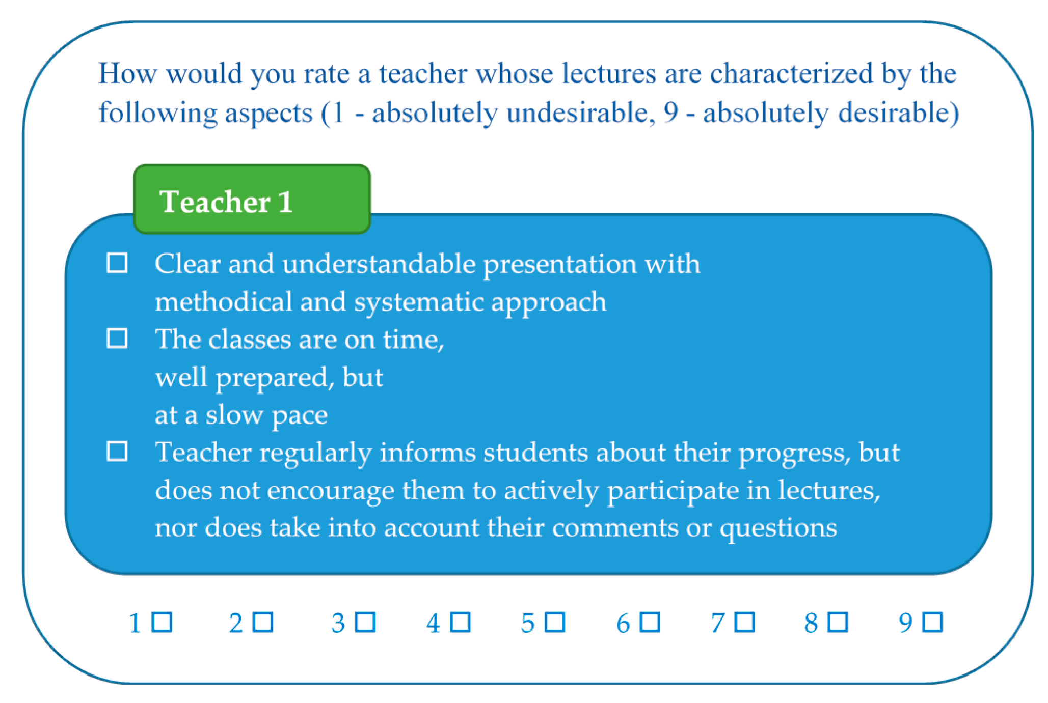
2.2. Conjoint Analysis

Conjoint analysis is a class of multivariate techniques used to understand individuals’ preferences better. A key goal of conjoint analysis is to identify which criteria most affects individuals’ choices or decisions, but also to find out how they make trade-offs between conflicting criteria.

The first step in conjoint analysis involves determining the set of key features (attributes, criteria) that describe an object (entity) and the levels of attributes that differentiate objects from one another. Sets of attribute levels that describe single alternatives are referred to as profiles. Depending on the number of attributes included in the study, a list of profiles that are presented to the respondent to evaluate can be either full factorial (all possible combinations of attribute levels) or fractional factorial (subset of all possible combinations) experimental design. Furthermore, fractional factorial designs could be either symmetric, if all attributes are assigned an equal number of levels, or asymmetric otherwise [58]. Both the ranking and rating approach can be used to evaluate profiles from the experimental design.

After collecting individuals’ responses, a model should be specified that relates those responses to the utilities of the attribute levels that are included in the certain profiles. The most commonly used model is the linear additive model of part-worth utilities. In the conjoint experiment with K attributes, each with L_k levels, model implies that the overall utility of the profile j (j = 1, …, J) for the respondent i (i = 1, …, I) can be expressed as follows [59]:

$$U_{ij}={\displaystyle \sum _{k=1}^K{\displaystyle \sum _{l=1}^{L_k}{\beta }_{ikl}{x}_{jkl}}}+{\epsilon }_{ij}$$

(3)

where x_jkl is a (0,1) variable that equals 1 if profile j contains lth level of attribute k, otherwise it equals 0. β_ikl is respondent i’s utility (part-worth) assigned to the level l of the attribute k; ε_ij is a stochastic error term.

Part-worths are estimated using the least square method and reflect the extent to which the selection of a particular profile is affected by these levels. The larger the variations of part-worths within an attribute, the more important the attribute is. Therefore, the relative importance of attribute k (k = 1, …, K) for respondent i (i = 1, …, I) can be expressed as the ratio of the utility range for a particular attribute and the sum of the utility ranges for all attributes [60]:

$$F{I}_{ik}=\frac{\underset{l}{\max }{\widehat{\beta }}_{ikl}-\underset{l}{\min }{\widehat{\beta }}_{ikl}}{{\displaystyle \sum _{k=1}^K\left(\underset{l}{\max }{\widehat{\beta }}_{ikl}-\underset{l}{\min }{\widehat{\beta }}_{ikl}\right)}}.$$

(4)

The resulting importance scores can be further used to calculate aggregated importance values. Estimated part-worth utilities can also be used as input parameters of the simulation models to predict how individuals will choose between competing alternatives, but also to examine how their choices change as the characteristics of the alternatives vary.

2.3. The Analytic Hierarchy Process (AHP)

The AHP is a MCDM method proposed by Saaty [61], which allows experts to prioritize decision criteria through a series of pairwise comparisons. There are three basic principles that AHP relies on: (1) the hierarchy principle, which involves constructing a hierarchical tree with criteria, sub-criteria, and alternative solutions; (2) the priority-establishing principle; and (3) the consistency principle [62].

In order to establish the various criteria weights, the AHP method uses their pairwise comparisons recorded a square matrix A. All elements on diagonal of matrix are 1. A decision maker compares elements in pairs at the same level of hierarchical structure using the Satie scale of relative importance. The same procedure is applied throughout the downward hierarchy until comparisons of all alternatives with respect to the parent sub-criteria at the (k-1) level are made at the last k-th level. The resulting elements at this stage are referred to as "local" weights. The mathematical model performs the aggregation of weights from different levels and gives the final result of the priorities of the alternatives in relation to the set goal.

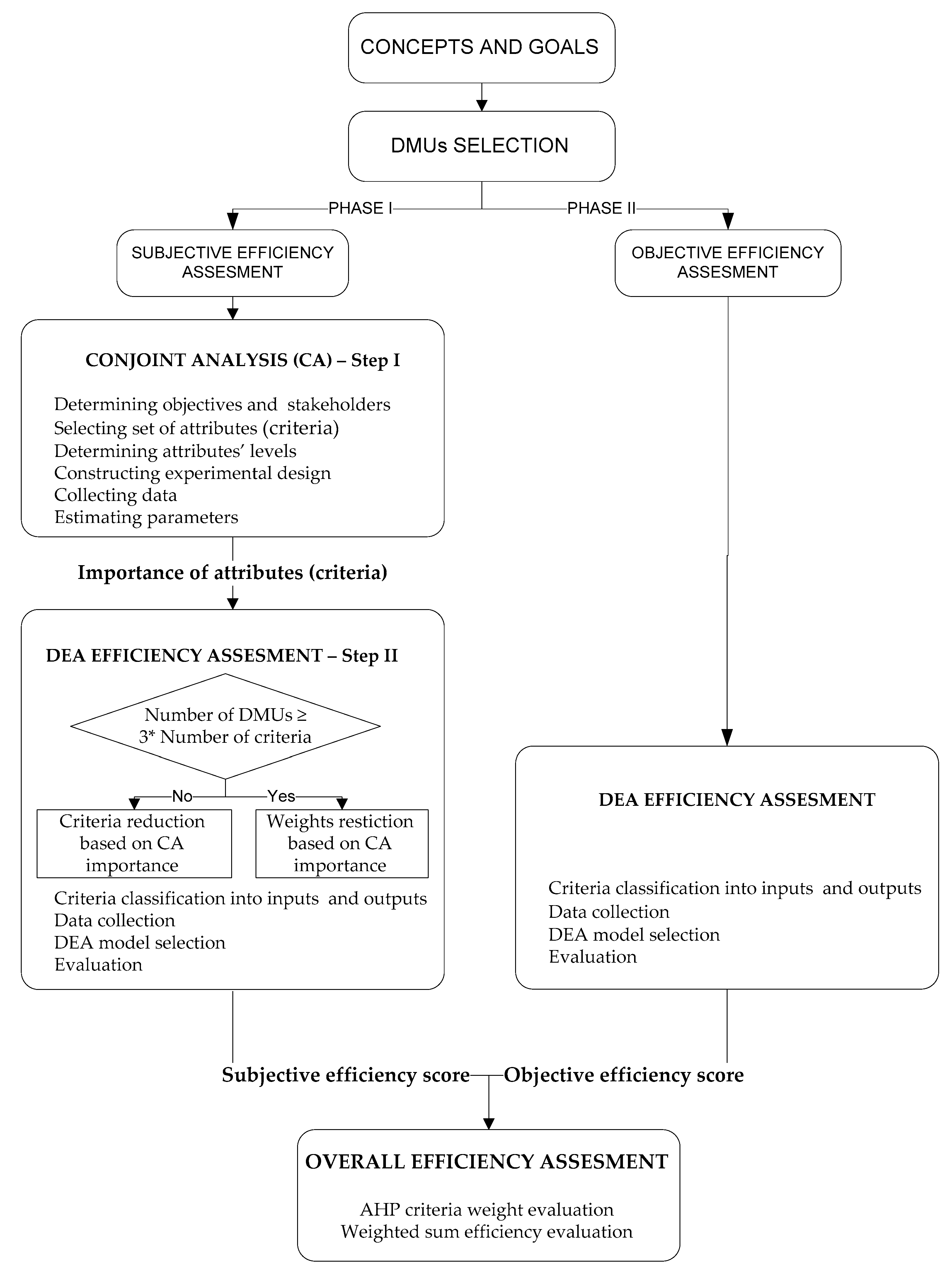
3. Methodological Framework

The following methodological framework is designed with the intention to make an aggregated efficiency assessment of the DMUs under consideration. The first step is to define the concepts and aims of the analysis, followed by the selection of the units under the evaluations. Afterwards, the efficiency scores are evaluated in an independent phase following the procedure proposed for subjective or objective efficiency assessment, shown in Figure 1.

Phase I of the methodological framework is an assessment of subjective efficiencies, which strongly depends on respondents’ opinions and preferences. Consequently, this efficiency is evaluated throughout two steps (Step 1—Conjoint preference analysis and Step 2—DEA efficiency assessment). Step 1 firstly defines the objectives of preference analysis and stakeholders as a starting point of this phase. Afterwards, the set of K key attributes (criteria) and their levels are selected based on the defined objectives. Secondly, experimental design is generated. It is the most sensitive stage of the conjoint analysis as the levels of the selected criteria should be combined to create different hypothetical profiles for the survey. The respondents (stakeholders) need to assign preference ratings towards each of the profiles from the generated experimental design. After making the most suitable experimental layout, conducting the survey, and collecting the data, the next stage assumes the estimating of the model’s parameters using statistical techniques and calculating the importance of the attributes FI_k, k = 1, …, K. The starting set of K criteria together with obtained importance values FI_k will be used as inputs for the next step.

Step II (Phase I), assumes the DEA efficiency evaluation. There are two possibilities for the analysis in the second step (DEA), depending on the total number (K) of criteria selected during Step I. In the first case, an analyst reduces the set of criteria to a suitable number (n ≤ 3 × K), by selecting them in descending order of stockholder’s preference FI_k, k = 1, …, K. In the second case, when the number of criteria is not too high, importance values FI_k are used for the weight restrictions to better discriminate between DMUs. This decision leads to the classification of selected criteria into the subsets of m inputs and n outputs depending on their nature, data collection, and DEA model selection. Finally, in this step, the chosen DEA model is solved to obtain the efficiency scores for each DMU in the observing set.

Phase II of the framework includes the objective DEA efficiency assessment. Unlike the subjective efficiency evaluation based on the stakeholders’ opinion, data-driven DEA efficiency is measured objectively, using the explicit data on the behavior of the system. Main steps are similar to the steps defined in the first phase: selecting input and outputs, collecting data, selecting the appropriate DEA model, and evaluation of the efficiency score.

Finally, the overall efficiency is calculated as a sum of products of all partial efficiency scores, subjective and objective, and their weights. The weights obtained using the AHP method, define the importance of all efficiency measures included in analysis.

The proposed procedure allows the combination of the subjective (Phase I) and objective efficiency measures (Phase II) obtained by DEA. The obtained measures are relative and data-driven. The subjective efficiency is made to be objective by using DEA for efficiency assessment and conjoint analysis for criteria importance evaluation. The main advantages and disadvantages of such a procedure come from DEA characteristics. On the one hand, there is no need for a priori weight imposing, data normalization, or production frontier determination. On the other hand, a small range of criteria values or a large number of criteria can lead to untrustworthy efficiency evaluation using the basic CCR DEA model. Step II (Phase I) tackles this issue. The conjoint preference analysis among stakeholders provides values of criteria importance that can be used for either criteria number reduction or criteria weight restrictions incorporated into DEA models. Both scenarios should lead to improved discrimination power based on DEA efficiency, which is the advantage of the proposed procedure. The procedure described above is illustrated in the next section using real data.

4. Empirical Study

Considering the importance of measuring and monitoring the performance of academic staff in both the teaching and research process, university teachers from the Faculty of Organizational Sciences were selected as DMUs in this study. Their overall efficiency should be measured from different aspects. Based on the proposed methodological framework the aggregated assessment of teacher’s efficiency was considered from two aspects: a subjective (assessment of teaching) and objective (teaching and research efficiency) aspect (see Figure 2). The AHP hierarchical structure is used for defining the problem of overall teachers’ efficiency, with overall teachers’ efficiency as a goal at the top level. The first and second levels of the hierarchy comprise subjective efficiency and two types of objective efficiencies, needed to be aggregated into overall efficiency. The second level of the hierarchy represents sub-criteria used as inputs and outputs in DEA efficiency assessment.

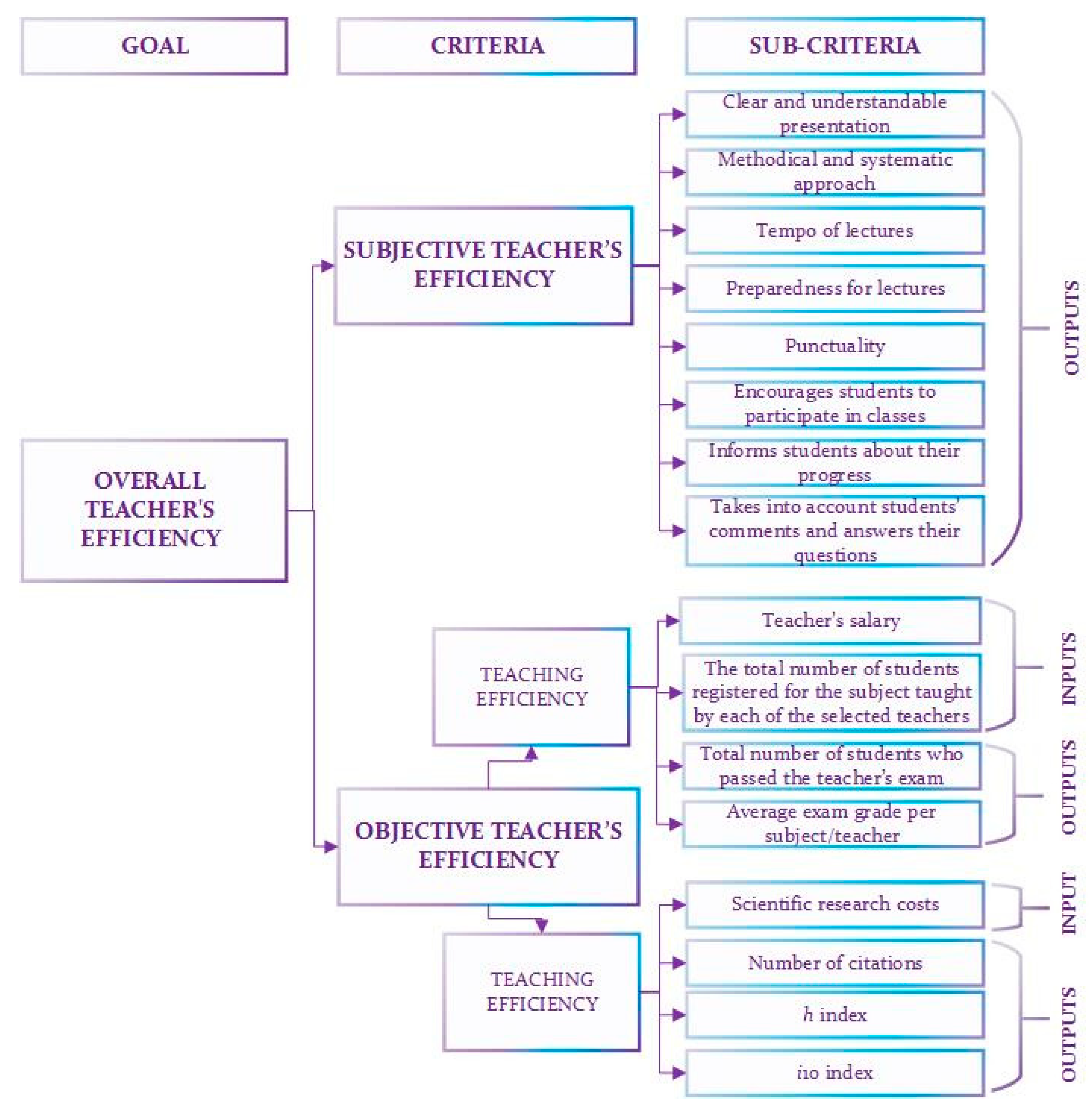
4.1. Subjective Assessment of Teacher’s Efficiency

The evaluation was carried out following the proposed methodological framework throughout Step I and Step II.

Step I. Students’ preferences toward eight criteria pre-set by university authorities were determined using conjoint analysis (see

Table 1. A set of criteria considered in the conjoint analysis survey, and the resulting utilities and importance values.

No	Criteria (Attributes)	Attribute Levels	Part-Worths (β)	Relative Importance Values (FI)
C1	Clear and understandable presentation of teaching content	Yes	0.865	22.98%
		No	−0.865
C2	Methodical and systematic approach to teaching	Yes	0.73	18.96%
		No	−0.73
C3	Tempo of lectures	Too slow	0.451	14.92%
		Optimal	−0.117
		Too fast	−0.334
C4	Preparedness for lectures	Good	0.266	7.96%
		Poor	−0.266
C5	Punctuality	On time	0.303	9.00%
		Late	−0.303
C6	Encouraging students to actively participate in classes	Yes	0.28	8.14%
		No	−0.28
C7	Informing students about their progress	Yes	0.324	9.08%
		No	−0.324
C8	Takes into account students’ comments and answers their questions	Yes	0.293	8.95%
		No	−0.293
	Constant		4.046
Correlations
Pearson’s R = 0.966 (sig. = 0.000)
Kendall’s tau = 0.933 (sig. = 0.000)
Kendall’s tau (for two holdouts) = 1.000

). An efficient experimental design of 16 profiles was constructed using the statistical package SPSS 16.0 (Orthoplan component). As all attributes did not have the same number of levels, the resulting design was asymmetric but orthogonal. In order to verify the consistency of students’ responses, two holdout profiles were added to the given design. A total of 106 third-year students from the Faculty of Organizational Sciences expressed their preferences for each of the 18 hypothetical teacher profiles in a nine-point Likert scale, with 1 referring to absolutely undesirable, and 9 to absolutely desirable profiles. An example of the hypothetical teacher profile evaluation task is given in Figure 3.

After removing the incomplete responses, 98 acceptable surveys remained, yielding a total of 1568 observations. The parameters were estimated for each student in the sample individually, and the sample as a whole. The averaged results and model fit statistics are shown in Table 1, indicating that the estimated parameters are highly significant.

The conjoint data presented in Table 1 indicate wide variations in the relative importance of the criteria considered. The most important criterion is the one concerning the clarity and comprehensibility of the teacher’s presentation (C1), followed by the criteria relating to the methodical and systematic approach to lectures (C2), and the tempo of lectures (C3). The three criteria listed cover more than 50% of the total importance, and these results were further used for the efficiency evaluation in step II.

Step II. DEA analyses were carried out in order to compare teachers, make a distinction between their performances, and find out advantages and disadvantages. The official database consists of student evaluation of teaching according to criteria C1 to C8 (1-5) for all teachers. We have selected 27 teachers (DMUs) who hold classes for students that participated in the conjoint research. This sample is representative because it includes professors and teaching assistants in all academic positions (full professor, associate professor, assistant professor, and teaching assistants); they are equally represented across the departments, and there is an almost equal ratio of male to female. Teachers’ average scores on each of the eight criteria obtained as a result of the students’ evaluations are treated as DEA outputs to be as high as possible since the single input is a dummy value of 1. The number of teachers observed as DMUs (27) is more than three times the number of criteria considered (8), which means that the rule of thumb suggested by Banker et al. [44] is satisfied. Descriptive statistics of the criteria values (DEA outputs) are given in

Table 2. Subjective criteria descriptive statistics.

Criteria	Min	Max	Mean	Std. Dev.
C1	2.17	5.00	4.400	0.535
C2	2.22	5.00	4.369	0.559
C3	2.17	5.00	4.302	0.565
C4	2.67	4.95	4.527	0.470
C5	1.72	4.92	4.380	0.652
C6	2.00	4.85	4.194	0.624
C7	1.83	4.85	4.127	0.643
C8	1.78	5.00	4.375	0.632

.

The directions of the methodology proposed in the previous section were implemented as Scenario A (criteria reduction) and Scenario B (weights restriction). Prior to this, the following marks and teacher ranks were calculated: the EWSM mark (equal weighted sum method), the WSM-Conjoint (weighted sum method with conjoint criteria importance values used as weights [63]), and the basic CCR DEA efficiency score (1). The CCR DEA model was chosen since the data range is small, and there is only one dummy input. Therefore, constant return to scale is expected. The descriptive statistics of these values are shown in

Table 3. Results’ descriptive statistics.

	EWSM-Original	WSM-Conjoint	DEA
Min	2.073	2.098	0.539
Max	4.944	4.960	1.000
Mean	4.335	4.344	0.941
Std. Dev	0.544	0.541	0.090
Spearman’s rho correlations
EWSM-Original	1	0.993 **	0.809 **
WSM-Conjoint	0.993 **	1	0.797 **
DEA	0.809 **	0.797 **	1
** Significant at the 0.01 level (2-tailed).
3 efficient teachers, hk ≥ 0.95 for 18 out of 27 DMUs

.

The results of the Spearman’s test show that the correlation between the EWSM-Original and WSM-Conjoint ranks is almost complete, due to the accumulation of an average rate of teachers between 4 and 5. These results were expected since all mean values were higher than 4 (Table 2). On the other hand, the DEA ranks were correlated with the other ranks with a value of 0.803. Furthermore, the results show that three out of 27 teachers are efficient, but it is interesting that two-thirds of teachers have efficiency indexes greater or equal to 0.95. This is due to criteria value accumulation as well as a flexible choice of weights. The weight assignment scheme is not forced to be symmetric [54] and results in the existence of many zeros in the weight matrix. For example, in the matrix for three teachers, there are just four nonzero weights (

Table 4. Teachers’ ranks and DEA weights.

DMU	Ranks			DEA	Weights
	EWSM-Original	WSM-Conjoint	DEA	θk	C1	C2	C3	C4	C5	C6	C7	C8
1	6	6	14	0.982	0	0	0	0.82	0	0.18	0	0
2	13	13	4	0.996	0	0	0	1	0	0	0	0
17	20	20	5	0.996	0	0	0	0	0	1	0	0

).

Extreme differences in the ranks of the teachers shown in Table 4 are just a consequence of the DEA weight assignment. In the case of teacher DMU 1, only two of the criteria are taken into account for calculating her/his efficiency score. These are criteria C4 and C6, whose relative importance are less than 10% according to the conjoint results. Therefore, the rank is lower than the ranks obtained by the EWSM-Original and WSM-Conjoint methods. On the other hand, in the cases of teachers DMU 2 and DMU 17, just one criterion, with the highest average rate, was weighted and their DEA ranks are therefore better than the ranks according to two other methods. Obviously, the evaluation method has an impact on the final result.

To overcome the above problems, the conjoint analysis data were used to increase the discriminatory power of the DEA method as proposed in the methodological framework.

SCENARIO A: Reducing the number of criteria

In a real-world application, it is often necessary to choose adequate outputs from a set consisting of a large number of criteria. For that purpose, it was possible to use a multivariate correlation analysis. However, since almost all correlations are higher than 0.95, which means that only one output would remain, we suggest using criteria importance values from conjoint analysis. The most important criteria C1, C2, and C3 were selected since they cover 56.87% of the total criteria importance (see Table 1). The descriptive statistics of the results obtained by the DEA method, based on criteria C1, C2, and C3 are given in the column “Conjoint & DEA” in

Table 5. Results of teacher efficiency evaluation.

Method	DEA			Conjoint & DEA (Scenario A)			Conjoint AR DEA (Scenario B)
m + s	8			3 (C1, C2, C3)			8
Teachers	T	P	T + A	T	P	T + A	T	P	T + A
No. of DMUs	27	17	10	27	17	10	27	17	10
Average	0.941	0.955	0.943	0.895	0.914	0.900	0.884	0.909	0.895
SD	0.088	0.131	0.055	0.105	0.149	0.069	0.107	0.152	0.074
Max	1.000	0.996	1.000	1.000	0.985	1.000	1.000	0.982	1.000
Min	0.539	0.539	0.866	0.445	0.445	0.824	0.425	0.425	0.747
hk = 1	3	0	3	1	0	1	1	0	1
hk ≥ 0.95	18	12	6	11	7	4	7	4	3

. It is evident that the discriminatory power significantly increased, as only one professor and two teaching assistants were assessed as efficient by the three major output criteria. The number of teachers with efficiency indexes over 0.95 also decreased.

SCENARIO B: Imposing weights restriction

In a situation where stakeholders believe that all criteria are significant and should be included in the analysis, weight restrictions can be imposed in DEA models to cover stakeholders’ opinions and to reduce the number of zero weights. Here we propose a procedure with the following steps:

• Set f as an index of criterion with the lowest importance FI according to results of the conjoint analysis
• Impose boundaries for all criteria evaluated by the conjoint analysis. AR DEA constraints presented as Equation (2) in Section 2.1, are defined here as follows:

  $$\frac{F{I}_r}{\underset{r}{\min }(F{I}_r)}\le \frac{v_r}{v_f}\le \frac{\underset{r}{\max }(F{I}_r)}{\underset{r}{\min }(F{I}_r)},r=1,\dots ,s.$$

  (5)

For example, C4 is the criterion with the lowest importance value ($v_f=v_4,\underset{r}{\min }(F{I}_r)=0.0796$) and C1 is the criterion with the highest importance value $(\underset{r}{\max }(F{I}_r)=0.2298).$ So, the upper bound is $\underset{r}{\max }(F{I}_r)/\underset{r}{\min }(F{I}_r)=2.89$ and it is the same for each criterion, which means that the upper bounds are symmetric [64]. On the other hand, the lower bound differs depending on the FI_r value (Table 1) and varies from 1.12 for C8 to 2.89 for C1. That indicates that the lower bounds are asymmetric.

The descriptive statistics of the results obtained by the AR DEA method are given in the column “Conjoint AR DEA”. With restricted weights, the discrimination power of DEA is increased. Obviously the full ranking, according to all output criteria, is provided for the set all teachers (T) who are classified into subsets of professors (P) and teaching assistants (TA).

The Spearman’s rank correlation analysis of all the ranks for all 27 teachers is given in

Table 6. Spearman’s rho correlations.

	EWSM-Original	WSM-Conjoint	DEA	Conjoint & DEA (Scenario A)	Conjoint AR DEA (Scenario B)
Original	1.000	0.993	0.809	0.933	0.997
Conjoint		1.000	0.797	0.939	0.991
DEA			1.000	0.777	0.820
Conjoint & DEA				1.000	0.941
Conjoint AR DEA					1.000

. The results obtained by the last analysis are highly correlated with the original ranks and with the DEA ranks based on three criteria selected conjointly.

Verification of the DEA Results

The descriptive statistics for the data used in the example (Table 2) indicate low heterogeneity among the criteria values. Therefore, according to Spearman’s rank correlation analysis, there are no big differences between the results for the original method (EWSM) and the WSM Conjoint and Conjoint DEA results. This conclusion is consistent with Buschken’s claim [65] that the naive model almost perfectly replicates the DEA efficiency scores for constant return-to-scales and low input–output data heterogeneity. Therefore, it can be concluded that the heterogeneity of input–output data is essential to take advantage of the DEA capability. In order to verify the methodology, we invented two artificial datasets (one with 27 and one with 1000 DMUs) in which the values of the inputs were generated from a uniform distribution over the interval [1, 5]. The simulated inputs were less correlated (0.34–0.81) than in the original data (0.75–0.998). The results of the analyses for both datasets are given in

Table 7. DEA results for simulated data.

Method	DEA		Conjoint & DEA (Scenario A)		Conjoint AR DEA (Scenario B)
m + s	8		3		8
No. of DMUs	27	1000	27	1000	27	1000
Average	0.971	0.948	0.827	0.800	0.889	0.861
SD	0.061	0.055	0.179	0.069	0.100	0.110
Max	1.000	1.000	1.000	1.000	1.000	1.000
Min	0.760	0.637	0.390	0.577	0.672	0.507
hk = 1	23 (85.19%)	153 (15.3%)	5 (18.52%)	3 (0.30%)	5 (18.52%)	18 (1.8%)
hk ≥ 0.95	23 (85.19%)	613 (61.3%)	9 (33.33%)	11(1.10%)	9 (33.33%)	261 (26.1%)

.

According to the results obtained by solving the CCR DEA model for the first data set, there are more efficient DMUs (23 out of 27) than in the original dataset (Table 5). In the second, bigger data set there are 153 efficient DMUs and 613 DMUs with efficiency greater than or equal to 0.95. Due to the heterogeneity of the simulated data and the possibility of each DMU to find a good enough criterion and to prefer it with a sizeable optimal weight value, while putting minimal weights on the other criteria [48], the discrimination power of the DEA method is feeble. However, the DEA results obtained by incorporating using conjoint weights, either for a reduced number of criteria or for weights restrictions, are much more realistic, with a lower percentage of efficient DMUs. There are just five efficient DMUs out of 27 in both scenarios and nine with an efficiency score greater than or equal to 0.95. Furthermore, for the set of 1000 DMUs, just three DMUs were evaluated as efficient in Scenario A since there are fewer criteria (just three) for selecting a preference with maximal weight. Scenario B, with imposed weights restrictions and compressed feasible set, evaluates only 18 out of 1000 as an efficient DMUs. All this proves that imposing conjoint analysis results into the model contributes to the distinction between efficient and inefficient DMUs.

4.2. Objective Assessment of Teacher’s Efficiency

4.2.1. Objective Assessment of Teaching Efficiency

Assessing the efficiency of the teaching process ensures continuous monitoring of whether the teacher achieves the prescribed objectives, outcomes, and standards. This is a continuous activity that expresses the relationship between the evaluation criteria. In the proposed methodological framework, a classical output-oriented CCR model was used for the objective assessment of the teaching efficiency, the parameters of which are:

Inputs:

• The total number of students registered for the listening subject by each of the selected teachers, over one academic year (I1)
• Annual salary of the teacher (I2)

Outputs:

• Total number of students who passed the exam with the chosen subject teacher in one academic year (O1)
• Average exam grade per subject/teacher (O2)

Data on the number of students who registered for exams (I1), as well as those who passed them in one school year (O1) and the average grade per subject/teacher, were taken from the student services at the faculty. Teacher salaries (I2) are determined according to their position, years of service, and the variable part of the salary relating to workload.

When it comes to an objective assessment of the efficiency of the teaching process, five teachers have an efficiency index of 1. A satisfactory 29% of the teachers have an efficiency index of greater than 0.9, which means that based on this objective efficiency assessment criterion, almost a third of the teachers are efficient.

4.2.2. Assessment of the Research Efficiency

Teacher ranking has become increasingly objective over the past few years thanks to new methods, a systematic approach and well-developed, organized academic networks and databases [65]. Mester [66] states that the leading indicators for the metric of teachers’ scientific research work are: number of citations, h-index, and i10 index. The h-index (Hirsch’s index) of researchers was introduced in 2005 by German physicist Hirsch [67], and it represents the highest h number, when h number of citations agrees with h number of published papers to which the citations refer. The i10 index was introduced in 2004 by Google Scholar and it represents the total number of published papers with ten or more citations [68]. The total number of citations is an excellent indicator since the data are publicly available, reliable, objective, and collected quickly.

According to the results achieved over five-year period, the researcher is classified into one of six categories predefined by the Ministry of Science and Technological Development of the Republic of Serbia: A1–A6; T1–T6. Depending on which category they belong to, and their academic position, teachers are paid an additional monthly amount. In addition to these earnings, by expert decision at a professional meeting, the university approves a quota (annual) which teachers can use to co-finance participation in scientific gatherings in the country and abroad. The total value of the earnings (scientific research costs) received by a teacher for scientific research work is equal to the extra earnings. In further analysis, scientific research costs will be taken as input values.

When formulating the DEA model, which is used to analyze the efficiency of teachers’ research efficiency, it is required that the functional dependence of the output and input has the mathematical characteristic of isotonicity. A correlation analysis between the inputs and outputs was performed in order to prove the character of isotonicity. The results of the descriptive statistics are given in

Table 8. Descriptive statistics for the parameter of scientific research work.

Parameters	Scientific Research Costs	Number of Citations	h Index	i10 Index
Min	58419.00	683	14	17
Max	91666.70	20	3	1
Average value	32153.10	205.18	6.81	5.25
Standard deviation	16368.70	161.16	2.74	4.14
Correlation
Scientific research costs	1	0.646	0.624	0.616
Number of citations		1	0.925	0.892
h index			1	0.944
i10 index				1

.

The data in Table 8 show that the correlation coefficient is positive and that the isotonicity is not broken. The EMS software tool was used to solve the output-oriented CCR model, and the results obtained are shown in

Table 9. Aggregated assessment of teacher efficiency and final rank.

DMU	Subjective Teachers’ Efficiency	Objective Teachers’ Efficiency		Overall Teachers’ Efficiency	Rank
	Conjoint & DEA (Scenario A)	Teaching	Research
1	0.9581	0.989	0.7941	0.9055	9
2	0.9571	0.696	1	0.9177	5
3	0.7913	0.991	1	0.9083	8
4	0.4444	0.742	0.8037	0.6362	27
5	0.8769	0.955	1	0.9376	3
6	0.9857	0.755	0.6334	0.8104	22
7	0.9429	0.979	0.8478	0.9162	7
8	0.8552	1	0.7262	0.8391	18
9	0.9165	0.769	0.8439	0.8593	15
10	0.9765	1	1	0.9898	1
11	0.9586	0.739	0.7649	0.8427	16
12	0.8424	0.991	0.8889	0.8903	11
13	0.95	0.692	0.6071	0.7723	26
14	0.9091	0.761	0.6524	0.7855	25
15	0.8409	0.955	1	0.9221	4
16	0.8667	0.937	0.6655	0.8090	23
17	0.8345	0.947	0.7697	0.8347	19
18	0.95	0.767	0.6877	0.8171	21
19	0.9238	0.767	0.6877	0.8058	24
20	0.86	1	0.9373	0.9172	6
21	0.8211	0.992	0.8877	0.8809	14
22	0.8248	1	0.9065	0.891	10
23	1	1	0.9683	0.9885	2
24	0.8267	1	0.7692	0.8423	17
25	0.9789	0.948	0.7252	0.8810	13
26	0.9733	0.767	0.6877	0.8271	20
27	0.9833	0.889	0.769	0.8863	12
Average	0.8907	0.8899	0.8157	0.8635
SD	0.1092	0.1168	0.1285	0.07245
Max	1	1	1	0.9898
Min	0.4444	0.692	0.6071	0.6362
hk = 1	1	6	5	0
hk ≥ 0.95	11	13	6	2

.

4.3. Aggregated Assessment of Overall Teacher’s Efficiency

Based on the proposed methodological framework (Figure 2), the aggregated score of teacher efficiency was obtained as the sum of the subjective and objective scores multiplied by the weight coefficients obtained by the AHP method. The weight coefficients are evaluated as average values of efficiency indices’ importance, given by 72 teachers from the Faculty of Organizational Sciences who are familiar with the AHP method. The evaluation was conducted in September 2017 and March 2018. The final values of the weight coefficients were obtained as the average value of all 72 vectors of the eigenvalues of the matrix, which are: w₁ = 0.43 (subjective teachers’ efficiency), w₂ = 0.21 (objective teaching efficiency), and w₃ = 0.36 (research efficiency). The values obtained for the weight coefficients show that the subjective assessment of teaching has double the significance of the objective assessment of teaching. The teachers also considered that the importance of research work is 36% in the aggregated assessment of efficiency.

The final result for the efficiency indexes of the teachers and their rank are shown in Table 9.

The teachers were ranked based on the aggregated assessment of efficiency. Only two teachers had an aggregated efficiency index over 0.95. Rank 1 was assigned to DMU 10 (assistant professor); he/she was ranked first based on the objective assessment of efficiency. Rank 2 was assigned to DMU 23 (teaching assistant), given the slightly lower score of research efficiency, although he/she was first-ranked in teaching efficiency.

The lowest-ranked was DMU 4 (full professor), whose lectures were rated lowest by the students. His research efficiency was significantly higher than the results of the teacher ranked last but one (DMU 13), for whom the priorities were to improve the objective assessment both of teaching and scientific research work. This indicates the advantage of applying the proposed model for assessing the overall teachers’ efficiency.

Two teachers (DMU 8 and DMU 22) have practically the same rating for teaching efficiency; however, DMU 22 dominates over DMU 8 based on scientific research work and acts as an exemplary model for it.

The importance of the results obtained by the AHP method confirms the use of only DEA. The input was a dummy and the output was three ratings. Twenty-one teachers had an efficiency index greater than 0.95, while 10 teachers had an efficiency index of 1. However, the AHP method enables comprehensive DMU ranking. Descriptive statistics (Table 9) show the research efficiency has the lowest average value of 0.81, while only six teachers were evaluated with a score higher or equal to 0.95. The average subjective and objective teaching efficiency are relatively balanced, around 0.89. Furthermore, 11 teachers might be considered as subjectively and 13 teachers as objectively good performers (h_k ≥ 0.95). Accordingly, the potential for efficiency growth can be found in the improvements of research and publishing quality, which will have a positive impact on the citation. The improvement can be achieved by upgrading subjective teaching efficiency, since it is considered as the most important one (w₁ = 0.43). Particular focus should be on a methodical approach to teaching, a more understandable presentation of teaching content, and a slower lecture tempo as criteria of particular relevance to students.

5. Conclusions

Each entity aims to provide the most reliable, useful, and inexpensive business analysis. One of these entities is DEA, which can help managers make processes easier and focus on the key business competencies. DEA is an effective tool for evaluating and managing operational performances in a wide variety of settings. Since DEA gives different indexes of efficiencies with varying combinations of criteria, the selection of inputs and outputs is one of the essential steps in DEA.

The DEA efficiency index is a relative measure, depending on the number of DMUs and the number and structure of the criteria included in the analysis. It requires more considerable effort to determine the efficiency index of each DMU when there are a number of criteria. The criteria number is usually reduced using statistical methods such as regression and correlation analysis.

This paper suggests the use of conjoint analysis to select more relevant teaching criteria based on student preferences. The criteria importance values derived from stakeholder preferences are the basis for selection of the most appropriate set of criteria to be used in the DEA efficiency measurement phase. Applying the framework to the evaluation of teachers from the students’ perspective shows that (a) not all criteria are equally important to stakeholders, and (b) the results vary depending on the method employed and the criteria selected for the evaluation. For this reason, this paper combines conjoint analysis as a method for revealing stakeholder preferences, and DEA as an “objective” method for evaluating performance, which does not require a priori weight determination. Additionally, DEA makes it possible to incorporate stakeholder preferences, either as weight restrictions or adequate criteria selection. The AHP method provides the ability to decompose the decision-making problems hierarchically and allows the DMU to be thoroughly ranked.

The methodological framework proposed in this paper has several advantages that can be summarized as follows:

• It allows subjective and objective efficiency assessment, as well as determining an overall efficiency score by considering the weights associated with the various aspects of efficiency;
• It provides better criteria selection that is well-matched for the stakeholders and allows the selection of different criteria combinations suitable for different objectives and numbers of DMUs;
• It incorporates students’ preferences by selecting a meaningful and desirable set of criteria or imposing weight restrictions;
• It identifies key aspects of teaching that affect student satisfaction;
• It increases the discriminative power of the DEA and thus enables a more realistic ranking of teachers.

The value and validity of applying this original methodological framework are illustrated through the evaluation of teachers at the Faculty of Organizational Sciences. The significance of the proposed framework is particularly seen in its adaptability and flexibility. It also enables a straightforward interpretation of teachers’ efficiency, of all the criteria that describe teaching and research, and provides a clear insight into which assessment is weak and which criterion is causing it. Therefore, teachers are suggested to improve teaching efficiency by observing their efficient colleagues and digging deep into content knowledge. At the institutional level, quality of research and publishing on one hand, and enhancement of presentation, methodical, and systematic approaches to lectures on the other hand, are the main drivers of teachers’ efficiency augmentation.

Further research can be directed towards procedures for improving the assessment of universities, their departments, and staff, taking into account other relevant criteria such as the total number of publications and/or number of publications published in the last three years, the number of publications in journals indexed in the WoS and Scopus databases, average number of citations per publication, etc. The study can also be directed to other fields, including measuring the satisfaction of service users, where the proposed methodology would represent the general paradigm for measuring efficiency according to all the relevant criteria.

References

1. Letcher, D.W.; Neves, J.S. Determinant of undergraduate business student satisfaction. Res. High. Educ. 2010, 6, 1–26. [Google Scholar]
2. Venesaar, U.; Ling, H.; Voolaid, K. Evaluation of the Entrepreneurship Education Programme in University: A New Approach. Amfiteatru Econ. 2011, 8, 377–391. [Google Scholar]
3. Johnes, G. Scale and technical efficiency in the production of economic research. Appl. Econ. Lett. 1995, 2, 7–11. [Google Scholar] [CrossRef]
4. Despotis, D.K.; Koronakos, G.; Sotiros, D. A multi-objective programming approach to network DEA with an application to the assessment of the academic research activity. Procedia Comput. Sci. 2015, 55, 370–379. [Google Scholar] [CrossRef] [Green Version]
5. Dommeyer, C.J.; Baum, P.; Chapman, K.; Hanna, R.W. Attitudes of Business Faculty Towards two Methods of Collecting Teaching Evaluations: Paper vs. Online. Assess. Eval. High. Edu. 2002, 27, 455–462. [Google Scholar] [CrossRef]
6. Zabaleta, F. The use and misuse of student evaluation of teaching. Teach. High. Edu. 2007, 12, 55–76. [Google Scholar] [CrossRef]
7. Onwuegbuzie, J.; Daniel, G.; Collins, T. A meta-validation model for assessing the score-validity of student teacher evaluations. Qual. Quant. 2009, 43, 197–209. [Google Scholar] [CrossRef]
8. Mazumder, S.; Kabir, G.; Hasin, M.; Ali, S.M. Productivity Benchmarking Using Analytic Network Process (ANP) and Data Envelopment Analysis (DEA). Big Data Cogn. Comput. 2018, 2, 27. [Google Scholar] [CrossRef] [Green Version]
9. Mulye, R. An empirical comparison of three variants of the AHP and two variants of conjoint analysis. J. Behav. Decis. Mak. 1998, 11, 263–280. [Google Scholar] [CrossRef]
10. Helm, R.; Scholl, A.; Manthey, L.; Steiner, M. Measuring customer preferences in new product development: Comparing compositional and decompositional methods. Int. J. Product Developm. 2004, 1, 12–29. [Google Scholar] [CrossRef]
11. Scholl, A.; Manthey, L.; Helm, R.; Steiner, M. Solving multiattribute design problems with analytic hierarchy process and conjoint analysis: An empirical comparison. Eur. J. Oper. Res. 2005, 164, 760–777. [Google Scholar] [CrossRef]
12. Helm, R.; Steiner, M.; Scholl, A.; Manthey, L. A Comparative Empirical Study on common Methods for Measuring Preferences. Int. J. Manag. Decis. Mak. 2008, 9, 242–265. [Google Scholar] [CrossRef] [Green Version]
13. Ijzerman, M.J.; Van Til, J.A.; Bridges, J.F. A comparison of analytic hierarchy process and conjoint analysis methods in assessing treatment alternatives for stroke rehabilitation. Patient 2012, 5, 45–56. [Google Scholar] [CrossRef] [PubMed] [Green Version]
14. Kallas, Z.; Lambarraa, F.; Gil, J.M. A stated preference analysis comparing the analytical hierarchy process versus choice experiments. Food Qual. Prefer. 2011, 22, 181–192. [Google Scholar] [CrossRef]
15. Danner, M.; Vennedey, V.; Hiligsmann, M.; Fauser, S.; Gross, C.; Stock, S. Comparing Analytic Hierarchy Process and Discrete-Choice Experiment to Elicit Patient Preferences for Treatment Characteristics in Age-Related Macular Degeneration. Value Health 2017, 20, 1166–1173. [Google Scholar] [CrossRef] [Green Version]
16. Popović, M.; Kuzmanović, M.; Savić, G. A comparative empirical study of Analytic Hierarchy Process and Conjoint analysis: Literature review. Decis. Mak. Appl. Manag. Eng. 2018, 1, 153–163. [Google Scholar] [CrossRef]
17. Pakkar, M.S. A hierarchical aggregation approach for indicators based on data envelopment analysis and analytic hierarchy process. Systems 2016, 4, 6. [Google Scholar] [CrossRef] [Green Version]
18. Sinuany-Stern, Z.; Mehrez, A.; Hadad, Y. An AHP/DEA methodology for ranking decision making units. Int. Trans. Oper. Res. 2000, 7, 109–124. [Google Scholar] [CrossRef]
19. Martić, M.; Savić, G. An application of DEA for comparative analysis and ranking of regions in Serbia with regards to social-economic development. Eur. J. Oper. Res. 2001, 132, 343–356. [Google Scholar] [CrossRef]
20. Feng, Y.J.; Lu, H.; Bi, K. An AHP/DEA method for measurement of the efficiency of R&D management activities in university. Int. Trans. Oper. Res. 2004, 11, 181–191. [Google Scholar] [CrossRef]
21. Tseng, Y.F.; Lee, T.Z. Comparing appropriate decision support of human resource practices on organizational performance with DEA/AHP model. Expert Syst. Appl. 2009, 36, 6548–6558. [Google Scholar] [CrossRef]
22. Saen, R.F.; Memariani, A.; Lotfi, F.H. Determining relative efficiency of slightly non-homogeneous decision making units by data envelopment analysis: A case study in IROST. Appl. Math. Comput. 2005, 165, 313–328. [Google Scholar] [CrossRef]
23. Zhu, J. DEA/AR analysis of the 1988–1989 performance of the Nanjing Textiles Corporation. Ann. Oper. Res. 1996, 66, 311–335. [Google Scholar] [CrossRef]
24. Seifert, L.M.; Zhu, J. Identifying excesses and deficits in Chinese industrial productivity (1953–1990): A weighted data envelopment analysis approach. Omega 1998, 26, 279–296. [Google Scholar] [CrossRef]
25. Premachandra, I.M. Controlling factor weights in data envelopment analysis by incorporating decision maker’s value judgement: An approach based on AHP. J. Inf. Manag. Sci. 2001, 12, 1–12. [Google Scholar]
26. Lozano, S.; Villa, G. Multi-objective target setting in data envelopment analysis using AHP. Comp. Operat. Res. 2009, 36, 549–564. [Google Scholar] [CrossRef]
27. Kong, W.; Fu, T. Assessing the Performance of Business Colleges in Taiwan Using Data Envelopment Analysis and Student Based Value-Added Performance Indicators. Omega 2012, 40, 541–549. [Google Scholar] [CrossRef]
28. Korhonen, P.J.; Tainio, R.; Wallenius, J. Value efficiency analysis of academic research. Eur. J. Oper. Res. 2001, 130, 121–132. [Google Scholar] [CrossRef]
29. Cai, Y.Z.; Wu, W.J. Synthetic Financial Evaluation by a Method of Combining DEA with AHP. Int. Trans. Oper. Res. 2001, 8, 603–609. [Google Scholar] [CrossRef]
30. Johnes, J. Data envelopment analysis and its application to the measurement of efficiency in higher education. Econ. Educ. Rev. 2006, 25, 273–288. [Google Scholar] [CrossRef] [Green Version]
31. Yang, T.; Kuo, C.A. A hierarchical AHP/DEA methodology for the facilities layout design problem. Eur. J. Oper. Res. 2003, 147, 128–136. [Google Scholar] [CrossRef]
32. Ertay, T.; Ruan, D.; Tuzkaya, U.R. Integrating data envelopment analysis and analytic hierarchy for the facility layout design in manufacturing systems. Inf. Sci. 2006, 176, 237–262. [Google Scholar] [CrossRef]
33. Ramanathan, R. Data envelopment analysis for weight derivation and aggregation in the analytical hierarchy process. Comput. Oper. Res. 2006, 33, 1289–1307. [Google Scholar] [CrossRef]
34. Korpela, J.; Lehmusvaara, A.; Nisonen, J. Warehouse operator selection by combining AHP and DEA methodologies. Int. J. Prod. Econ. 2007, 108, 135–142. [Google Scholar] [CrossRef]
35. Jyoti, T.; Banwet, D.K.; Deshmukh, S.G. Evaluating performance of national R&D organizations using integrated DEA-AHP technique. Int. J. Product. Perform. Manag. 2008, 57, 370–388. [Google Scholar] [CrossRef]
36. Sueyoshi, T.; Shang, J.; Chiang, W.C. A decision support framework for internal audit prioritization in a rental car company: A combined use between DEA and AHP. Eur. J. Oper. Res. 2009, 199, 219–231. [Google Scholar] [CrossRef]
37. Mohajeri, N.; Amin, G. Railway station site selection using analytical hierarchy process and data envelopment analysis. Comput. Ind. Eng. 2010, 59, 107–114. [Google Scholar] [CrossRef]
38. Azadeh, A.; Ghaderi, S.F.; Mirjalili, M.; Moghaddam, M. Integration of analytic hierarchy process and data envelopment analysis for assessment and optimization of personnel productivity in a large industrial bank. Expert Syst. Appl. 2011, 38, 5212–5225. [Google Scholar] [CrossRef]
39. Raut, R.D. Environmental performance: A hybrid method for supplier selection using AHP-DEA. Int. J. Bus. Insights Transform. 2011, 5, 16–29. [Google Scholar]
40. Thanassoulis, E.; Dey, P.K.; Petridis, K.; Goniadis, I.; Georgiou, A.C. Evaluating higher education teaching performance using combined analytic hierarchy process and data envelopment analysis. J. Oper. Res. Soc. 2017, 68, 431–445. [Google Scholar] [CrossRef]
41. Wang, C.; Nguyen, V.T.; Duong, D.H.; Do, H.T. A Hybrid Fuzzy Analytic Network Process (FANP) and Data Envelopment Analysis (DEA) Approach for Supplier Evaluation and Selection in the Rice Supply Chain. Symmetry 2018, 10, 221. [Google Scholar] [CrossRef] [Green Version]
42. Salhieh, S.M.; All-Harris, M.Y. New product concept selection: An integrated approach using data envelopment analysis (DEA) and conjoint analysis (CA). Int. J. Eng. Technol. 2014, 3, 44–55. [Google Scholar] [CrossRef] [Green Version]
43. Charnes, A.; Cooper, W.W.; Rhodes, E. Measuring Efficiency of Decision Making Units. Eur. J. Oper. Res. 1978, 2, 429–444. [Google Scholar] [CrossRef]
44. Banker, R.D.; Charnes, A.; Cooper, W.W. Some models for estimating technical and scale inefficiencies in data envelopment analysis. Manag. Sci. 1984, 30, 1078–1092. [Google Scholar] [CrossRef] [Green Version]
45. Ahn, T.; Charnes, A.; Cooper, W.W. Efficiency characterizations in different DEA models. Socio-Econ. Plan. Sci. 1988, 22, 253–257. [Google Scholar] [CrossRef]
46. Banker, R.D.; Morey, R.C. The use of categorical variables in data envelopment analysis. Manag. Sci. 1986, 32, 1613–1627. [Google Scholar] [CrossRef]
47. Golany, B.; Roll, Y. An application procedure for DEA. Omega 1989, 17, 237–250. [Google Scholar] [CrossRef]
48. Emrouznejad, A.; Witte, K. COOPER-framework: A unified process for non-parametric projects. Eur. J. Oper. Res. 2010, 207, 1573–1586. [Google Scholar] [CrossRef] [Green Version]
49. Jenkins, L.; Anderson, M. A multivariate statistical approach to reducing the number of variables in data envelopment analysis. Eur. J. Oper. Res. 2003, 147, 51–61. [Google Scholar] [CrossRef]
50. Nunamaker, T.R. Using data envelopment analysis to measure the efficiency of non-profit organizations: A critical evaluation. MDE Manag. Decis. Econ. 1985, 6, 50–58. [Google Scholar] [CrossRef]
51. Morita, H.; Avkiran, K.N. Selecting inputs and outputs in data envelopment analysis by designing statistical experiments. J. Oper. Res. Soc. Jpn. 2009, 52, 163–173. [Google Scholar] [CrossRef] [Green Version]
52. Edirisinghe, N.C.; Zhang, X. Generalized DEA model of fundamental analysis and its application to portfolio optimization. J. Bank. Financ. 2007, 31, 3311–3335. [Google Scholar] [CrossRef]
53. Jablonsky, J. Multicriteria approaches for ranking of efficient units in DEA models. Cent. Eur. J. Oper. Res. 2011, 20, 435–449. [Google Scholar] [CrossRef]
54. Dimitrov, S.; Sutton, W. Promoting symmetric weight selection in data envelopment analysis: A penalty function approach. Eur. J. Oper. Res. 2010, 200, 281–288. [Google Scholar] [CrossRef]
55. Shi, H.; Wang, Y.; Zhang, X. A Cross-Efficiency Evaluation Method Based on Evaluation Criteria Balanced on Interval Weights. Symmetry 2019, 11, 1503. [Google Scholar] [CrossRef] [Green Version]
56. Thompson, R.G.; Singleton, F.D.; Thrall, M.R.; Smith, A.B. Comparative Site Evaluation for Locating a High-Energy Physics Lab in Texas. Interfaces 1986, 16, 35–49. [Google Scholar] [CrossRef]
57. Radojicic, M.; Savic, G.; Jeremic, V. Measuring the efficiency of banks: The bootstrapped I-distance GAR DEA approach. Technol. Econ. Dev. Econ. 2018, 24, 1581–1605. [Google Scholar] [CrossRef]
58. Addelman, S. Symmetrical and asymmetrical fractional factorial plans. Technometrics 1962, 4, 47–58. [Google Scholar] [CrossRef]
59. Popović, M.; Vagić, M.; Kuzmanović, M.; Labrović Anđelković, J. Understanding heterogeneity of students’ preferences towards English medium instruction: A conjoint analysis approach. Yug. J. Op. Res. 2016, 26, 91–102. [Google Scholar] [CrossRef]
60. Kuzmanovic, M.; Makajic-Nikolic, D.; Nikolic, N. Preference Based Portfolio for Private Investors: Discrete Choice Analysis Approach. Mathematics 2020, 8, 30. [Google Scholar] [CrossRef] [Green Version]
61. Saaty, R.W. The analytic hierarchy process—What it is and how it is used. J. Math. Model. 1987, 9, 161–176. [Google Scholar] [CrossRef] [Green Version]
62. Stankovic, M.; Gladovic, P.; Popovic, V. Determining the importance of the criteria of traffic accessibility using fuzzy AHP and rough AHP method. Decis. Mak. Appl. Manag. Eng. 2019, 2, 86–104. [Google Scholar] [CrossRef]
63. Kuzmanović, M.; Savić, G.; Popović, M.; Martić, M. A new approach to evaluation of university teaching considering heterogeneity of students’ preferences. High. Educ. 2013, 66, 153–171. [Google Scholar] [CrossRef]
64. Basso, A.; Funari, S. Introducing weights restrictions in data envelopment analysis models for mutual funds. Mathematics 2018, 6, 164. [Google Scholar] [CrossRef] [Green Version]
65. Buschken, J. When does data envelopment analysis outperform a naive efficiency measurement model? Eur. J. Oper. Res. 2009, 192, 647–657. [Google Scholar] [CrossRef]
66. Mester, G.L. Measurement of results of scientific work. Tehnika 2015, 70, 445–454. [Google Scholar] [CrossRef]
67. Hirsch, J.E. An index to quantify an individual’s scientific research output. Proc. Natl. Acad. Sci. USA 2005, 102, 16569–16572. [Google Scholar] [CrossRef] [Green Version]
68. Available online: https://scholar.google.com/intl/en/scholar/citations.html (accessed on 9 January 2020.).
Figure 1. Methodological framework.
Symmetry 12 00563 g001
Figure 2. The aggregated assessment of teachers’ efficiency.
Symmetry 12 00563 g002
Figure 3. An example of the hypothetical teacher-profile evaluation task.
Symmetry 12 00563 g003