Robust Multi-Objective Sustainable Reverse Supply Chain Planning: An Application in the Steel Industry

Abstract

In the design of the supply chain, the use of the returned products and their recycling in the production and consumption network is called reverse logistics. The proposed model aims to optimize the flow of materials in the supply chain network (SCN), and determine the amount and location of facilities and the planning of transportation in conditions of demand uncertainty. Thus, maximizing the total profit of operation, minimizing adverse environmental effects, and maximizing customer and supplier service levels have been considered as the main objectives. Accordingly, finding symmetry (balance) among the profit of operation, the environmental effects and customer and supplier service levels is considered in this research. To deal with the uncertainty of the model, scenario-based robust planning is employed alongside a meta-heuristic algorithm (NSGA-II) to solve the model with actual data from a case study of the steel industry in Iran. The results obtained from the model, solving and validating, compared with actual data indicated that the model could optimize the objectives seamlessly and determine the amount and location of the necessary facilities for the steel industry more appropriately.

1. Introduction

With the expansion of the competitive environment, optimal supply chain (SC) design has become one of the fundamental issues business communities are facing [1]. This has affected all of the organization’s activities to produce products, improve quality, reduce costs and provide the required services. On the other hand, with increasing greenhouse gas emissions and pollutants, managers of organizations and researchers are planning to set up networks that, in addition to considering economic optimization, have a special focus on environmental factors and the reduction of pollutants in all sectors [2].

The reverse logistics network, as part of the SC, means the accurate, correct and timely transmission of materials and the kinds of goods that are usable and unusable from the endpoint (last consumer or end-user) through the SC to the appropriate plant. In other words, reverse logistics is the process of moving and transferring goods and products that can be returned through the SC [3]. In this regard, the most important factor that is recognized in technical and economic studies of supply chains is the demand parameter, which should be considered in the design of forward or reverse supply chain networks (SCNs) [4,5,6,7].

Moreover, many countries have an increasing interest in protecting the environment and applying environmental laws. Hence, industry owners and manufacturers have turned their attention to the design and development of the SC, taking into account environmental factors [8,9,10,11,12]. Green SC Design, integrating SC management with environmental requirements at all stages of product design, the selection and delivery of raw materials, production and manufacturing, distribution and transfer processes, delivery to the customer, and the management of recycling and reuse after consumption to maximize energy efficiency and the efficient use of resources are associated with improving the performance of the entire SC [8,13,14,15,16,17,18,19,20].

Several reasons justify the notion of reverse logistics and using recycled material in a reverse supply chain. The steel industry, with more than 2.5 trillion dollars worth of products, is important [21]. Usually, different economic, cost reduction, governmental regulatory, and social responsibility motivations encourage organizations to follow reverse logistic notions. Generally, the steel industry supply chain includes several stages of mining, processing, distributing and recycling. The concern of sustainability is very important in this industry. For instance, directly producing reduced iron instead of scrap requires 1120 cubic meters of water, 300,000 cubic meters of natural gas and 130,000 kilowatt-hours of electricity. This potential amount of saving has led to the introduction of a reverse logistic supply chain in the steel industry.

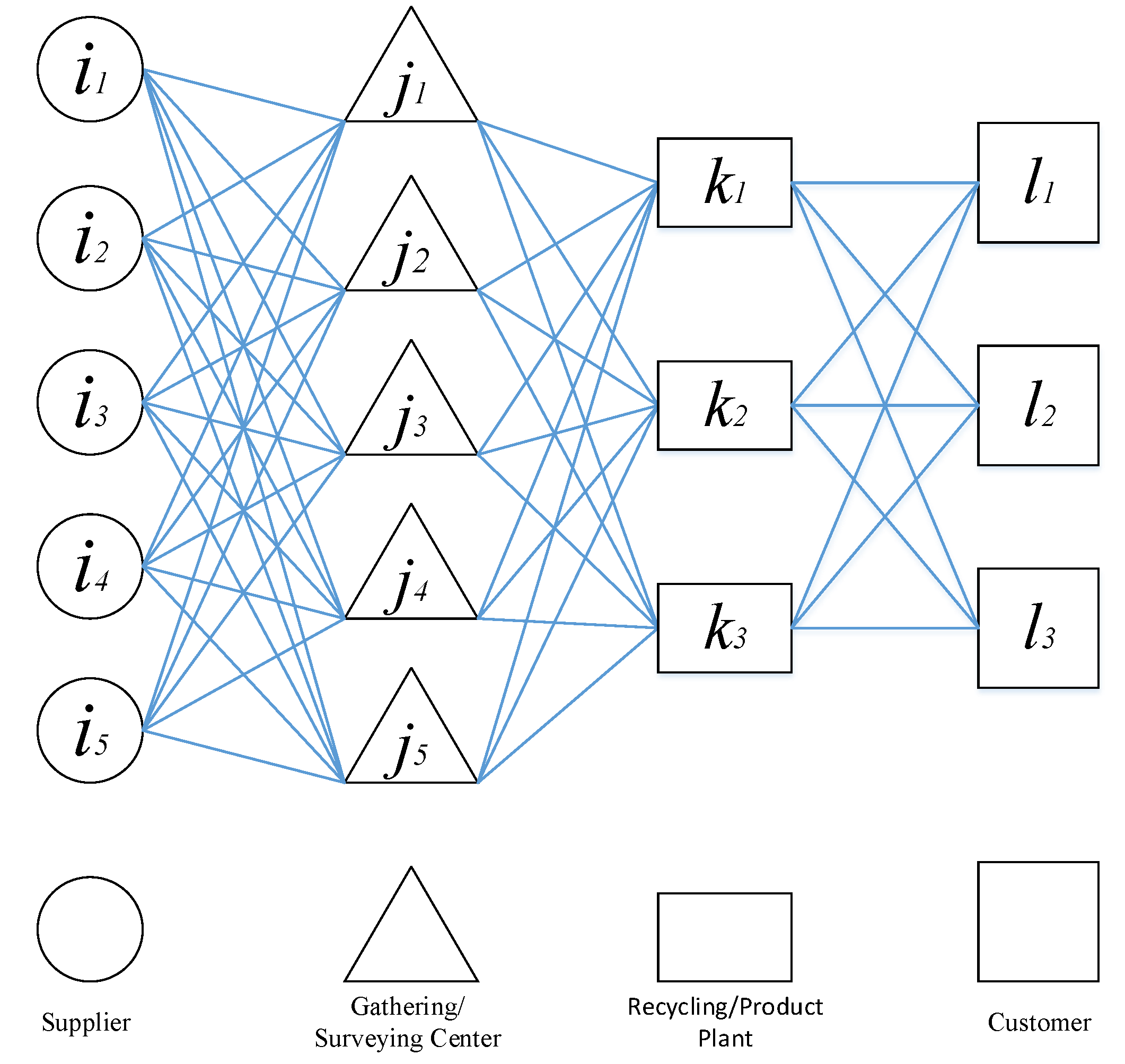
In this research, scenario planning was used to deal with uncertainty in the demand parameter due to unpredictable changes that have occurred during the research period in the studied case. To realize the economic, environmental and social effects of the reverse SCN and to optimize the model, three objectives were laid out, including maximizing operating profit, minimizing adverse environmental impacts and maximizing the level of service to suppliers and customers. To consider uncertainty, the multi-echelon supply chain, reverse logistics, and green supply design, the logistics network presented in this study consisted of four levels. The first level was the waste providers, considered as returning product suppliers, which could be the customers of previous periods who have returned their remaining products or can be new suppliers of scrap supplies. The second level was the gathering centers of the returned products, being responsible for supplying the scrap from the first-level suppliers of the chain, and in particular, being responsible for supplying the returned product, inspection, sorting, storage, and transferring the product to the recycling plants (product factories). The third level was the recycling plants for the production of new products, based on the received scrap from the gathering centers, which were responsible for producing new products. Finally, the fourth level was the customers. According to the given explanation, the proposed network is shown as a framework in Figure 1.

The overall aim of this study was to design a sustainable reverse logistics integrated model in conditions of demand uncertainty, to optimize the flow of materials throughout the SC, and to determine the number and location of facilities and the planning of SC transportation. In this regard, the following objectives were considered in this research:

• Identifying and categorizing the necessary processes to implement the reverse logistics network of the steel industry;
• Maximizing the operating profit of the SC so as to meet economic requirements;
• Minimizing the adverse environmental impacts to meet environmental requirements;
• Maximizing the satisfaction of suppliers and customers to meet social requirements.

This study presents a multi-objective mathematical model for reverse SC design. The proposed model allows the NSGA-II algorithm to plan the recycling of products in the Iranian steel industry based on the modified approach of Feito Cespon et al. (2017) with their model. The proposed model has the following features [22]:

• Using a robust optimization approach and NSGA-II algorithm for the multi-objective modeling of the reverse SCN, including the flows of materials and transportation planning in conditions of uncertain demand;
• Evaluating environmental indicators based on CO₂ emissions as one of the most important greenhouse gas emissions in the environment;
• Evaluating customer service levels (CSLs) based on maximizing the received products returned from suppliers/previous customers and selling new products to customers;
• Defining different scenarios for dealing with uncertainty of demand and quantifying them according to expert opinion.

A reverse logistics network as part of the SC means the accurate, correct and timely transmission of materials and the types of goods that are usable and unusable from the endpoint (last consumer or end-user) through the SC to the appropriate plant. In this regard, many types of research have been previously illustrated.

Table 1. Previous related research.

Solution Method	Network Flow		Network Design					Attributes of the Mathematical Model				Objective Function			Researcher
	Reverse	Forward	Collecting and Distribution	Transport	Facilities	Repair and Recovery	Recycling	Limited Capacity	Multi-Period	Multi-Product	Uncertainty	Customer Service Level	Environmental Issues	Minimizing the Cost
Mathematical Programming		✓				✓					✓			✓	[23]
New Optimization Model	✓					✓	✓		✓				✓		[24]
Mathematical Programming and Goal Programming Technique		✓					✓		✓				✓	✓	[25]
Genetic Algorithm		✓		✓										✓	[26]
Multi-Objective Programming		✓		✓									✓	✓	[27]
Metaheuristic Method		✓	✓	✓									✓	✓	[28]
Multi-Objective Linear Fuzzy Programming		✓									✓		✓	✓	[29]
Multi-Objective Genetic Algorithm		✓	✓			✓			✓			✓	✓	✓	[30]
Fuzzy Optimization		✓							✓	✓	✓			✓	[31]
Mixed Integer Nonlinear Programming Model	✓	✓	✓		✓					✓	✓			✓	[32]
Column Generation Paradigm	✓		✓		✓	✓	✓			✓				✓	[33]
Robust Optimization	✓			✓			✓				✓		✓	✓	[22]
Mathematical Programming	✓				✓					✓		✓	✓	✓	[34]
Two-Stage Stochastic Programming		✓			✓					✓	✓			✓	[20]
Mathematical Programming and Lagrange Algorithm	✓					✓			✓		✓			✓	[35]
Mathematical Programming	✓							✓		✓		✓	✓	✓	[36]
Complex Integer Nonlinear Programming, HGA and HHS	✓										✓	✓		✓	[37]
Single Objective Programming, Genetic and Neighborhood Search		✓						✓						✓	[38]
Mathematical Programming	✓			✓			✓				✓			✓	[39]
Mathematical Programming	✓				✓					✓		✓	✓	✓	[40]
Mathematical Programming, Two-Phase Stochastic Programming		✓		✓	✓			✓			✓			✓	[41]
Mathematical Programming, Lp-Metric Based Method	✓	✓	✓		✓	✓		✓	✓	✓		✓	✓	✓	[42]
Multi-Objective		✓	✓	✓						✓	✓		✓	✓	[43]
Queueing Network Model	✓	✓	✓		✓					✓	✓		✓	✓	[44]
De Novo Programming Method	✓	✓	✓	✓		✓				✓		✓		✓	[45]
Robust Optimization	✓	✓	✓	✓			✓	✓		✓	✓		✓	✓	Current Study

compares the illustrated pieces of research with the proposed method, from different perspectives.

According to previous research, although many studies and articles have focused on the issue of sustainable SCN, there are some knowledge gaps in this area that are briefly summarized as follows:

• Most research focuses on the design of a new SC, and there exists a shortage of network redesign;
• The impact of the number and location of facilities on the environment is not considered;
• There are very few models that consider reconstructing reverse SC with a simultaneous analysis of social, economic, and environmental goals;
• Uncertainty about the number of resources and demand for recycled products, along with the management of diverse materials, are issues that require investigation in the future.

Based on the above-mentioned gaps, the present study expresses a multi-objective mathematical model for redesigning the reverse SC network. The proposed model allows the use of a robustness approach to recycling multiple products. The proposed model has the following features:

• The use of a robust optimization approach for redesigning a recycling SC network, including multiple flows of materials and uncertainties regarding the waste products used as raw materials, and the final demand for recycled products;
• The structure of the expected functional index for evaluating a configuration for a new SC considering the economic and environmental objectives in different scenarios.

2. Methods and Materials

Based on the above mentioned theoretical background and defined problem, to resolve the uncertainty of the model parameters, a scenario-based robust optimization by the augmented epsilon constraint method was developed using the General Algebraic Modeling System (GAMS) software. An augmented epsilon constraint method was used for cases of multi-objective optimization in which one of the objective functions was more important than the other functions, and based on this, the optimization of other functions was performed. In this study, due to the greater importance of the first objective function compared to the others, this method was used. Since the main model with the network and the actual data of the case study by the GAMS cannot be solved, the objectives were defined based on an initial model on a smaller scale; they were solved by a scenario-based robust optimization, and the comparison and validation of the model were investigated by the NSGA-II algorithm in MATLAB.

2.1. Assumptions

• Uncertainty in the demand parameter has been considered;
• The studied SC consists of four levels when acting in a single period;
• The capacity of the gathering centers is unlimited, and the capacity of the recycling plants is limited;
• The numbers of gathering centers and recycling plant candidates are limited;
• Fixed and variable costs (gathering, recycling and transportation) and the number and capacity of the transportation modes are determined;
• The flow of material between two non-consecutive levels is not allowed;
• The numbers of suppliers and customers are fixed and are five and three, respectively;
• The nominated locations for selecting gathering centers and recycling plants are five and three, respectively. These will determine the exact number of centers during the process of solving the model [22].

2.2. Model Notations

Based on the SC structure shown in Figure 1, the problem is formulated as a multi-objective optimization model. The list of indices, parameters and decision variables of the model are presented in this section. This proposed model is based upon the work of Feito Cespon et al. 2017 [22] by using different objective functions, and case study and solving approaches, to compare the results.

The notations used in the paper are as follows.

Indexes

$i\in I$	A set of renewable waste suppliers
$j\in J$	A set of location candidates for gathering centers
$k\in K$	A set of location candidates for recycling plants
$l\in L$	A set of customers
$m\in M$	A set of transportation modes
$p\in P$	A set of final products
$s\in S$	A set of scenarios

Parameters

Gip	The amount of product supply (p) by the supplier (i), in tons per month
CTmp	The capacity of the transportation mode (m) for the transfer of product (p), in tons, on the trip
Ckp	The capacity of the recycling plant (k) to produce the product (p), in tons per month
Dlps	The amount of product (p) which is demanded by the customer (l) under the scenario (s), in tons per month
NVm	Total number of trips available for each mode (m)
ITm	The environmental impact of moving materials in the transportation mode (m) on the environmental index, per ton-km
IE	The environmental effect of the total gas consumption of the system on the environmental index, per normal cubic meter per hour
IP	The environmental impact of infrastructure in the environmental index
IA	The environmental impact generated by water consumption on the whole system in the environmental index, per cubic meter
Cfek	Stable gas consumption at the recycling plant (k) in relation to normal condtions, in cubic meters per hour
Cfej	Fixed gas consumption of the gathering center (j) in normal conditions, in cubic meters per hour
Cvep	Variable gas consumption to produce a unit of product (p) in normal conditions, in cubic meters per hour
Cvap	Variable water consumption to obtain a unit of product (p), in cubic meters
${\alpha }_k·{\beta }_j$	Gathering center (j) and recycling plant (k) capacity ratio
$d_{ij}^{SR}$	Distance between supplier (i) and the gathering center (j), in km
$d_{jk}^{RP}$	Distance between gathering center (j) and recycling plant (k), in km
$d_{kl}^{PC}$	Distance between recycling plant (k) and customer (l), in km
CURjp	The cost of production (p) in the gathering center (j), in rials per ton
CUPkp	The cost of production (p) in the recycling plant (k), in rials per ton
CUTm	The variable cost of the transport mode (m), in rials per km
CFRj	Fixed cost of using the gathering center (j), in rials
CFPk	Fixed cost of using a recycling plant (k), in rials
PSs	Probability of scenario (s)
PRIp	Product sales price (p)

Variables

QSRijmps	The amount of product supply (p) that is transmitted in the transportation mode (m) between the waste supplier (i) and the gathering center (j) under the scenario (s), in tons
QRPjkmps	The amount of product (p) that is transmitted in the transportation mode (m) between the gathering center (j) and the recycling plant (k) under the scenario (s), in tons
QPCklmps	The amount of product (p) transmitted in the transportation mode (m) between the recycling plant (k) and customer (l) under the scenario (s), in tons
VSRijms	The number of trips between the waste supplier (i) and the gathering center (j) using the transportation mode (m) under the scenario (s)
VRPjkms	The number of trips between the gathering center (j) and the recycling plant (k) using the transportation mode (m) under the scenario (s)
VPCklms	The number of trips between the recycling plant (k) to the customer (l) using the transportation mode (m) under the scenario (s)
HSRijms HRPjkms HPCklms	Variables that indicate the number of trips (excess or defect) to balance between the transportation modes
Rj	Variable; 1 if the gathering center (j) is used, otherwise it is zero
Pk	Variable; 1 if the recycling plant (k) is used, otherwise it is zero

2.3. Model Objective Functions

Equation (1) maximizes the operating profit of the SC.

$$\begin{array}{ll}\max {{\displaystyle f}}_1& ={\displaystyle \sum _s{{\displaystyle PS}}_s({\displaystyle \sum _k{\displaystyle \sum _p{{\displaystyle PRI}}_p}{\displaystyle \sum _l{\displaystyle \sum _m{{\displaystyle QPC}}_{klmps}}}}}\\ & {{\displaystyle }}_{}^{}{{\displaystyle }}_{}^{}{{\displaystyle }}_{}^{}-({\displaystyle \sum _m{{\displaystyle CUT}}_m·}({\displaystyle \sum _j{\displaystyle \sum _k{{\displaystyle VRP}}_{jkms}{{\displaystyle d}}_{jk}^{PC}}}\\ & {{\displaystyle }}_{}^{}{{\displaystyle }}_{}^{}{{\displaystyle }}_{}^{}+{\displaystyle \sum _k{\displaystyle \sum _l{{\displaystyle VPC}}_{klms}{{\displaystyle d}}_{kl}^{PC}}}\\ & {{\displaystyle }}_{}^{}{{\displaystyle }}_{}^{}{{\displaystyle }}_{}^{}+{\displaystyle \sum _i{\displaystyle \sum _j{{\displaystyle VSR}}_{ijms}{{\displaystyle d}}_{ij}^{SR}}}))\\ & {{\displaystyle }}_{}^{}{{\displaystyle }}_{}^{}{{\displaystyle }}_{}^{}-{\displaystyle \sum _k{{\displaystyle CFP}}_k{{\displaystyle P}}_k-{\displaystyle \sum _k{\displaystyle \sum _p{{\displaystyle CUP}}_{kp}{\displaystyle \sum _l{\displaystyle \sum _m{{\displaystyle QPC}}_{klmps}}}}}}\\ & {{\displaystyle }}_{}^{}{{\displaystyle }}_{}^{}{{\displaystyle }}_{}^{}-{\displaystyle \sum _j{{\displaystyle CFR}}_j{{\displaystyle R}}_j-{\displaystyle \sum _j{\displaystyle \sum _p{{\displaystyle CUR}}_{jp}{\displaystyle \sum _k{\displaystyle \sum _m{{\displaystyle QRP}}_{jkmps}}}}}}\end{array}$$

(1)

Equation (2) minimizes the adverse environmental impacts of the SC.

$$\begin{array}{ll}\min {{\displaystyle f}}_2& ={\displaystyle \sum _{s}P{S}_s}(\\ & {{\displaystyle }}_{}^{}{{\displaystyle }}_{}^{}{{\displaystyle }}_{}^{}{\displaystyle \sum _{m}I{T}_m}({\displaystyle \sum _i{\displaystyle \sum _j{\displaystyle \sum _p{{\displaystyle QSR}}_{ijmps}}{{\displaystyle d}}_{ij}^{SR}}}\\ & {{\displaystyle }}_{}^{}{{\displaystyle }}_{}^{}{{\displaystyle }}_{}^{}+{\displaystyle \sum _j{\displaystyle \sum _k{\displaystyle \sum _p{{\displaystyle QRP}}_{jkmps}}{{\displaystyle d}}_{jk}^{RP}}}\\ & {{\displaystyle }}_{}^{}{{\displaystyle }}_{}^{}{{\displaystyle }}_{}^{}+{\displaystyle \sum _k{\displaystyle \sum _l{\displaystyle \sum _p{{\displaystyle QPC}}_{klmps}}{{\displaystyle d}}_{kl}^{PC}}})\\ & {{\displaystyle }}_{}^{}{{\displaystyle }}_{}^{}{{\displaystyle }}_{}^{}+IE({\displaystyle \sum _k{{\displaystyle Cfe}}_k{{\displaystyle P}}_k}+{\displaystyle \sum _j{{\displaystyle Cfe}}_j{{\displaystyle R}}_j+{\displaystyle \sum _p{{\displaystyle Cve}}_p{\displaystyle \sum _k{\displaystyle \sum _l{\displaystyle \sum _m{{\displaystyle QPC}}_{klmps})}}}}}\\ & {{\displaystyle }}_{}^{}{{\displaystyle }}_{}^{}{{\displaystyle }}_{}^{}+IP({\displaystyle \sum _k{{\displaystyle \alpha }}_k{{\displaystyle P}}_k+{\displaystyle \sum _j{{\displaystyle \beta }}_j{{\displaystyle R}}_j)+IA{\displaystyle \sum _p{{\displaystyle Cva}}_p{\displaystyle \sum _k{\displaystyle \sum _l{\displaystyle \sum _m{{\displaystyle QPC}}_{klmps}}}}}}})\\ & {{\displaystyle }}_{}^{}{{\displaystyle }}_{}^{}{{\displaystyle }}_{}^{}\end{array}$$

(2)

Equation (3) maximizes the supplier’s and customers’ service levels, being different from that in the work of Feito Cespon et al. 2017 [22]:

$$\max {{\displaystyle f}}_3={\displaystyle \sum _s{P}_s}(\frac{\left[{\displaystyle \sum _k{\displaystyle \sum _l{\displaystyle \sum _m{\displaystyle \sum _p{{\displaystyle QPC}}_{klmps}}}}}+{\displaystyle \sum _i{\displaystyle \sum _j{\displaystyle \sum _m{\displaystyle \sum _p{{\displaystyle QSR}}_{ijmps}}}}}\right]}{\left[{\displaystyle \sum _l{\displaystyle \sum _p{{\displaystyle D}}_{lps}}}+{\displaystyle \sum _i{\displaystyle \sum _p{{\displaystyle G}}_{ip}}}\right]})$$

(3)

2.4. Model Constraints

The model constraints are shown in Equations (4) to (19). Each constraint has been discussed below [22]:

• Equations (4) to (6) guarantee the flow of materials through the SCN. The output from each center is, at most, equal to the inputs from different centers at the previous level of the SC;

  $${\displaystyle \sum _j{\displaystyle \sum _m{{\displaystyle QSR}}_{ijmps}\le {{\displaystyle G}}_{ip}}}\hspace{1em}\forall i,p,s$$

  (4)

  $${\displaystyle \sum _k{\displaystyle \sum _m{{\displaystyle QRP}}_{jkmps}\le {\displaystyle \sum _i{\displaystyle \sum _m{{\displaystyle QSR}}_{ijmps}}}}}\hspace{1em}\forall j,p,s$$

  (5)

  $${\displaystyle \sum _l{\displaystyle \sum _m{{\displaystyle QPC}}_{klmps}\le {\displaystyle \sum _j{\displaystyle \sum _m}}}}{{\displaystyle QRP}}_{jkmps}\hspace{1em}\forall k,p,s$$

  (6)

• Equations (7) and (8) respectively guarantee that the flow of materials rate does not exceed the maximum capacity of the recycling plants and the product demand;

  $${\displaystyle \sum _l{\displaystyle \sum _m{{\displaystyle QPC}}_{klmps}\le {{\displaystyle C}}_{kp}}}\hspace{1em}\forall k,p,s$$

  (7)

  $${\displaystyle \sum _k{\displaystyle \sum _m{{\displaystyle QPC}}_{klmps}\le {{\displaystyle D}}_{lps}}}\hspace{1em}\forall l,p,s$$

  (8)

• Equations (9) to (11) maintain the balance between two facilities concerning the number of transportation. Since the number of transport must be an integer value, a series of inactive variables have been suggested to maintain the model’s probability;

  $${\displaystyle \sum _p\frac{{{\displaystyle QSR}}_{ijmps}}{{{\displaystyle CT}}_{mp}}+{{\displaystyle HSR}}_{ijms}={{\displaystyle VSR}}_{ijms}}\hspace{1em}\forall i,j,m,s$$

  (9)

  $${\displaystyle \sum _p\frac{{{\displaystyle QRP}}_{jkmps}}{{{\displaystyle CT}}_{mp}}+{{\displaystyle HRP}}_{jkms}={{\displaystyle VRP}}_{jkms}}\hspace{1em}\forall j,k,m,s$$

  (10)

  $${\displaystyle \sum _p\frac{{{\displaystyle QPC}}_{klmps}}{{{\displaystyle CT}}_{mp}}+{{\displaystyle HPC}}_{klms}={{\displaystyle VPC}}_{klms}}\hspace{1em}\forall k,l,m,s$$

  (11)

• Equations (12) to (14) guarantee that ineffective variables focus only on differences in the number of transport;

  $${{\displaystyle VSR}}_{ijms}+{{\displaystyle HSR}}_{ijms}\ge 0 \begin{array}{l}\forall i,j,m,s,\\ (-1<{{\displaystyle HSR}}_{ijms}<1)\end{array}$$

  (12)

  $${{\displaystyle VRP}}_{jkms}+{{\displaystyle HRP}}_{jkms}\ge 0 \begin{array}{l}\forall j,k,m,s,\\ (-1<{{\displaystyle HRP}}_{jkms}<1)\end{array}$$

  (13)

  $${{\displaystyle VPC}}_{klms}+{{\displaystyle HPC}}_{klms}\ge 0 \begin{array}{l}\forall k,l,m,s,\\ (-1<{{\displaystyle HPC}}_{klm}<1)\end{array}$$

  (14)

• Equation (15) limits the number of trips per transportation mode [21];

  $${\displaystyle \sum _i{\displaystyle \sum _j{{\displaystyle VSR}}_{ijms}+{\displaystyle \sum _j{\displaystyle \sum _k{{\displaystyle VRP}}_{jkms}}}+{\displaystyle \sum _k{\displaystyle \sum _l{{\displaystyle VPC}}_{klms}\le {{\displaystyle NV}}_m}}}}\hspace{1em}\forall m,s$$

  (15)

• According to Equations (16) and (17), binary variables should be assumed, such that if a gathering center or recycling plant is used in the model, then the value is 1, and otherwise it is zero;

  $${\displaystyle \sum _k{\displaystyle \sum _m{\displaystyle \sum _p{{\displaystyle QRP}}_{jkmps}\le M{R}_j}}}\hspace{1em}\forall j,s$$

  (16)

  $${\displaystyle \sum _l{\displaystyle \sum _m{\displaystyle \sum _p{{\displaystyle QPC}}_{klmps}\le M{{\displaystyle P}}_k}}}\hspace{1em}\forall k,s$$

  (17)

• Finally, Equations (18) and (19) show the nature of the variables.

  $$\begin{array}{l}{{\displaystyle QRP}}_{jkmps},{{\displaystyle QPC}}_{klmps},{{\displaystyle QSR}}_{ijmps},{{\displaystyle VPC}}_{klms},\\ {{\displaystyle VRP}}_{jkms},{{\displaystyle VSR}}_{ijms}\ge 0\end{array}$$

  (18)

  $${{\displaystyle R}}_j,{{\displaystyle P}}_k\in \{0,1\}$$

  (19)

3. Results

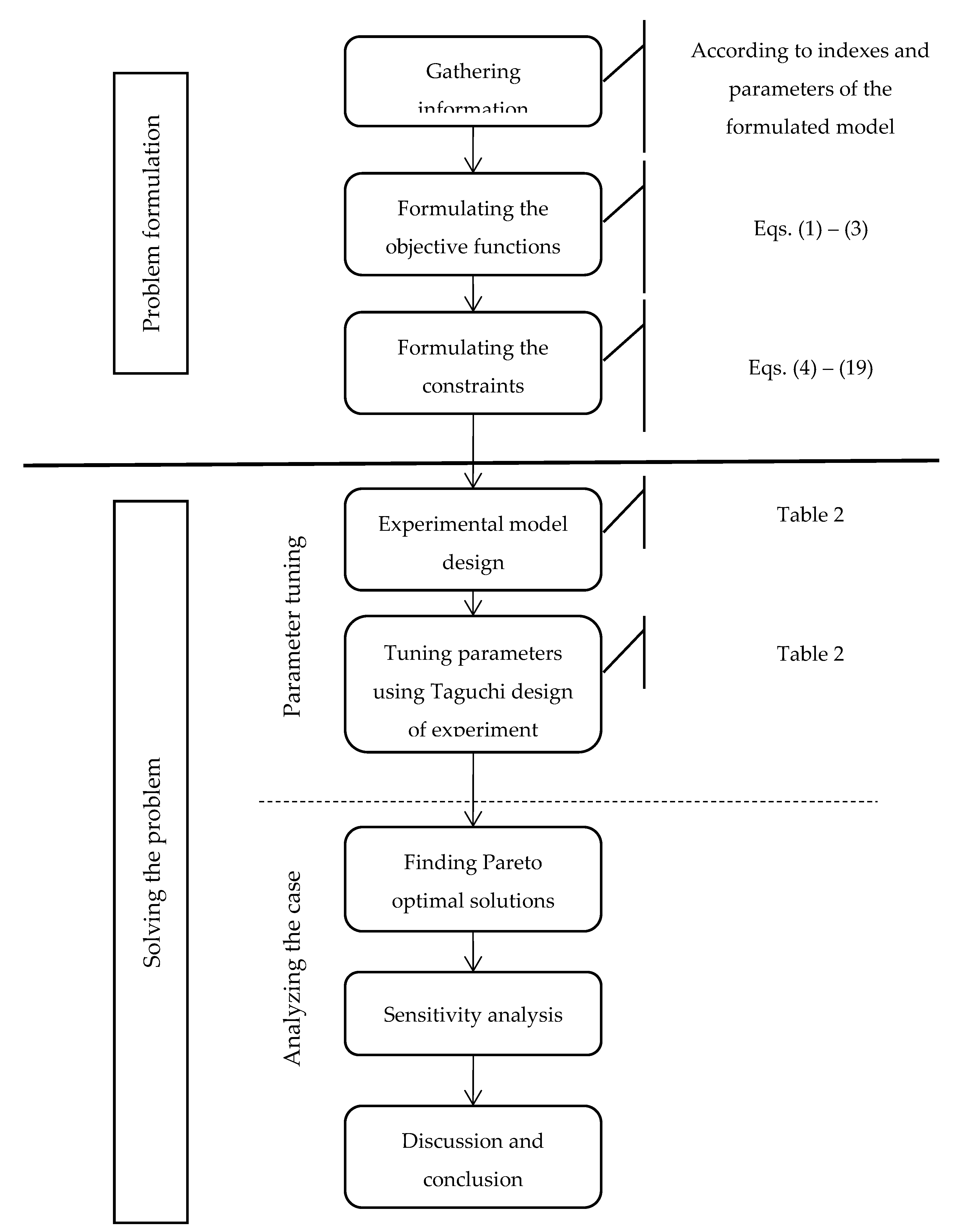
This proposed model is based upon the work of Feito Cespon et al. 2017 [22] by using a different objective function and case study and different solving approaches to compare the results. This is due to the main model (real-world case study) not being solvable with mathematical programming methods. At first, a smaller scale research model with fewer data called the “Initial Model” can be solved by an augmented epsilon constraint method, and subsequently, it is solved by the NSGA-II algorithm [46,47]. Furthermore, the performance of the NSGA-II algorithm is evaluated by solving several examples in the proposed research model, and the corresponding criteria are calculated. Afterwards, with the confidence of the model’s validity, and since the main problem is Np-hard, the model of the real-world case study called “Main Model” is solved by the NSGA-II algorithm and will be analyzed at the end. Note that sensitivity analysis will be implemented on the initial model. Before solving the model, the method for determining the chromosome in the NSGA-II algorithm is presented. The algorithmic scheme of this section is illustrated in Figure 2.

3.1. Definition of Chromosomes in the NSGA-II Algorithm

The matrix of the answer in the model has two sections, called allocation and assignment. The allocation section has two parts, the first part of which is the location of the gathering centers (J), and the second part is the location of the recycling plants (K). The cells of the matrix are filled with numbers 0 or 1, for example, if J = 5 and K = 3; an example of this matrix is given in Table 2.

According to Table 2, gathering center No. 5 has been constructed, and gathering centers No. 1, 2, 3 and 4 have not been constructed. Moreover, the recycling plant No.1 has been constructed and the recycling centers No. 2 and 3 have not been constructed. Each set is the answer that is called a chromosome. The assignment section shows the flow rate from the waste supplier to the gathering centers, from the gathering centers to the recycling plants and from the recycling plants to the customers. In Table 3, the assignment section is shown. As a case in point, in the first part of the following table, which is a K ∗ L dimensional matrix, the flow rates from the recycling plants (k) to the customer (l) for the transportation mode (m), that is m = 1, p = 1 and s = 1, are shown.

Based on Table 3, it is obvious that the flow rate of product 1 from the recycling plant 1 to customer 1 by transportation mode 1 in scenario 1 is 3. In this regard, each answer set is called a chromosome, and each cell is a gene.

3.2. NSGA-II Operator Selection

Achieving a high performance of genetic algorithms is highly dependent on the performance of the genetic operators. One of the main operators in genetic algorithms is crossover. The crossover operator is used to generate a new chromosome by crossing over two selected chromosomes. Different crossover operators are represented in previous studies. Here in this paper, the single point crossover is used. The next important operator is a mutation to assure diversity. Beyond the mutation probability that is tuned in Section 3.6, in this study, the reverse and replace operators are used randomly to mutate the selected chromosomes. In reverse mutation, two genes are selected in the considered chromosome, and the values of remaining genes between these two selected genes are reversed from right to left. In the replacement mutation, two genes are selected, and their positions are swapped with one another’s.

3.3. Initial Model Solving Results

Table 4. The specifications and parameters of the initial model.

Number of Suppliers	2	Number of Gathering Center	2	Number of products	2
umber of Recycling Plant	2	Number of Customers	2
Number of Transportation modes	2	Number of Scenarios	2

indicates SC characteristics in the initial model. Furthermore, the probability of the occurrence of each scenario is obtained using the analytical hierarchical process (hereafter AHP) method, which for scenarios 1 to 2, is 52.4% and 47.6%, respectively. Moreover, in the initial model, a big M value is 10,000.

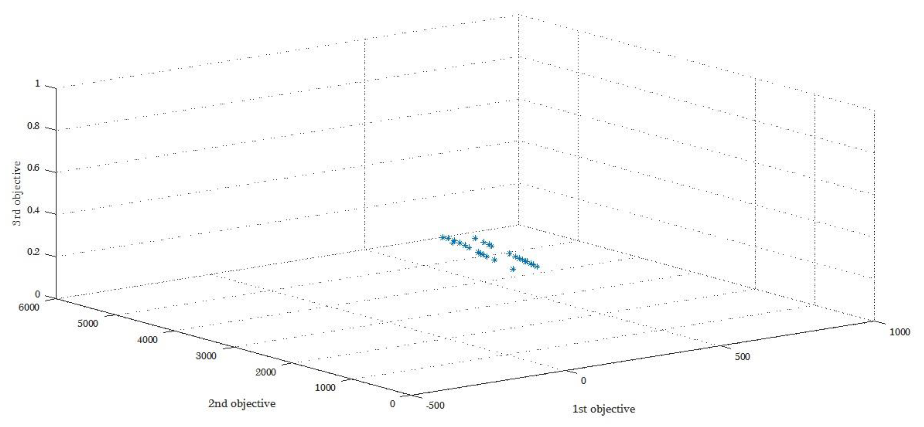
The Pareto result according to the GAMS and NSGA-II algorithm of five sets of answers derived from the initial model solving is shown in

Table 5. Pareto points set by the GAMS for the initial model.

Answer No.	The Value of the First Objective Function	The Value of the Second Objective Function	The Value of the Third Objective Function
1	−128.17	2271.64	0.8
2	−247.05	1135.82	0.6
3	−92.47	801.17	0.41
4	67.78	1135.82	0.2
5	87.77	2271.64	0.6

and

Table 6. Pareto points set by the NSGA-II algorithm for the initial model.

Answer No.	The Value of the First Objective Function	The Value of the Second Objective Function	The Value of the Third Objective Function
1	−21.51	1961.65	0.4876
2	−8.1	1944.2	0.4819
3	3.65	1920.59	0.46
4	3.85	1896.37	0.4706
5	13.4	1860.68	0.4607

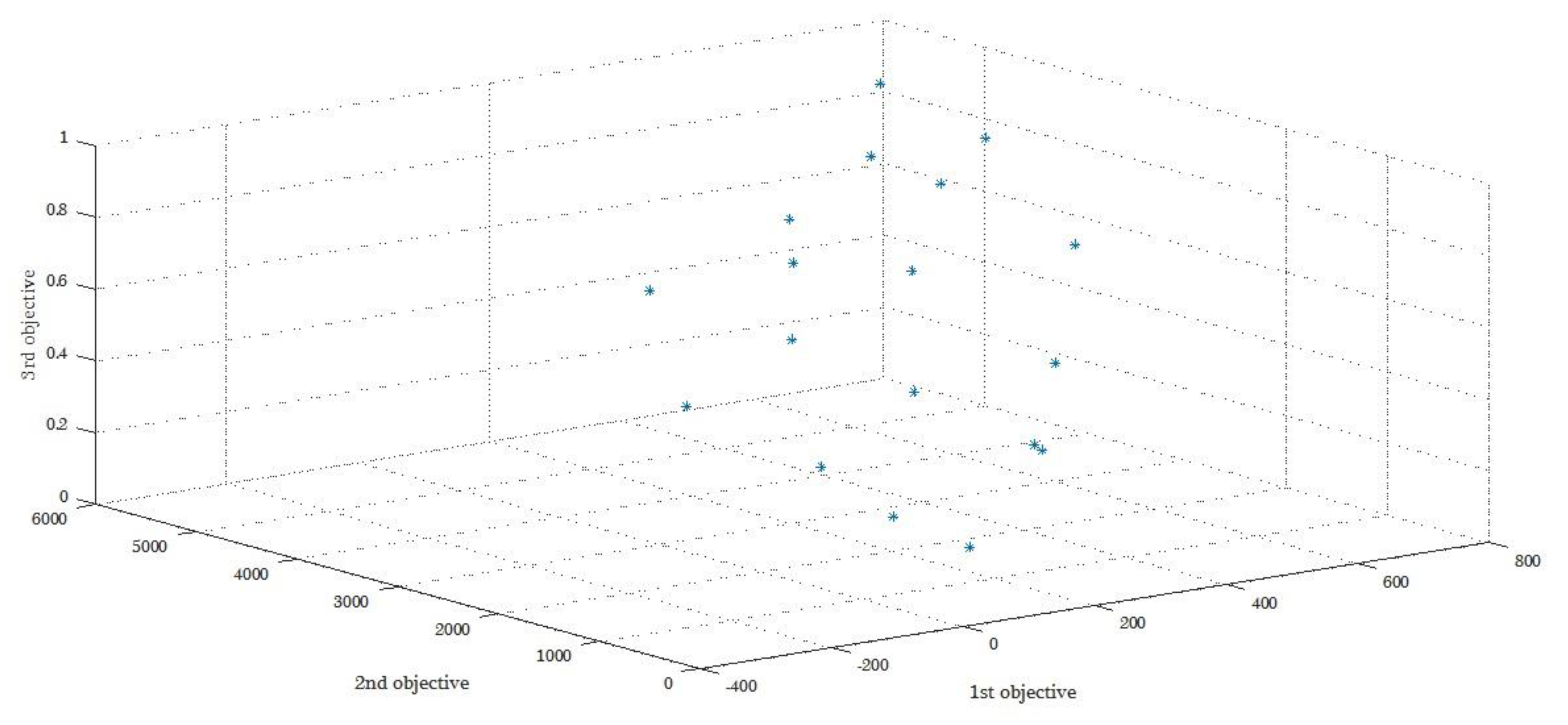
. Figure 3 and Figure 4 show these Pareto points. It is conceivable that the results obtained for the small scale problems by GAMS will outperform the NSGA-II results, as this can be seen in similar studies [48,49,50]; however, as it is illustrated in the next sections, the main advantage of NSGA-II is in its ability to solve large scale and real-world problems. The time of the GAMS solving in this model, although the problem dimensions are low, is 326 seconds, which is increased sharply by increasing the dimensions of the problem.

Figure 3 and Figure 4 show that when the values of the first objective function deteriorate, the values of the other objectives function do not. In other words, these values remain either constant or close to their optimal values, which is the expected process that the multi-objective models suggest.

3.4. Model Validation

To evaluate the performance of the model and to compare the performance of the NSGA-II algorithm with the augmented epsilon constraint method, five examples with different dimensions randomly compiled on the research model, and the criteria for comparing the efficiency of the multi-objective algorithms, are calculated, the results of which are shown in

Table 7. Comparison of indices for five examples with NSGA-II algorithms and the Epsilon Constraint method.

Item	Epsilon Constraint					NSGA-II
	MID	Spacing	Diversity	NoS	Time(s)	MID	Spacing	Diversity	NoS	Time(s)
1	8556.59	51.73	2562.22	14	8	7283.27	13.05	2858.35	96	55.96
2	7574.8	73.37	3820.57	16	13	7749.36	79.91	2247.99	97	63.73
3	5383.46	181.73	6709.34	23	48	6720.7	30.82	3616.23	98	58.43
4	6317.78	181.41	5209.74	16	93	7150.89	28.77	2423.52	99	57.68
5	7109.71	242.98	5219.62	18	407	7903.34	13.88	1650.52	95	58.53

. The results are obtained by running the proposed algorithm in a single trial with a population size of 10,000 and 250 repetitions. As the results indicate, it can be seen that using the NSGA-II algorithm has the necessary validity to solve the main model.

In this table, five measures are reported. Mean Idear Distance (MID) measures the convergence of an algorithm by averaging the distances of solutions from the best feasible solution [51,52]. Spacing measures the standard deviation of the distances among the Pareto front solution [52]. Diversity evaluates the spread of the Pareto front [52]. The Number of solutions (NoS) is the number of different Pareto solutions [53,54]. Time(s) is the time for which the algorithm needs to be run to reach the near-optimal solution [53,54].

The lower the index MID, the better the research results. As can be seen, the performance of the Epsilon Constraint (E.C). method in two sets of responses is better than that of the NSGA-II algorithm; however, with increasing dimensions of the problem, the method of E.C. loses its effectiveness. Since this difference is not very high, both indicators have shown good performance.

The lower the index spacing, the better the research results. According to Table 7, the performance of the NSGA-II algorithm is better than that of the E.C. method. The higher the index (diversity), the better the research results. Based on the results, it can be seen that the proposed E.C method is better than the NSGA-II algorithm.

The higher the index NoS, the better the research results. Based on the results, the NSGA-II algorithm obtained a greater number of Pareto members. It is logical to increase the solution time of the algorithms by increasing the dimensions of the problem.

Therefore, according to the results, the same trend is observed; with an increase in the dimensions of the problems, the time taken to solve by the method of E.C. increases exponentially, and this method loses its efficiency in high-dimensional issues. However, it is almost constant for the NSGA-II algorithm.

3.5. The Parameter Adjustment of the NSGA-II Algorithm

Under the meta-heuristic algorithms that do not guarantee an exact optimal solution, the algorithm may be followed by a different response at any time by solving it. Therefore, a meta-heuristic algorithm is good when used, with almost identical answers each time. The most influential parameters in the NSGA-II algorithm are the number of initial population (nPop), the number of repetitions (MaxIt), the intersection rate (Pc) and the rate of mutation (Pm). With using the Taguchi design of experiments method, the parameters of this algorithm are based on comparative criteria for nine exams that have been determined under the following steps.

3.6. Taguchi Design of Experiment

In the NSGA-II algorithm, the four factors/parameters MaxIt, nPop, Pc, and Pm should be set to optimal levels. For this purpose, at first, for each parameter, three levels of low (1), medium (2) and high (3) are considered, as shown in

Table 8. The setting up NSGA-II parameters at three levels.

NSGA-II Parameters	Low Level (1)	Middle Level (2)	High Level (3)
MaxIt	60	80	100
nPop	50	70	100
Pc	0.7	0.8	0.9
Pm	0.15	0.25	0.35

. The proposed Taguchi experiments for four factors at three levels are shown in

Table 9. Taguchi designed experiments to adjust the parameters of the NSGA-II algorithm.

Exam No.	MaxIt	nPop	Pc	Pm
1	1	1	1	1
2	1	2	2	2
3	1	3	3	3
4	2	1	2	3
5	2	2	3	1
6	2	3	1	2
7	3	1	3	2
8	3	2	1	3
9	3	3	2	1

for nine experiments. These experiments are designed based on Taguchi methods [55].

Table 8 reveals the levels of the NSGA-II parameters, for each parameter considering three different levels. Table 9 demonstrates the experiments designed to adjust the parameters of the NSGA-II algorithm. In

Table 10. Results from the experiments of the NSGA-II algorithm.

No.	MID	Spacing	Diversity	NoS	Time(s)
1	7636.4	23.4	1869.3	50	27.4
2	7725.7	19.6	2329.9	68	48.4
3	7677.5	22.4	2453.4	100	130.4
4	7745.1	70.8	2677.1	49	42.7
5	7615.1	58.1	3041.4	69	69.5
6	7801.7	91.8	3019.3	97	125.9
7	7640.1	32.1	1924.5	48	48.7
8	7670.5	39.2	2856.5	70	85.5
9	7678.4	30.6	2598.7	98	152.9

, the results of the NSGA-II algorithm for nine independent experiments are presented.

According to Table 10, to create an output from each test and for five criteria, using the fuzzy unambiguous technique and the ideal planning approach, all indicators become responses after normalization. The normalization of the results and the calculation of the response variable are shown in

Table 11. Normalized results and the calculation of responses for setting the parameter of the NSGA-II algorithm.

No.	MID	Spacing	Diversity	Nos	Time(s)	Response
1	0. 11	0.05	1.00	0.96	0.00	22.46
2	0.59	0.00	0.61	0.62	0.17	65.89
3	0.33	0.04	0.5	0.00	0.82	39.22
4	0.7	0.71	0.31	0.98	0.12	81.30
5	0.00	0.53	0.00	0.6	0.34	6.24
6	1.00	1.00	0.02	0.06	0.79	111.05
7	0.13	0.17	0.95	1.00	0.17	25.37
8	0.3	0.26	0.16	0.58	0.46	35.24
9	0.34	0.15	0.38	0.04	1.00	40.34

.

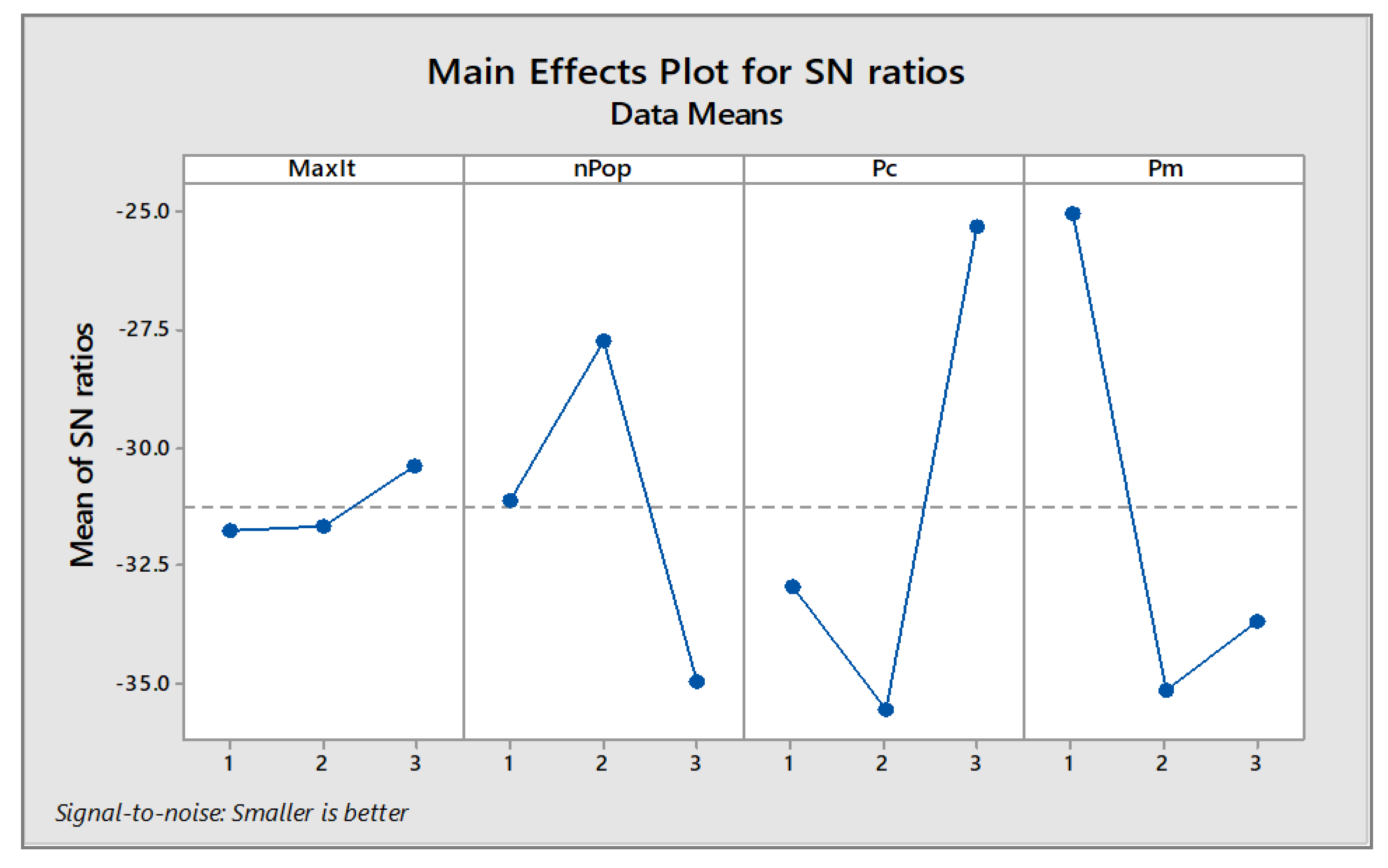
In the last step, based on the calculated response variable in the previous step, the S/N rate is calculated, and the optimal levels of the input parameters are determined. This operation is performed by the MINITAB software, and the results are illustrated in Figure 5. This figure illustrates the main effect plot of different algorithm parameters. The plots are plotted by fixing parameters at their three levels, and then comparing the means of the S/N ratios against those at different levels.

The optimal levels for the parameters of the algorithm examined according to Figure 5 and the above tables are shown in

Table 12. Optimized levels for the NSGA-II algorithm.

	MaxIt	nPop	Pc	Pm
NSGA-II	Level 3	Level 2	Level 3	Level 1
	100	70	0.9	0.15

.

3.7. Results of Solving the Main Model (Case Study)

Table 13. The specifications and parameters of the model in a case study.

Number of Suppliers	5	Number of Gathering Centers	5	Number of Products	5
Number of Recycling Plants	3	Number of Customers	3
Number of Transportation Modes	225	Number of Scenarios	5

shows the main model of the case study. The case study is related to a steel production company with 8.1 million tons of yearly capacity in Iran. The company produced a set of intermediate and final products. The considered network includes suppliers, recycling plants, transportation modes and gathering centers. Additionally, five types of product are identified to be delivered to three types of customer. The problem parameters are gathered from the company’s databases, which are not presented due to their large magnitude. The problem specification and its parameters are illustrated in Table 13.

According to the requirements of the considered organization as the case study, five incidental conditions are defined for these conditions, which are considered as a scenario for each mode, providing different data. Moreover, the probabilities of occurrence of each scenario are obtained using the AHP method, which are—for scenarios 1 to 5—16%, 22%, 48%, 9% and 5%, respectively. Furthermore, in the main model, a big M value of 10,000 is considered.

As stated above, since the size of the case study is high and the GAMS software is not able to solve it at an acceptable time, the original model in the MATLAB software is solved based on the NSGA-II algorithm, the Pareto points from which are presented in

Table 14. A set of the Pareto points generated by algorithm NSGA-II for the case study.

Answer No.	The Value of the First Objective Function	The Value of the Second Objective Function	The Value of the Third Objective Function
1	1,168,678,032,301	17,570,971,633	0.4738
2	1,535,360,428,421	18,258,944,734	0.5864
3	1,532,610,197,259	18,179,813,506	0.5912
4	1,226,611,751,948	17,585,580,845	0.3662
5	1,534,765,140,449	18,251,470,312	0.5337

and Figure 6.

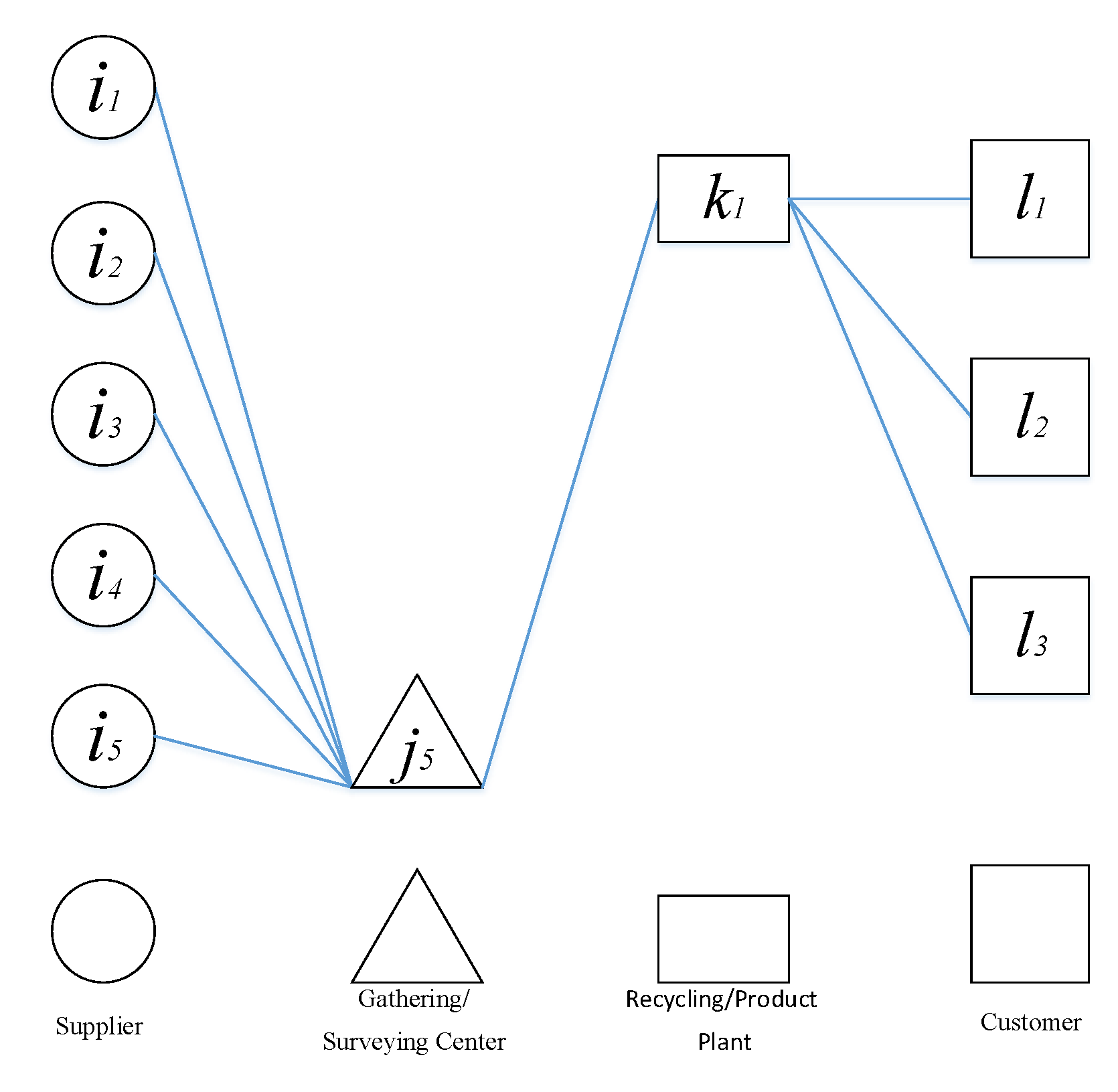
As expected, due to the high cost of constructing facilities in the steel industry, one center (center number 5) of the five candidates was selected, and one factory (factory number 1) of the three nominated recycling/production plants for construction is calculated, and it provides an excellent answer to the case study. In this way, the schematic of the reverse SC model is changed after the solution, as shown in Figure 6.

Besides, the values of the parameters of the NSGA-II algorithm are described in

Table 15. The values of the algorithm NSGA-II operators for the case study.

	MaxIt	nPop	Pc	Pm
NSGA-II	100	100	0.6	0.3

in the main model.

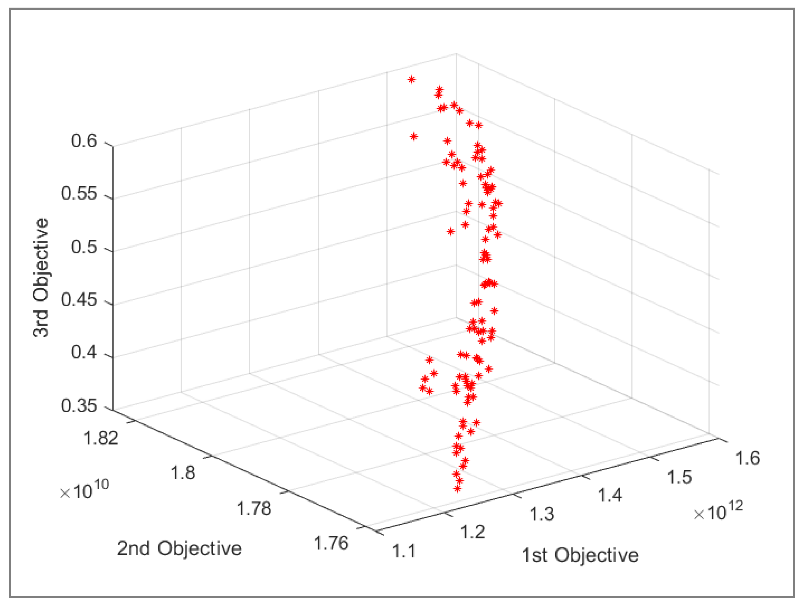
For any Pareto optimal solution, the optimal values of decision variables are obtained(see Figure 7). For instance, the magnitudes of some decision variables for the first Pareto solution in Table 14 are represented in

Table 16. A sample of optimal decision variables for the first Pareto solution of Table 14.

Variable	Value	Variable	Value
QSR1,5,1,1,1	2.4605	QSR1,5,2,1,1	7.9593
QSR2,5,1,1,1	2.9064	QSR2,5,2,1,1	7.7476
QSR3,5,1,1,1	6.1607	QSR3,5,2,1,1	11.3636
QSR4,5,1,1,1	8.0460	QSR4,5,2,1,1	7.8387
QSR5,5,1,1,1	4.5488	QSR5,5,2,1,1	6.7933

. According to this table, under the first scenario, a magnitude of 2.4605 of the first product type should be transported from the first supplier to the fifth gathering center. Other values can be interpreted similarly. For each Pareto optimal solution, a similar set of optimal decision variables is obtained.

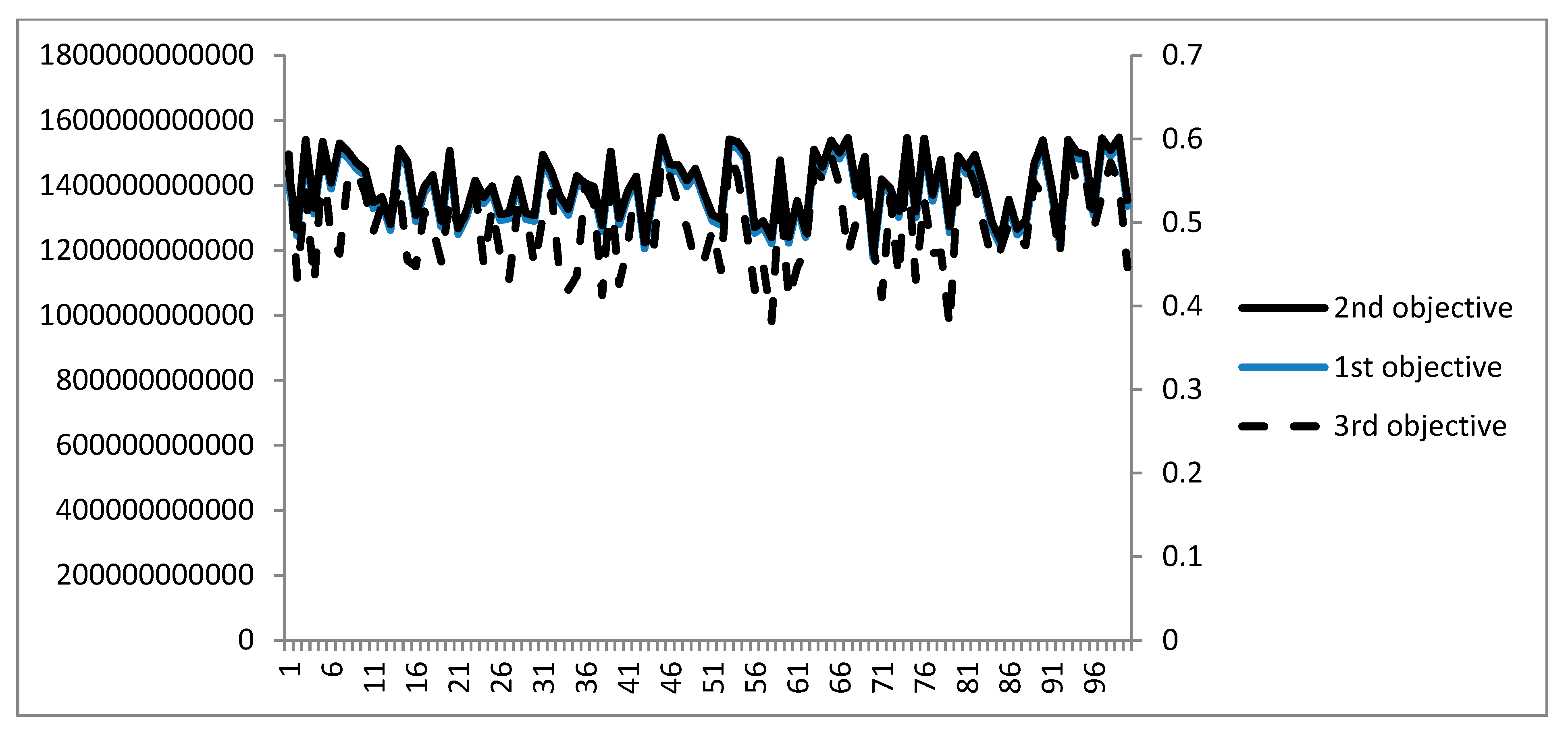
To assure the convergence of the proposed algorithm, with its tuned parameters, the above problem is repetitively solved 100 times. Figure 8 illustrates the obtained results of the solutions for different objectives. According to this figure, it is clear that the algorithm-proposed solution in all of the objectives represents a controllable variance, and it can be considered as the proposed algorithm reliability. No outlier solutions can be detected in repetitions.

3.8. Sensitivity Analysis

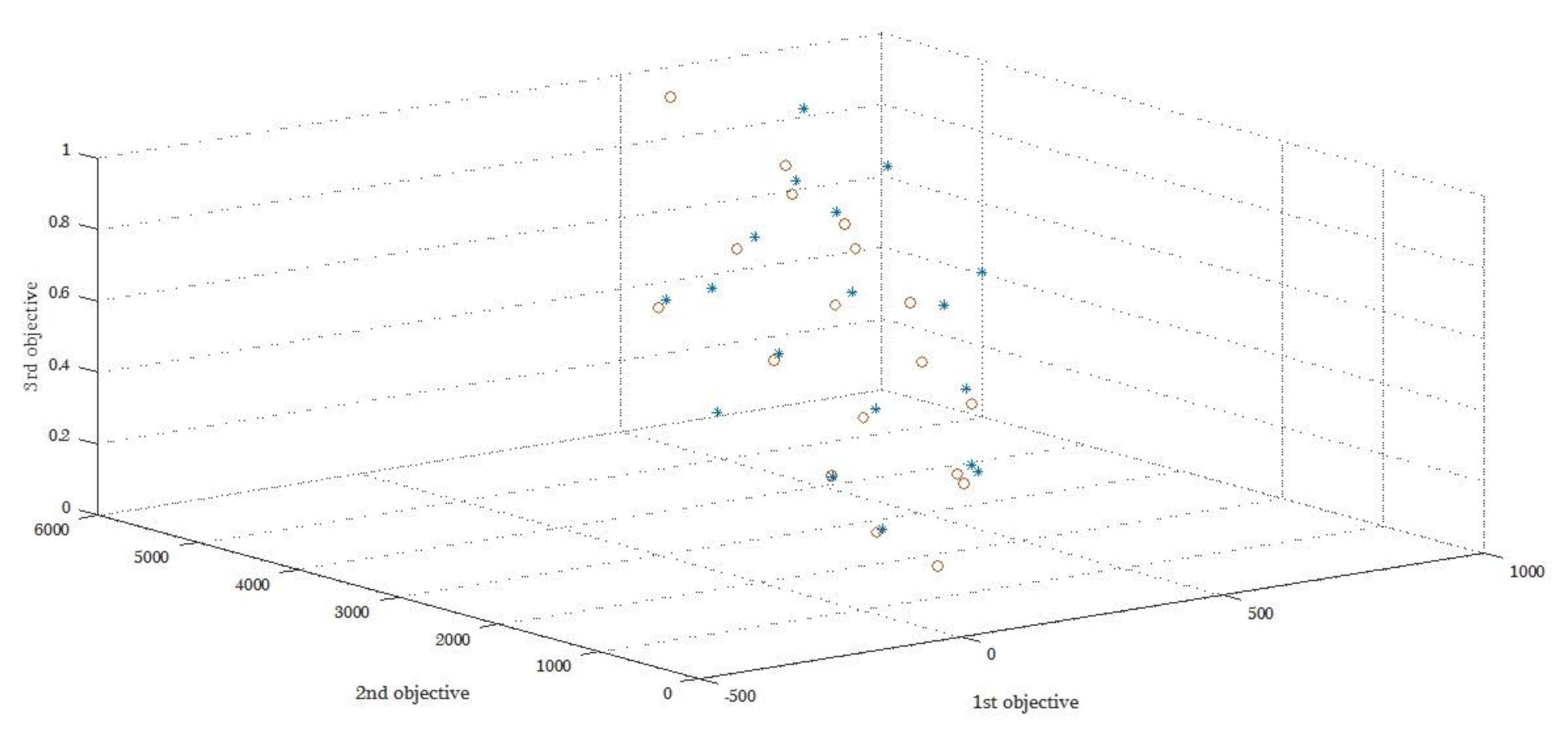
To investigate how the values of the objective functions varied, sensitivity analysis should be performed on some of the parameters. Regarding the multiplicity of the model, two types of analysis are performed. The first type is the change in Pareto’s values relative to the change in one of the parameters. In the present study, this type of analysis—as compared to the change in the demand parameter in the initial model, which decreased by 10%—and the results of this sensitivity analysis are shown in

Table 17. Changes in Pareto points for the initial model induced by changing the value of demand.

No.	Before Changing the Demand Parameter			After Changing the Demand Parameter
	Amount of 1st O.F.	Amount of 2nd O.F.	Amount of 3rd. O.F.	Amount of 1st O.F.	Amount of 2nd O.F.	Amount of 3rd. O.F.
1	−128.17	2271.64	0.8	−170.57	2117.32	0.8
2	−247.05	1135.82	0.6	−92.47	801.17	0.41
3	−92.47	801.17	0.41	42.57	1058.66	0.2
4	67.78	1135.82	0.2	49.15	2117.32	0.6
5	87.77	2271.64	0.6	158.82	1058.66	0.08

and Figure 9.

As demonstrated, with the decrease in the average demand, the value of the objective function decreased. By virtue of shipping costs, other items are reduced by decreasing demand. In Figure 4, the stars represent the Pareto before the change, and the circles represent the Pareto after the change.

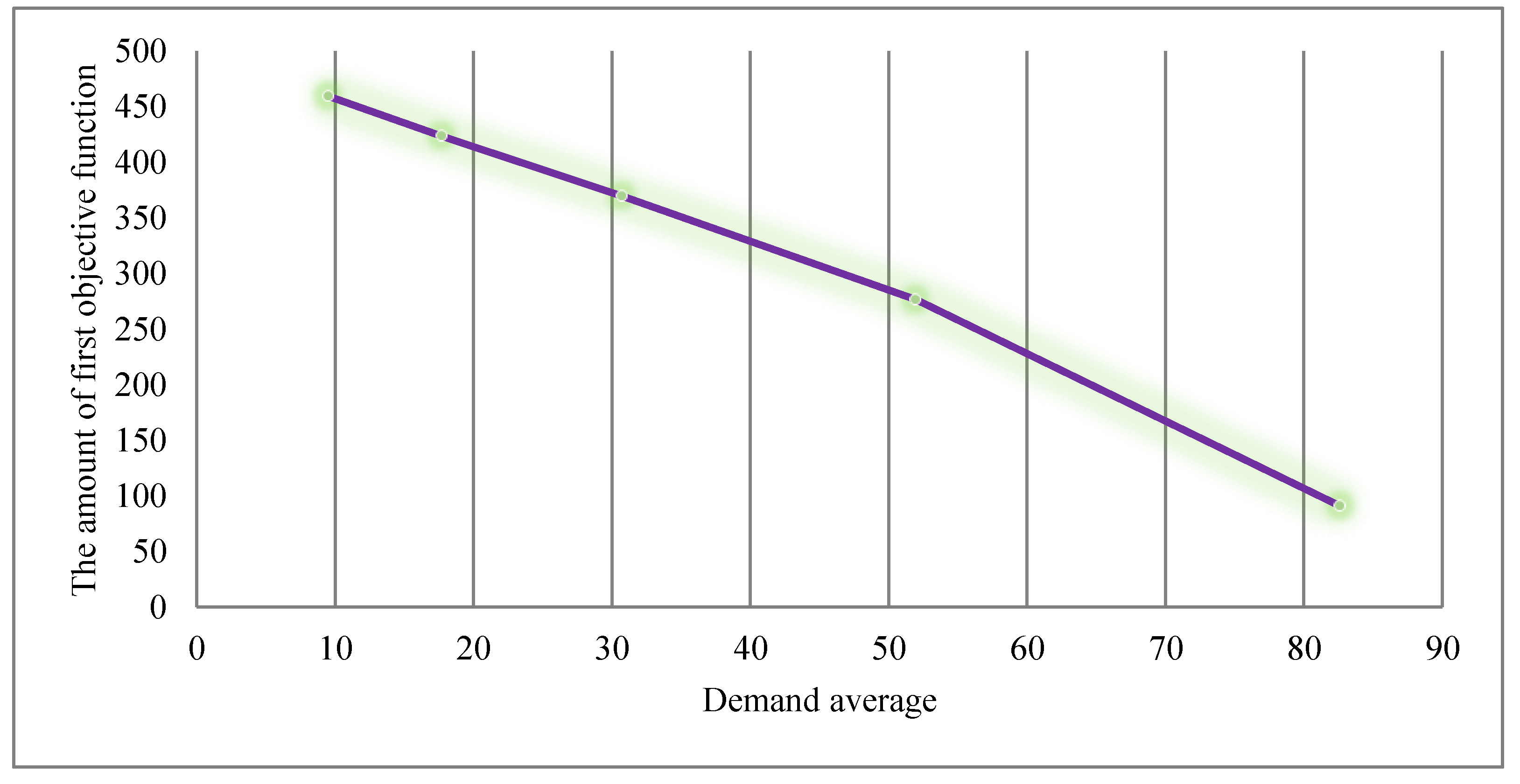
The second type of sensitivity analysis is employed for one Pareto point (here, for the tenth Pareto point), which is done for the demand parameter. The variability of the value of the objective function concerning demand in the initial model is shown in

Table 18. Changes to the first objective function for the initial model induced by changing the amount of demand.

Item	The Amount of Demand Average	The Amount of First Objective Function
1	9.57	459.08
2	17.76	423.237
3	30.765	369.45
4	51.994	276.155
5	82.643	90.683

and Figure 10.

In Table 18, by assuming that the second and third objective functions are fixed, and that only the changes in the first objective function have been investigated, it is seen that with increasing average demand, the first objective function is reduced. In fact, with increasing demand, the amount of cost is higher than the amount of income.

4. Discussion and Conclusions

In the present study, the model was defined as multi-objective functions based on the conditions of the uncertainty of demand and five scenarios; the model was solved by an augmented epsilon constraint method and the NSGA-II algorithm, and finally analyzed. This proposed model is based upon the work of Feito Cespon et al. 2017 [22] by using a different objective function and case study and different solving approaches to compare the results. Because the number of levels and actual data of the model would be Np-hard by solving the GAMS, and it would not be able to achieve the optimal response, model validation and sensitivity analysis were done on a smaller scale. The results of the comparative indices showed that solving the model with the NSGA-II algorithm yielded acceptable results, and the main model was solved accordingly. Additionally, the optimal levels of the NSGA-II algorithm parameters were adjusted in the original model, based on the Taguchi design of experiments method. In analyzing the results, as expected, in the locating facility, one gathering center was selected from five candidates, and one recycling plant was selected from three candidate plants. The number of objective functions in different Pareto points has been obtained with a suitable and acceptable dispersion criterion. The model showed that it could be integrated into optimizing the objectives, determining the number and location of necessary facilities and planning the transportation between different levels of the steel industry. Some of the assumptions implied in the current study can be adjusted in future studies. First, there are some general assumptions including the uncertainty of demand parameter, the determinedness of costs, the number and capacity of transportation modes and the number of supply chain levels. These assumptions can be generalized straightforwardly, by considering the uncertainty of other parameters and extending the model into more levels. Additionally, in the current paper, it is assumed that the number of suppliers, customers, gathering centers and recycling plants are determined. However, in some cases, the problem can be formulated to select different markets, suppliers, and gathering and recycling centers in a broader scope. These extensions will not change the structure of the proposed method drastically. However, altering some assumptions requires fundamental changes in the proposed model. Among these assumptions, reference to transshipment among levels (ignoring the sixth assumption) and limiting the capacity of gathering centers and recycling plants can be made. Further research can be done on the above-mentioned problems by changing the current model’s assumptions.