Abstract
A new compound non-symmetric distribution for modeling arbitrary fading-shadowing wireless channels is introduced and studied here. This distribution has some advantages in front of other well-known non-symmetric fading distributions such as the Rayleigh–lognormal distribution and the K distribution especially in the tails. We give closed-form expressions for the average BER of DPSK and MSK when the new distribution is used. Applications to compare how the new distribution works in comparisons with the Rayleigh–lognormal, K distributions and others recently proposed in the literature of fading channel are also provided.
1. Introduction
Systems of mobile communications rising to the challenge of the 5G framework demand high data rates at a low latency [1,2]. This new communication paradigm includes device-to-device, vehicular communications, machine-to-machine as well as traditional communications provided by ground base stations. Such mobile systems face several challenges that degrade signal strength. Among them, fading is the more relevant and it has been widely researched in past decades. Generally speaking, fading refers to the interference of multiple scattered radio paths (radio waves) between the base station (ground base station or another emitter) and the vicinity of the mobile receptor. As mentioned above, this definition is now enhanced to account for the new device-to-device communication systems, although in this case, new constraints hold (because the channels are symmetric from left-to-right and right-to-left, they become indistinguishable). Due to signal fading, the received signal at the device exhibits fast signal level fluctuations which are normally Rayleigh distributed. The direct consequence of fading is the complete loss of signal (or a large decrease of the received power).
In a simplified manner, although the emitter emits a unique wave (a ray), the received radio signal is composed of the superposition of the set of many waves (randomly distributed) that come from the multiple dispersion experimented by the original wave. Each of these scattered waves may have a different amplitude and phase. Therefore, what was originally a single path channel is now transformed into a multichannel one. This complex channel can be modeled as a truly physical communication channel characterized by its bandwidth and gain (see the seminal work by Beckmann [3] for a complete description of modeling of multi-path channels). For the common case of a mobile radio channel characterized by a constant gain and a linear phase response across the bandwidth greater than the bandwidth of the transmitted signal (common real situation), the signal at the terminal will show what is known as flat fading, which is the most common and consequently the most researched [4]. Due to fading, the strength of the received signal will show oscillations (even very fast oscillations) in time caused by the multi-path effects.
Figure 1 shows a simplified fading model for a stationary source (emitter at ground base station) and a mobile receptor (vehicle) where several signal components are involved (see a complete description of fading modeling in [4,5,6,7]). A similar figure can be used to account for device-to-device 5G mobile terminals. First, for the case of clear line of sight between stationary source (emitter) and moving receptor, no scattering mechanism would be involved, although Doppler effects would be taken into account. Moreover, the multi-path component, also known as the diffuse component (phase-incoherent wave) is caused by the several (random) reflections (scattering processes) of the signal with scattered elements such as buildings and mountains or other elements (vehicles, people...). This component exhibits little directivity and its magnitude is usually assumed to be Rayleigh distributed, while its phase is distributed uniformly. The other component shown in this figure is the specular component: a phase-coherent ground-reflected wave caused by close points to where the receptor (moving vehicle in this case) is dynamically located [8]. It is responsible for deep fades (probable critical loss of signal power), with its amplitude comparable to the one for the direct component, although its phase is opposite [9].
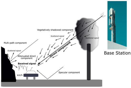
Figure 1.
Illustration of fading components.
In the same figure, the case of blocked line of sight between the stationary source (emitter) and the mobile receptor is also shown. In this case, the diffuse component shows a similar behavior than before (and it can be also modeled by a Rayleigh distribution based on the assumption of a sufficiently large number of received waves at mobile terminal), but a new component appears: the shadowed direct component. This component is due to the scattering of the signal by branches, leaves, and limbs of nearby trees and surrounded vegetation in general. This scattering mechanism is indeed very complex to model. As a consequence of that, the signal is attenuated. The amount of signal attenuation depends on the length of the path of the signal through the scattered element (tree, bushes, etc.). The fading related to this process is known as fading-shadowing and it may be suitably modeled by the Rayleigh–lognormal distribution (RLN in advance) [10] which has a difficult integral form. It can be better modeled by the well-known K distribution [11]. The K distribution is indeed a Rayleigh distribution with a gamma distribution, and it has a simpler form than the RLN.
In this paper, we focus on the fast fading-shadowing mechanisms. Furthermore, as our work also includes the Rayleigh as a general case, it also may be applied to dealing with the diffuse component.
From above, it is clear that a precise characterization of the received radio signal is not possible and, as the nature of the wireless channel is random, statistical characterization through suitable probability density distributions is required [12]. For a given probability distribution aiming to efficiently model fading effects, it is desirable for it to be expressed by means of simple mathematical formulas and it shall embed the Rayleigh distribution as a particular case. This latter condition comes from the fact that Rayleigh modeling of scattered signal resembles as the natural approach for multi-path fading modeling and it provides a direct physical explanation for parameters involved (signal phase and signal power). For such fading distributions, the estimation of parameters is easy, and metrics commonly used to characterize fading effects (LCR, level crossing-rate, AFD, average fade duration, BER, average bit error rate, DPSK, differential phase-shift keying or MSK, minimum shift keying) are also easily obtained (see [13,14,15]), for a thorough explanation of these well-known quality indices for measuring channel capacity and reliability).
Since the work provided by Beckmann [3] to describe the statistical fading envelope (summation of all scattered waves) of the received signal, a plethora of distributions in this setting has been proposed. As seen from the revision of related works, such statistical models span from classical distributions such as the Rayleigh (see a review of fading channels modeled by using the Rayleigh distribution in [16]) to new ones, such as the Nakagami distribution [17,18], also including joint distributions such as the Rayleigh–lognormal [19] or other distributions [20,21].
In [22], a new two-parameter fading distribution, the SR (Slashed Rayleigh), was proposed. This distribution naturally includes the Rayleigh distribution as a particular case when one of its two parameters is reasonably large, thus facilitating the physical modeling of multi-path signal propagation by suitable phasors (complex signal representation). The SR fading distribution is competitive with the Rayleigh–lognormal distribution and the K distribution.
In this work, we present the two-parameter compound distribution RBS (Rayleigh Birnbaum Saunders) for multi-path fading modeling. This distribution has some advantages in front of the Rayleigh–lognormal distribution and the K distribution, especially in the tails. We give closed-form expressions for the average BER of DPSK and MSK when the new distribution is used. We complete the description of the RBS distribution by explaining how to simulate it by means of Monte Carlo analysis, and what is mandatory for a fading distribution, by simulating it as a summation of phasors also including Doppler effects (that is, a physical description) by suitable embedding of the RBS distribution into the well-known Clarke’s model [4] for flat fading.
We remark that although fading effects are more noticeable for mobile communications (i.e., people in urban areas quiet or moving), fading is more remarkable for land mobile vehicles because, as they are travelling faster, most received signal is due to multi-path components instead of the direct component. However, for a stationary receiver (for instance, working with a tablet), if the surrounding objects are moving faster than the mobile terminal, Doppler shift on multi-path components may significantly influence the transmitted signal quality. Therefore, the models discussed in this work are also valid for both situations: stationary receptor and moving receptor.
The outline of this paper is as follows. A catalog of the distribution functions usually used in this setting is provided in Section 2. This Section also includes the Birnbaum Saunders distribution and its more important properties. The proposed new fading model is provided in Section 3. Section 4 is concerned with most important measures of interest in the setting of a fading channel, such as the channel capacity, the AF and the BER for DPSK and MSK when the distribution introduced here is used for fading channel modeling. Comparisons with other distributions usually used in the setting of fading channel are given in Section 5. Simulation results are provided in Section 6, and conclusions are in the last Section.
2. Background
Rayleigh fading is a reasonable model when there are many objects in the environment that scatter the radio signal before it arrives at the receiver. The central limit theorem holds that if there is sufficient scatter, the channel impulse response will be well modeled as a Gaussian process irrespective of the distribution of the individual components. If there is no dominant component to the scatter, then such a process will have zero mean and phase uniformly distributed between 0 and radians. The envelope of the channel response will therefore be Rayleigh distributed, with probability density function (pdf)
where is the expected value of being . In this case we will write .
As Tse ([23] p. 49) has pointed out, [sic] the model based on the Rayleigh fading, is quite reasonable for scattering mechanisms where there are many small reflectors, but is adopted primarily for its simplicity in typical cellular situations with a relatively small number of reflectors. Due to the fact that several alternatives to Rayleigh fading have been proposed in the literature, some of them will be shown next. The Rayleigh–lognormal distribution (RLN) with pdf is given by [10,24]
The Rayleigh-Gamma distribution (K distribution) [11] obtained by compounding a Rayleigh distribution with a gamma distribution is similar to the RLN distribution but it has a simpler form and its pdf admits a closed form but, due to the Bessel function, the estimates of the parameters are not direct. Its pdf is given by,
with being the usual gamma function and
denoting the modified Bessel function of the second kind of order and argument z.
The Rayleigh-inverse Gaussian (RIG) distribution has pdf given by
with and .
The generalized Rayleigh distribution (GR in advance), built as a mixture of the Rayleigh distribution with a geometric one, proposed in [25], has pdf given by
with and .
Finally, we consider the Slash-Rayleigh distribution (SR), recently proposed by [22] which has the pdf given by
where , and represents the Kummer confluent hypergeometric function.
It is interesting to note that this special function appears in most of the statistical packages available the market, such as R, MATLAB and Mathematica, which has been widely used in this work (see [26]). Other alternatives based on the lognormal distribution apart of the RLN distribution, which will not be used here, are the Rayleigh-inverse Gaussian distribution (RIG) [27] with the same restriction as the above distribution and the generalization of the Rayleigh distribution proposed recently by [25], which overcomes many of the disadvantages of the mentioned distributions.
The Birnbaum Saunders Distribution
From the pioneering work about the Birnbaum Saunders distribution proposed by [28,29] a lot of works about this distribution have been proposed in the statistical and applied statistical literature. For a comprehensive reading of this distribution see [30]. The distribution was introduced in the context of fatigue life problems although today it is applied in very different contexts. A continuous random variable X follows a Birnbaum Saunders distribution with parameters and if its pdf is given by
where represents the pdf of the standard normal distribution. The raw k-moment of the distribution is given by
from which we get the mean and variance of (2) given by
respectively, while the cumulative distribution function, , is given by
where is the survival function of the standard normal distribution. The moment generating function is given by
where .
3. The Proposed Fading Channel Model
The compound distribution proposed here is obtained by compounding the Rayleigh distribution given in (1) with the Birnbaum Saunders distribution provided in (2) and has pdf (see details in the Appendix A) given by
where . In what follows, when a random variable R follows this distribution it will be written as to denote that the distribution is obtained by compounding the classical Rayleigh distribution with the Birnbaum Saunders distribution.
The new distribution is unimodal with a modal value being the solution of the equation
Some graphics of the pdf of the distribution are shown in Figure 2 where the dependency of the scale parameter and the shape parameters (the fading) can be appreciated.
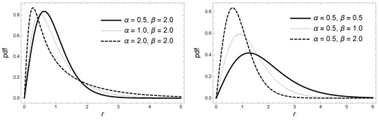
Figure 2.
Probability density function of the distribution for different parameter values.
Additional Features
The survival function (the probability that the envelope of the received signal does not exceed a specified value of r), of is given by (see the Appendix A)
which can be used to get the hazard function of the random variable , given by
Some plots of the hazard rate function in (6) are displayed in Figure 3 for special cases of parameters.
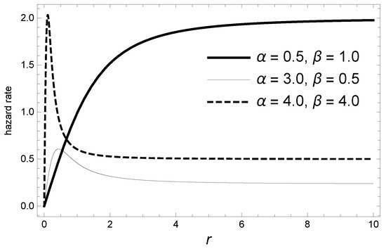
Figure 3.
Illustration of the hazard rate function of distribution for a set of different parameter values.
Let . Then, for and , it follows that k-th moment of the proposed distribution is given by
which can be obtained by compounding taking into account that the kth moment of the Rayleigh distribution are given by
Therefore, by using (7) we get the mean and the second raw moment of the distribution, which are given by
respectively. Now, the variance can be obtained directly from (8) and (9). Maximum likelihood estimation can be obtained by maximizing the log-likelihood function, which is proportional to
where n is the size of the sample . Thus, the estimators of the parameters can be obtained by solving the equations,
where
are the partial derivatives of with respect to and , respectively.
Furthermore, since the RBS distribution can be represented as a mixture (compound) of the Rayleigh distribution and the Birnbaum Saunders distribution, this representation of the distribution also facilitates parameter estimation via the Expectation Maximization (EM) algorithm.
4. The RBS Channel Phasor
In this section, we demonstrate that the RBS distribution can be obtained as an exact sum of mutually independent Gaussian stochastic processes, as is required for the simulation of the fading channel, i.e., to estimate the signal envelope.
Rayleigh fading envelopes can be generated from the zero-mean complex Gaussian random variables. Other fading distributions (see for instance [31] for the Nakagami-m case) and the generalized Rayleigh distribution in [25] can also be obtained in a similar manner after some mathematical considerations. Following those works, it is necessary to prove that the phase of a given propagating signal is uniformly distributed in the interval and that the amplitude follows a RBS distribution.
Following (Beckmann [3] p. 118),
where , the terms X (the in-phase phasor) and Y (quadrature phasor) are independent uniformly distributed phasors (UDP) and the are all distributed identically. When n is large and we assume that is not correlated with the , both X and Y will be distributed normally with mean 0 and variance . [32], see page 69, has pointed out that under some conditions this is also true for small n. Let now . Then, the joint distribution of X and Y is
Then, expressing (11) in polar coordinates results
Thus, it is simple to see that the phase distribution is uniform, i.e., . On the other hand, the (unconditional) amplitude distribution is given by (5).
Some Measures of Interest in the Setting of Fading Channel
Since the RBS distribution studied here can be obtained easily as a mixture of the Rayleigh distribution and the Birnbaum Saunders distribution this strongly facilitates the calculus of relevant measures of interest (quality indices) within the framework of fading channel: the amount of fading (this is known in the literature also as strength of intensity fluctuations), AF and the BER for DPSK and MSK when the distribution introduced here are applied to modeling a mobile communication channel.
For a SISO (single-input-single-output) system, the amount of fading, a unified measure for the severity of fading (see for instance [33]), is based on the moments of the fading distribution and is given by . For the distribution studied here is given by
which does not depend on and is larger than 1, the value of AF for the Rayleigh, , distribution. Observe that when we have .
From [11], it is known that for the standard Rayleigh distribution, , the BER for DPSK and MSK are given by
respectively.
Now, we can obtain, by compounding, and for the special case in which the corresponding average BER of DPSK and MSK for the RBS distribution. They are given in the following result.
Proposition 1.
Suppose that , then the average BER of DPSK and MSK for the RBS distribution are given by
respectively. Here , where is the transmitted energy per bit and is the noise power spectral density.
Proof.
Using the negative binomial series
and using the composite rule we get
from which is obtained now by using (3). is calculated in a similar manner. □
The average channel capacity for fading channel is a good metric as it gives an estimation of the information rate that the channel can support with small probability of error. Channel capacity, C, (see for instance [34,35], among others) is defined as
where B is the received signal bandwidth. Following [34] it is known that the Shannon capacity of the Rayleigh fading channel is given by
where , , S the average transmit power receiving bandwidth B and the mean channel gain . Thus, the unconditional channel capacity can be obtained numerically by computing the following integral
Another way of computing the latter integral is to use the series representation of the exponential integral function (see [36,37]) which establishes that
where is the Euler’s constant.
5. Some Measures for Comparing
In Figure 4, the average BERs are plotted for DPSK and MSK for RLN, K and SR distributions for the three sets of parameter values given in Table 1. The BER for RLN and K distributions were numerically obtained for DPSK and MSK using the same values of parameters for the K distribution taken by [33] in three settings. Setting A is for value, Setting B is for value and Setting C is for value. For all the cases , as indicated in the same table. The corresponding values of the parameters for the RLN and RBS distributions were obtained by equating the population moments to the moments of the K distribution obtained from the above a and b values. Recall that the population moments of the K and RLN distributions are given by and , , respectively. Moments of the RIG, GR and SR distributions can be found in [22,25,27], respectively. First and second moments of the RBS distribution were taken from (3). The estimated parameter values of the RLN distribution, and , obtained here are different from the ones obtained by [33] since they used the approximation provided in [11].
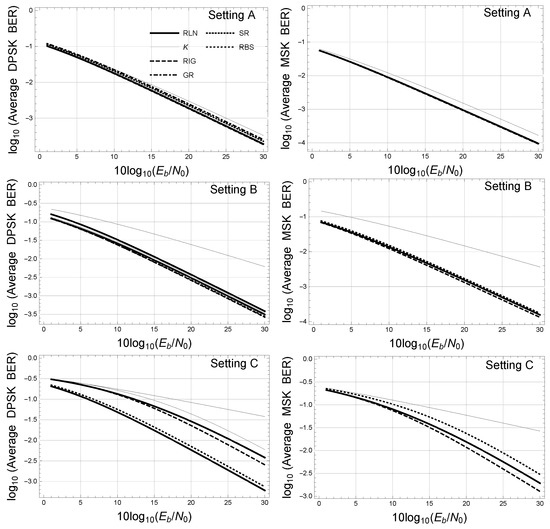
Figure 4.
Average BERs of DPSK and MSK for RLN, K, RIG, SR and RBS distributions assuming values for the parameters given in different settings provided in Table 1.

Table 1.
Values of the parameters for RLN, K and RBS distributions.
In view of the graphs, the utility of the RBS distribution for the prediction of BER in multi-path dispersion fades can be inferred. We must also influence the good fit, compared to the distribution K, between the proposed distribution and the RLN distribution. The third scenario is conclusive in this case. Recall that the RLN distribution is commonly used in all DPSK and MSK modulation schemes. It is also worth noting that for the RLN distribution, there is no closed-form expression for the average BER, which must be calculated by means of numerical integration methods (generally, the Gauss–Hermite method). An exact but complicated formula for estimating the BER in the DPSK case when the RLN distribution is used is reported in [38].
On the other hand, comparing the analytical expressions of the proposed distribution and the K distribution, both include special functions in their formulation—the incomplete gamma function and the modified Bessel function, respectively. Then, from this point of view both are similar and therefore an alternative to it, which has been used as a substitute for the RLN distribution.
From the above, it is clear that the proposed distribution can be applied to deal with the bleached shading aspects of the wireless channels.
Figure 5 shows the pdf of the different distributions used for parameters given in Settings A and B. It seems that all distributions provide similar tails.
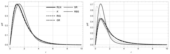
Figure 5.
Graphics of the pdf of the different distributions for parameters given in Settings A (left) and B (right).
Comparison with the RL, K and RIG Distributions
It is well known that we can study the distance or relative information between two probability distributions by using the Kullback–Leibler divergence measure (see [39], among others) which is defined as follows: Let f and g be probability densities on such that f is absolutely continuous with respect to g (that is, implies ), then the relative information or Kullback–Leibler divergence, of f with respect to g is
with the convention that . When f is not absolutely continuous with respect to g we define . One of the disadvantages of (15) is that the Kullback–Leibler divergence is not symmetric and therefore is not a genuine distance metric. To surpass that, the Jensen–Shanon divergence (see for instance, [40]) given by
where , and the integrated squared error, ISE, [41] given by
will be used.
Table 2 includes the Jensen–Shannon divergence for all the distributions considered here. We can see that the RBS distribution provides a distance similar to the ones provided with the rest of the distribution. Here the RL distribution was taken as the reference distribution.
Table 2.
JSD and ISE measures for K and SR distributions (compared to the RLN distribution).
6. Simulating the Proposed Distribution
To model a fading process, simulation of a random variable is required following the distribution. Additionally, this task must be done at low computational cost (because not a single variable, but thousands of them, are needed). In the literature, there are many methods to do that. In this work, we follow the same method used in [25], applying the standard inverse transform method because this method is simple and easy to implement. In Algorithm 1 a simplified version of the inverse transform method is summarized. The cdf (cumulative density function) corresponds to , i.e., expression (8). Indeed to , which is obtained at low computational cost and can be even pre-calculated for a set of and parameters to speed up the simulation.
The simulation of the variable was coded in MATLAB and executed on an i7-7700HQ CPU @ 2.80 GHz (16 GB RAM), taking around seconds to generate (one million) random variates. The program is efficiently coded in a matrixial way (it does not use loops). The computational cost is indeed low, hence, well suited to fading channel modeling.
By Monte Carlo simulations, two large datasets were obtained ( samples) and compared with the analytical RBS pdfs. In Figure 6, the analytical pdf for the RBS distribution and the ones from simulated data, which clearly show a good fit for both datasets, can be seen. As expected, the error for the variance is larger than for the case of the mean but certainly low for both measures for the two cases shown. See also the analyticle and simulated values for the mean and variance in Table 3.
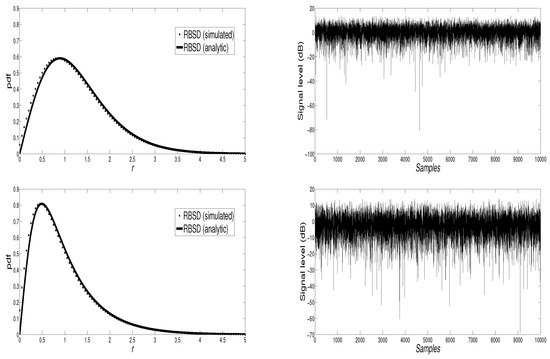
Figure 6.
Comparison of the analytic RBS(, ) magnitude pdf and the Monte Carlo simulated dataset (top). Comparison of the analytic RBS (, ) magnitude pdf and the Monte Carlo simulated dataset (bottom). Simulated samples (1,000,000) for both cases are also represented (right column).
Table 3.
Mean and variance values for the analytic RBS distribution and those estimated from the simulated samples for two sets of parameters.
However, to properly simulate the fading effects for a communication channel, the simulation must be done in terms of phasors (see Section 4) and coupled to physical variables (signal carrier frequency, signal sampling, speed of receiver and Doppler effects) related to the channel. These issues are discussed in the next section.
| Algorithm 1: Simulating the RBS distribution. | |
| Input: | |
| Alpha: parameter () | |
| Beta: parameter () | |
| A: range of data (Amplitude ) | |
| NumberSamples: number of samples (NumberSamples ) | |
| Output: | |
| S: set of data | |
| Begin: | |
| r ← CDF(Alpha, Beta) (0 → A) | ⊳CDF to a column vector for do |
| end | |
| ⊳Get a uniform random | |
| number | |
| End | |
The RBS Distribution for Modeling Fading Effects
In this section, we proceed as in [22]—which is also based on the classical well-known Clarke’s model [4], but we present the model for the sake of completeness of this work. First, we reformulate the phasors obtained in Section 4 as follows:
as explained, for instance, by [4] as follows,
where is the amplitude of the transmitted signal (). The phase is replaced by the term . The phase is the random phase (uniformly distributed in the interval ), accounts for the Doppler shift, where v is the receptor velocity, represents the wave number, is the wavelength and is the maximum Doppler shift (in units of radians per second). The angle of arrival of the transmitted wave is , also distributed in , and N is the number of harmonic waves, which, if large enough (as expected in the real case), ensures that both and are Gaussian processes. From that, the RBS signal envelope is given by , and The amplitude of the envelope is then suitably fitted to the RBS amplitude of the transmitted signal to assure that RBS.
By using this model, a Monte Carlo simulation (using 15 scattered random phasors and 20,000 samples) was performed to obtain the dataset (random samples) and from that, the pdf is ensembled to compare it with the analytic RBS pdf. This comparison is plotted in Figure 7 (left column) for two sets of RBS distributions ( and, ). As can be seen, a reasonably good fit between the analytic and the physical models is obtained. On the right column of the same figure, a set of simulated samples for both cases is shown. As expected, these samples are mostly near the mean value provided by the parameter setting. Deep fading effects ( dB) are present. Hence, the RBS distribution naturally accounts for the presence of large fading values related to minimal power received at the terminal).
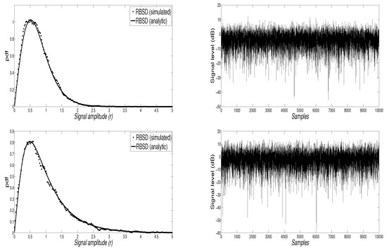
Figure 7.
Samples simulated by using phasors of the RBS distribution ( = 0.5, ) (top, left) and a set of simulated samples (top, right). Samples simulated by using phasors of the RBS distribution ( = 1, ) (bottom, left) and a set of simulated samples (bottom, right). For both cases, the analytic RBS distribution is also shown, for the sake of comparison.
Table 4 contains the analytical means and variances compared with those estimated from the Monte Carlo data. The relative errors (percentual values) for both measures and for both datasets are acceptable (less than 5% and lower that 1% for the variance for the set and ), but noticeably larger than when the data were generated directly from the respective cdfs. This is due to the complexity of this simulation, which accounts for physical effects (wave scattering).
Table 4.
Means and variances for the analytic distribution and, the values estimated using phasors for two-parameter sets.
Figure 8 illustrates SR, the RLN, and the proposed RBS distribution. The parameters used in all cases are those providing similar mean (emitted power) and standard deviation values, and are plotted spaced 0.1 wavelength apart for the 0 dB mean value. As can be seen, the RBS distribution shows a behavior similar to the Rayleigh and to the SR distributions but capturing deep fading effects. Additionally, the RBS distribution seems more suited to modern communication systems, and more robust to fading effects.
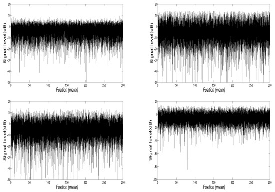
Figure 8.
Simulated samples (using phasors) of the Rayleigh fading distribution (top left), the SR fading distribution (top right), the RLN fading distribution (bottom left) and, the proposed RBS fading distribution. The parameters used in all cases are those providing similar mean and standard deviation values, and are represented spaced 0.1 wavelength apart for the 0 dB mean value.
Finally, a simulation of the physical channel is performed to illustrate that the proposed RBS distribution efficiently models fading effects. In what follows, we also proceed as in [22].
Algorithm 2 details the pseudo-code used for the channel simulation (Clarke’s model). To generate a realistic fading spectrum (that is, to generate time-correlated fading waveforms), a common baseband Doppler filter was also included in the simulations.
Figure 9 shows the simulated fading signal for the RBS(, ) distribution, corresponding to a signal with a power mean value of 1. Fifteen Rayleigh processes (rays) and 20,000 samples were simulated to obtain the envelope. In this case, the envelope includes deep fading levels (relative to the low power used) due to fast fading in long-distance HF (High frequency) propagation ([31]). The results discussed above were for two vehicles at velocities 50 km/h and 120 km/h, respectively. As expected, the Doppler effect is more noticeable as the vehicle velocity increases.
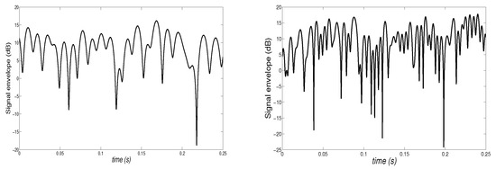
Figure 9.
Fading signal for the RBS distribution (, ); carrier frequency = 1 GHz and speed = 50 Km/h (left) and speed = 120 km/h (right).
The physical meaning of the parameters of the RBS distribution has not been discussed in this paper. However, from expression (8), and also from Algorithm 2, it seems clear that they depend on the average signal power strength of the emitter. However, a deeper analysis must be done.
To get all data shown in this paper, a fading channel program has been developed (coded in MATLAB and using a friendly graphic interface). The prototype implements the Clarke’s model, and it also includes standard signal processing routines (filters) and all the metrics to characterize the channel as well as the other standard fading distributions (i.e., Rayleigh, SR and RLN).
| Algorithm 2: Fading simulation. | |
| Input: | |
| Alpha: parameter () | |
| Beta: parameter () | |
| Rays: number of emitted signals (Rays ) | |
| Ref: number of reflections (Ref ) | |
| Speed: average speed of vehicle (Speed ) | |
| Freq: carrier frequency (Freq ) | |
| TimeF: simulation time (TimeF ) | |
| TimeS: sampling time (TimeS ) | |
| Output: | |
| r: signal envelope | |
| Begin: | |
| A ← getPower(Alpha, Beta) | ⊳Get average signal strength and variance |
| Phi ← rand(Rays, Ref) | ⊳Uniformly distributed phase |
| Psi ← rand(Rays, Ref) | ⊳Uniformly distributed arriving signal |
| D ← Freq· 3.3e-03 | ⊳Maximum Doppler frequency shift |
| w | ⊳Consider Doppler effects |
| t ← 0: TimeS: TimeF | ⊳Time span |
| X ← 0 | |
| Y ← 0 | |
| Df | ⊳Obtain Doppler phase shift |
| ⊳In-phase component | |
| ⊳Quadrature component | |
| end for | |
| end for | |
| ⊳Calculate the signal envelope | |
| End | |
7. Final Comments
In this work, we proposed a new distribution, the two-parameter Rayleigh Birnbaum Saunders Distribution, which shows some benefits in comparison with the Rayleigh–lognormal distribution, the SR distribution and, the K distribution. The Rayleigh distribution is included as a particular case when one of its parameters is large enough. The estimation of the parameters of the proposed distribution has been also taken into account. The new distribution we propose shows clear advantages when compared to the Rayleigh–lognormal distribution within the framework of fading signal modeling. Signal envelope has been obtained through two different methods: from the analytic pdf and from physical simulation of the communication channel by means of phasors using Clarke’s model. The common metrics for estimating the quality of the received signal (the bit error rate (BER) for DPSK and MSK modulations) have also been derived in closed form for the new fading distribution. Future work will focus on providing a physical meaning for the parameters of the RBS distribution, and , although some preliminary clues were already given above.
Data Availability
Reproducibility of data used to support the findings of this work can be done through the mathematical formulas and algorithm explanations included within the article. Additionally, codes used are available from the corresponding author upon request. These data include Mathematica and MATLAB codes, therefore users should have their corresponding software licenses.
Author Contributions
The methodological part of this work constitutes a contribution of the first author, while all applications are the work of the second. Both co-authors contributed to the editing, discussion and review of this manuscript. All authors have read and agreed to the published version of the manuscript.
Funding
EGD was partially funded by grant ECO2017-85577-P (Ministerio de Economía, Industria y Competitividad. Agencia Estatal de Investigación)).
Conflicts of Interest
The authors declare no conflicts of interest.
Appendix A. Proof of the cdf and pdf of the RBS Distribution
We start by getting the unconditional survival function of the standard Rayleigh distribution. That is,
where . Thus,
Let now,
Then, we have that
where we have identified, after arranged parameters, the last integral with the pdf of the inverse Gaussian distribution (see for instance [42]) given by
with and mean .
Proposition A1.
The average Shannon capacity of the Rayleigh Birnbaum Saunders fading channel is given by
where
where
and is the well-known Euler’s constant.
Proof.
Again, by using the composite rule, using (14), we get
It is known (see [36,37]) that
Thus, we have
from which we get the result after using (4), the results provided in the Appendix A and some algebraic manipulation. □
References
- Zikria, Y.B.E.A. 5G mobile services and scenatios: Challenges and solutions. Sustainability 2018, 10, 3626. [Google Scholar] [CrossRef]
- Liu, G.; Jiangl, D. 5G: Vision and Requirements for Mobile Communication System towards Year 2020. Chin. J. Eng. 2016, 2016, 5974586. [Google Scholar] [CrossRef]
- Beckmann, P. Probability in Communication Engineering; Harcourt, Brace & World: New York, NY, USA, 1967. [Google Scholar]
- Rappaport, T.S. Wireless Communications: Principles and Practice, 2nd ed.; Prentice Hall Communications Engineering and Emerging Technologies Series: Upper Saddle River, NJ, USA, 2001. [Google Scholar]
- Barts, R.M.; Stutzman, W.L. Modeling and simulation of mobile satellite propagation. IEEE Trans. Antennas Propag. 1992, 40, 375–382. [Google Scholar] [CrossRef]
- Borhani, A.; Stüber, G.L.; Pätzold, M. A random trajectory approach for the development of nonstationary channel models capturing different scales of fading. IEEE Trans. Veh. Technol. 2017, 66, 2–14. [Google Scholar]
- Lopez-Fernandez, J.; Paris, J.F.; Martos-Naya, E. Bivariate Rician shadowed fading model. IEEE Trans. Veh. Technol. 2018, 67, 378–384. [Google Scholar] [CrossRef]
- Romero-Jerez, J.M.; López-Martínez, F.J.; Peña-Martin, J.P.; Abdi, A. Stochastic Fading Channel Models with Multiple Dominant Specular Components for 5G and Beyond. arXiv 2019, arXiv:1905.03567. [Google Scholar]
- Suh, S. A Propagation Simulator for Land Mobile Satellite. 1998. Available online: https://vtechworks.lib.vt.edu/handle/10919/36632 (accessed on 30 December 2019).
- Hansen, F.; Meno, F. Mobile Fading-Rayleigh and Lognormal Superimposed. IEEE Trans. Vehic. Technol 1977, 26, 332–335. [Google Scholar] [CrossRef]
- Abdi, A.; Kaveh, M. K distribution: An appropriate substitute for Rayleigh-lognormal distribution in fading-shadowing wireless channels. IEEE Electron. Lett. 1998, 9, 851–852. [Google Scholar] [CrossRef]
- Sharme, S.; Mishra, R. A simulation model for Nakagami-m fading channel with m > 1. Int. J. Adv. Comput. Sci. Appl. 2015, 6, 298–305. [Google Scholar]
- Proackis, J.; Salehi, M. Digital Communications; McGraw-Hill Education: New York, NY, USA, 2007. [Google Scholar]
- Adachi, F.; Feeney, M.T.; Parsons, J.D. Level crossing rate and average fade duration for time diversity reception in Rayleigh fading conditions. IEE Proc. F - Commun. Radar Signal Process. 1988, 135, 501–506. [Google Scholar] [CrossRef]
- Subbarayan, P. Minimum shift keying: A spectrally efficient modulation. IEEE Commun. Mag. 1979, 17, 14–22. [Google Scholar]
- Sklar, B. Rayleigh fading channels in mobile digital communication systems. I. Characterization. IEEE Commun. Mag. 1997, 35, 90–100. [Google Scholar] [CrossRef]
- Nakagami, M. The m-Distribution—A General Formula of Intensity Distribution of Rapid Fading; Statistical Methods in RadioWave Propagation; Hoffman, W., Ed.; Pergamon: Oxford, UK, 1960. [Google Scholar]
- Yacoub, M.; Silva, C.R.C.M.; Vargas, B.J.E.J. Second-order statistics for diversity-combining techniques in Nakagami-fading channels. IEEE Trans. Veh. Technol. 2001, 50, 1464–1470. [Google Scholar] [CrossRef]
- Kao, C.Y.; Mar, J. Performance simulations of a mobile radio network using contention-based WIMA protocol under Rayleigh- and log-normal-fading environments. IEEE Trans. Veh. Technol. 2002, 51, 1247–1252. [Google Scholar]
- Dias, U.S.; Yacoub, M.D. The κ − μ phase-envelope joint distribution. IEEE Trans. Commun. 2010, 58, 40–45. [Google Scholar] [CrossRef]
- Ermolova, N.Y.; Tirkkonen, O. Bivariate η − μ Fading Distribution with Application to Analysis of Diversity Systems. IEEE Trans. Wirel. Commun. 2011, 10, 3158–3162. [Google Scholar] [CrossRef]
- Gómez-Déniz, E.; Gómez, L.; Gómez, W.H. The Slashed-Rayleigh Fading Channel Distribution. Math. Probl. Eng. 2019, 2019, 1–14. [Google Scholar] [CrossRef]
- Tse, D. Fundamentals of Wireless Communication; Cambridge University Press: Cambridge, UK, 2005. [Google Scholar]
- Stuber, G. Principles of Mobile Communication; Kluwer: Boston, MA, USA, 1996. [Google Scholar]
- Gómez-Déniz, E.; Gómez, L. A generalisation of the Rayleigh distribution with applications in wireless fading channels. Wirel. Commun. Mob. Comput. 2013, 13, 85–94. [Google Scholar] [CrossRef]
- Ruskeepaa, H. Mathematica Navigator. Mathematics, Statistics, and Graphics, 3rd ed.; Academic Press: Burlington, NC, USA, 2009. [Google Scholar]
- Karmeshu, R. On efficacy of Rayleigh-inverse Gaussian distribution over K-distribution for wireless fading channels. Wirel. Commun. Mob. Comput. 2007, 7, 1–7. [Google Scholar] [CrossRef]
- Birnbaum, Z.; Saunders, S. A new family of life distributions. J. Appl. Probab. 1969, 6, 319–327. [Google Scholar] [CrossRef]
- Birnbaum, Z.; Saunders, S. Estimation for a family of life distributions with applications to fatigue. J. Appl. Probab. 1969, 6, 328–347. [Google Scholar] [CrossRef]
- Leiva, V. The Birnbaum-Saunders Distribution; ELSEVIER: Amsterdam, The Netherlands, 2016. [Google Scholar]
- Yacoub, M.; Bautista, J.; Guedes, L. On higher order statistics of the Nakagami-m distribution. IEEE Trans. Veh. Technol. 1999, 48, 790–794. [Google Scholar] [CrossRef]
- Goldsmith, A. Wireless Communications; Cambridge University Press: Cambridge, England, 2005. [Google Scholar]
- Abdi, A.; Kaveh, M. Comparisons of DPSK and MSK bit error rates for K and Rayleigh-lognormal fading distributions. IEEE Commun. Lett. 2000, 4, 122–124. [Google Scholar] [CrossRef]
- Li, J.; Bose, A.; Zhao, Y. Rayleigh Flat Fading Channels’ Capacity. In Proceedings of the 3rd Annual Communication Networks and Services Research Conference (CNSR’05), Halifax, NS, Canada, 16–18 May 2005; pp. 1–8. [Google Scholar]
- Singh, R.; Rawat, M. Closed-form Distribution and Analysis of a Combined Nakagami-lognormal Shadowing and Unshadowing Fading Channel. J. Telecommun. Inf. Technol. 2015, 4, 81–87. [Google Scholar]
- Gautschi, W.; Harris, F.; Temme, N. Expansions of the exponential integral in incomplete Gamma functions. Appl. Math. Lett. 2003, 16, 1095–1099. [Google Scholar] [CrossRef]
- Lin, S.D.; Chao, Y.S.; Srivastava, H. Some expansions of the exponential integral in series of the incomplete Gamma function. Appl. Math. Lett. 2005, 18, 513–520. [Google Scholar] [CrossRef][Green Version]
- Cygan, D. Analytical evaluation of average bit error rate for the land mobile satellite channel. Int. J. Sat. Commun. 1989, 7, 99–102. [Google Scholar] [CrossRef]
- Hall, P. On Kullback-Leibler loss and Density estimation. Ann. Stat. 1987, 15, 1491–1519. [Google Scholar] [CrossRef]
- Lin, J. Divergence measures based on the Shannon entropy. IEEE Trans. Inf. Theory 1991, 37, 145–151. [Google Scholar] [CrossRef]
- Bowman, A. An alternative method of cross-validation for the smoothing of density estimates. Biometrika 1984, 71, 351–360. [Google Scholar] [CrossRef]
- Seshadri, V. The Inverse Gaussian Distribution: Statistical Theory and Applications; Springer: New York, NY, USA, 1999. [Google Scholar]
© 2020 by the authors. Licensee MDPI, Basel, Switzerland. This article is an open access article distributed under the terms and conditions of the Creative Commons Attribution (CC BY) license (http://creativecommons.org/licenses/by/4.0/).