An Automated Smart EPQ-Based Inventory Model for Technology-Dependent Products under Stochastic Failure and Repair Rate

Abstract

With the ever-growing technology development, high-tech products such as mobile phones, computers, electromagnetic devices and smart devices are facing high design and production modification requirements with relatively shorter life cycles. For instance, every forthcoming smart phone goes out of production in a shorter period after its launch, followed by its next generation. The design of high-tech products requires high investments in smart and automated manufacturing technology to ensure higher production efficiency. For high-tech products with short life spans, the manufacturing performance-quality variable is an important design parameter that affects system reliability, production efficiency and manufacturing costs. Major performance-quality factors of a manufacturing system which affect productivity and reliability of the manufacturing process are discussed in this research. The study investigates an integrated smart production maintenance model under stochastic manufacturing reliability for technology dependent demand and variable production rate. The smart unit production cost is a function of manufacturing reliability and controllable production rate, as a manufacturing system can be operated at different production rates within designed limits $\mu ϵ[{\mu }_{min},$${\mu }_{max}]$. Manufacturing reliability is increased through investment in smart manufacturing technology and resources. The integrated smart production maintenance model is formulated under general failure and repair time distributions and the optimal production maintenance policy is investigated under specific failure and repair time distributions. A mathematical model is developed to optimize the manufacturing quality-performance parameter, variable production rate, per unit technology investment and production lot size. The total cost function is optimized through the Khun–Tucker method. The mathematical model is also validated with numerical analysis, comparative study, and sensitivity analysis for model key parameters.

1. Introduction

In today’s highly volatile and competitive economic situation, the demand rate of many products is not constant, especially for high-tech consumer electronic products. The demand rate for high-tech products is changing, as technology is evolving rapidly. High-tech products have some prominent characteristics of extensive customization, progressing need of globalization, quicker response time and shorter product life cycle. For high-tech products such as consumer electronics, personal computers, digital cameras, video games and communication devices; component cost decreases with time due to rapid technological innovation. Therefore, it is significantly practical for an organization to develop production inventory policies based on demand variability. The role of reliability and productivity management is of high importance for industries in which capital cost and production equipment cost is very high. For instance, in the semiconductor manufacturing industry, high capacity costs, long capacity lead times, high obsolescence rates and high demand volatility is a big financial burden. The production cost of a new semiconductor fab ranges from $1–$4 billion whereas the the price for a single machine required to manufacture it costs $4–$5 million. The classic economic production quantity (EPQ) models have been broadly studied for production inventory and replenishment policies to address real life situations. In every manufacturing industry, two influential parameters on the firm’s profits are manufacturing reliability and variable demand of the customers. However, existing production inventory models implicitly assume the production process quality and production capacity as always perfect. Whereas due to process deterioration, production system failures, machine repairs, and unskilled lobar; uncertain production capacity is inevitable in real-life manufacturing systems. The manufacturing process is a continuous operation for which performance-quality depends on the design variable of the manufacturing system. The design variable of the production system, also called a reliability parameter, depends on manufacturing process quality factors, for instance, resource and technology limitations, work-ability, efficiency, and design complexities. Unreliable manufacturing system faces random machine breakdowns and the production process is interrupted. As a result of this, classical economic manufacturing quantity (EMQ) and economic production quantity models fail to accomplish their goals effectively. Therefore, the uncertain production capacity and unreliable production process are a significant restriction on optimum production inventory planning. The rapid growth of information and technology has revolutionized production technologies with time. The ever-growing product innovation urges the need for smart production inventory profit/loss models with investment in automated smart manufacturing technology to investigate the trade-off in process-quality improvements, productivity and system costs. A smart production system offers more efficient joint human–machine work ability and productivity to produce complex products at controllable rates. Additive manufacturing systems are vastly investigated in research where more production control is handled through machines than human resources. A smart production system, however, is intended for more productive human–machine interactions to expand production management. The productivity of the smart production system is affected by interactions between automated smart machine and skilled labor [1].

The main benefit of an automated smart production system is the control of production rate with precise accuracy and flexibility. As, along with the reliability parameter (system design variable), the flexibility parameter (design production rate) also affects the productivity of a manufacturing system. The productivity (the mean output per unit of time) of a manufacturing system can be influenced by improving the performance-quality/process-quality, or by varying the rate of processing work done. Early works on production inventory control mainly focused on fixed production rate system, whereas more recent research has analyzed production systems with flexible and controllable production rates. Varying the production rate gives production managers flexibility in material flow planning, avoiding shortages and inventory build-ups at bottlenecks. In this regard, Ref. [2] investigated energy consumption and production costs under controllable production rates for an automated production control system. The study suggests that smart production system offers better production strategy with controllable production rate rather than conventional systems. This work is further extended to the case of complex multi-item smart production system by [3]. The bio-drugs industry is another example of high-tech products which require very high volumes of manufacturing capacity. However, manufacturing capacity is always in shortage due to the lack of a specific technology or process in the market [4]. Therefore, the rapid technology development leads to shorter product life cycles, and also lead to higher obsolescence rates of produced goods and increased setup costs for manufacturing equipment. The degree of external competition, competitive intensity of market, and internal organizational factors require manufacturers to adopt a flexible strategy so they can improvise to put their best foot ahead. Since the retail market environment changes continuously, the manufacturer’s production inventory strategy must be coordinated accordingly. Brand image and manufacturing system productivity are two principal factors contributing to the growth of any business. To compensate uncertain production capacity due to manufacturing unreliability, or lost sales during the downtime period and inconvenience of delay shipments, the manufacturing system considers a controllable production rate. This study examines an unreliable manufacturing system for a technology varying demand rate, where the performance-quality of the manufacturing process is enhanced with investment in advanced technology and varying production capacity. In this research model, we jointly make strategic decisions on technology development for finished products as well as their manufacturing process. Moreover, we develop an integrated smart production-maintenance policy based on demand variability and manufacturing unreliability. In practice, this can be attained in various ways, for instance, through labor training in advanced skills, specialized equipment acquisition, and manufacturing procedural changes. Several benefits can be accomplished along with decreasing the downtime cost, improved quality, and flexibility of the manufacturing system, lower costs in repair and replacement activities, and efficient production capacity. Therefore, there is need to investigate the technology capacity planning under specific operational conditions which involve reliability and productivity aspects of manufacturing systems.

The remainder of this paper is categorized as follows: Section 2 provides a comprehensive overview of the related literature; Section 3 addresses problem formulation; Section 4 develops mathematical modeling of the proposed system; Section 5 illustrates the developed mathematical model with numerical experiment and sensitivity analysis of model parameters; finally, Section 6 concludes the study and suggests some future extensions.

2. Literature Review

This section provides a broad overview of existing literature in research fields of this paper. The study deals with several streams of research which include manufacturing unreliability, variable demand rate, and variable production rate. Several research contributions are discussed in this paper as given in

Table 1. Research contributions in the relevant fields of this paper.

Author(s)	Manufacturing Reliability	Repair Rate	Production Rate	Unit Production Cost	Technology Development	Demand Rate
Chakraborty et al. [5]	random	random	constant	NA	NA	constant
Asghar et al. [6]	stochastic	stochastic	variable	($\mu ,\lambda$)	($\mu ,\lambda$)	constant
Marchi et al. [7]	random	NA	variable	($\mu$)	NA	constant
Sarkar et al. [3]	random	NA	variable	($\mu$)	($\lambda$)	constant
Lopes, R. [8]	random	constant	constant	NA	NA	constant
Marchi et al. [9]	imperfect	constant	variable	($\mu$)	NA	constant
Chakraborty et al. [10]	random	random	constant	NA	NA	constant
Kang et al. [11]	age dependent	constant	random	NA	NA	constant
Bhunia et al. [12]	flexible (product quality based)	NA	variable	($\mu$)	NA	variable (selling price + marketing cost)
Ouaret et al. [13]	random	constant	flexible	NA	NA	random
Bag et al. [14]	variable	NA	constant	constant	NA	fuzzy random
Aldurgam et al. [15]	NA	NA	variable	($\mu$)	NA	stochastic
Ouaret et al. [16]	random	constant	variable	NA	NA	random
Manna et al. [17]	production rate dependent	NA	variable	($\mu$)	NA	advertisement dependent
Zhu et al. [18]	NA	NA	constant	($\varphi$)	NA	(product reliability + warranty period)
Shah et al. [19]	imperfect	NA	variable	($\lambda ,\mu$)	NA	time and effort dependent
Khara et al. [20]	imperfect	NA	constant	($\lambda ,T,\varphi$)	($\lambda ,T$)	selling price + $\varphi$ dependent
Shah et al. [21]	imperfect	NA	constant	($\lambda ,T$)	($\lambda ,T$)	($\varphi ,I\left(t\right)$, selling price)
Ethem Çanakoğlu, Taner Bilgiç. [22]	NA	NA	NA	NA	fixed	technology dependent
This study	Stochastic	Stochastic	Variable	($\mu ,\lambda$) dependent	($\lambda$) dependent	Technology dependent

($\lambda$) refers to manufacturing reliability. ($\mu ,\lambda$) refers to (production rate + manufacturing reliability) dependent. ($\varphi$) is used for product reliability. $I\left(t\right)$ is used for product inventory level. NA refers to not-applicable.

. The first stream of research addresses the impact of variable production rates on unit smart production cost of an unreliable manufacturing system. The present literature in this area only studies the impact of change in production rates on unit smart production cost, and neglects the effect of variable production rates on system production capacity and costs related to maintenance/handling of manufacturing system in the case of abrupt changes. The second area of interest in this paper is handling when there is an uncertain production capacity of the manufacturer because of system unreliability and proposes an integrated smart production maintenance policy. The research in this direction only considers variable production rates infrequently and also ignores the costs generated with maintaining inventories. This study examines the impact of production rate on smart production, process quality, maintenance and performance-quality up-gradation costs. Hence, we propose that the performance quality of a manufacturing system defines the need of a required maintenance policy and to attain higher productivity, reliability-based maintenance should be incorporated by managers in production inventory planning problems. The next direction of this research studies the influence of variable demand rate with unreliability in production planning, where a manufacturer with uncertain production capacity has to fulfill the technology-dependent market demand. Accordingly, we study the influence of demand variability, variable production rate, and technology investment in automated smart production inventory policies.

2.1. Manufacturing Unreliability

As the manufacturing systems are evolving to be more sophisticated and complex, the manufacturing process also observes disruptions due to reliability and quality factors. Manufacturing reliability-based maintenance policy provides better guidance for production managers to attain high standards of productivity and maintenance at their operating systems. Generally, the type and amount of maintenance activities applied to production machines depend on the age of components and production system technology. OPT (optimum production technology) and maintenance policy for production systems play a vital role in production inventory planning and control policies. The unreliable production system has been investigated in several existing inventory models. The effect of process deterioration on the EMQ model is first discussed by [23]. Porteus [24] investigated the relationship between lot size and quality for an imperfect production process. They studied setup cost optimization and investment in process quality improvement. The study was further extended by [25], with an arbitrary time distribution of the process. A one-machine one-part type problem with machine failure is discussed in [26]. A multiple-machine one-part type problem is investigated by [27], with the steady-state probability distribution of failures. The steady-state distributions of the inventory level were further investigated in [28]. Where failure and repair rate follows exponential distribution for a compound Poisson process. Boukas and Haurie [29] extended the case where machine states are described for the Markov process with machine age-dependent matrix generator with preventive maintenance possibility. The above-discussed researches consider machine age-based failure and control policies, where machine reliability is increased with preventive maintenance.

In working life, all manufacturing processes face machine failures and imperfect production processes which cause production disruptions. In such a situation two production policies are followed, for instance, a no-resumption policy (NR) where following machine repair, production is not continued until all on-hand inventory is used. In another policy also called abort/resume policy (AR), production is resumed immediately following machine repair, given that on-hand inventory is under a minimum threshold value. No-resumption and abort/resume policies for inventory-maintenance model is discussed by [30]. The model stated that the production lot size and safety stock for classical inventory models without machine failures are smaller than with manufacturing unreliability. Groenevelt et al. [31] further extended this work, where the failure rate is exponentially distributed and repair time follows a general probability distribution. The repair and replacement policies are investigated by [32] for an imperfect production system facing constant demand rate. The study assumes that machine deterioration only affects the availability of production system with a limitation to deterministic demand. An economic lot sizing problem with stochastic machine failures and stochastic repair times is investigated in [33]. The work is further investigated to the case of imperfect production system for an EMQ model by [34]. An imperfect multi-product manufacturing system with variable demand is investigated by [35]. The study proposes an optimal production policy to reduce the failure rate and energy consumption of the production system with an additional development cost. Recently, Ref. [17] investigated an unreliable production system with variable demand rate. The study examines defective rate as a function of tha production rate of a system. Our study proposes an investment in automated smart production technology to improve system productivity and reliability.

2.2. Smart Production System

Determining the optimal production rate is a critical parameter in production planning for a production manager. Today’s industrial world is facing an increasing tendency toward sustainability which requires a higher level of productivity and efficiency for manufacturing organizations. In today’s modern industry, manufacturing systems are designed to control/vary the production rate within fixed limits to adjust the optimal level of productivity. Such systems are discussed in [36,37,38,39]. The study by [40] stated that a faster production rate affects the process quality (imperfect production) and performance quality (machine failure) of a manufacturing system which increases the number of lower quality products. Unreliable manufacturing systems with flexible production rates have been investigated in the works of [41,42] where manufacturing unreliability and maintenance rates are considered under the homogeneous Markov process. Many other researchers have considered a uniform or variable production rate with constant unit production cost as mentioned in [43,44,45,46]. Further on, Giri et al. [47] considered manufacturing system failure and repair time distributions with a variable production rate as the stress rate of the machine intensifies with the higher speeds of the production process. An EPQ model with multiple productions runs under variable production rates is investigated in [48]. The study states that the optimal production rate lies between the demand rate and the highest possible production rate with a minimum per-unit production cost. The work of [49] investigates the influence of production rate on machine failure and process scrap rates with overall system effectiveness (OSE). This study investigates a machine with multiple quality states where the optimal production rate is decided for each period.

Sarkar et al. [50] studied the influence of the variable production rate in a supply chain management system with time-dependent holding cost. Moreover, a two-stage manufacturing system is investigated under the impact of the variable production rate by [51]. The study infers that the selection of variable production rates increases the smoothness of work-flow in a firm as it gives flexibility in a work-in-process inventory at different working stages and hence improves the overall production planning of the manufacturing system. The work by [52] has treated the production rate as a dynamic variable for a two-echelon supply chain model. The study introduces a discrete investment to improve production system reliability. For an automated smart production system, [2] investigated energy consumption and production costs under controllable production rates. The study suggests that the smart production system offers a better production strategy with a controllable production rate compared to conventional systems. This work is further extended to the case of a complex multi-item smart production system by [3]. These studies lack the ability to justify the system performance with controllable production rates under demand variability and growing technology innovation for setup cost reduction and quality improvement. Per unit production cost for vendor is considered as a function of production rate and raw material cost. Many other works have considered a generalized unit production cost function which depends on production rate, labor, and material cost. These works include [53]. This work is extended to the case of unreliable manufacturing system by [3] where unit production cost is considered as a function of production rate and reliability parameter. Recently, Asghar et al. [6] developed an unreliable EPQ-based inventory model which considers production rate as decision variable. The model considers the unit production cost as a function of production rate, manufacturing reliability, and manufacturing yield. Furthermore, a two-echelon supply chain under the influence of variable production rate is investigated in [54]. The continuous review inventory model considers that the production cost per unit product changes with varying production rate for multiple buyers. A lead time crashing cost is introduced in the supply chain system to reduce the lead time for multiple buyers. The study lacks in consideration of variable production-oriented system costs such as maintenance, production technology and repair.

2.3. Technology Dependent Demand

Demand rate is a critical factor which plays a very significant role in production inventory planning. In classical EPQ and EMQ models, demand is considered as a constant parameter as first introduced by [55]. This concept was further extended to the case of variable demand rate by [56]. The incorporation of information technology (IT) in demand rate has been investigated in terms of advertisement efforts with electronic media by [57,58]. The given studies focused on the importance of IT in the control of demand of consumer goods in a market. Many researchers have considered a deteriorating production system with deterministic demand rates in existing literature as mentioned in [32,59]. An unreliable manufacturing system with random demand rate is examined by [60] for a paper manufacturing process. In recent developments, researchers have focused on multiple types of demand rates which are considered as a function of different influencing parameters, for instance, stock level, time variable, quality, shelf-life, innovation, and marketing efforts. With the technological advancement and volatile development of resources, demand for high-tech/smart products and electronics vary with time. Since the utility of high-tech items are time and technology-dependent, their demand is more likely to be technology-dependent, as the customers may be willing to buy more when the advance technology is available, and less when the technological development is low. High-tech products face very volatile demand as they get substituted rapidly with new technology, i.e., microchips, diodes, sensors, lenses, and electromagnetic films. An integrated vendor-buyer inventory model for high-tech products is investigated by [61], where technology dependent demand is a continuous and exponentially decreasing function of time. A telecommunication-based supply chain study is discussed in [22]. The study optimizes the initial investment in advance technology based on technology-based stochastic demand. Product-flexible and product-dedicated-based technology for an uncertain demand is discussed by [62]. As the ultimate goal of providing new technology-based products into the market is to ensure profit, so understanding the demand gaps with evolving technology is very critical. Optimal production capacity and investment in technology for high-tech consumer goods are important aspects of the gap in demand trajectories from new-old high-tech product diffusion. In this regard, [63] studies the collaboration strategies like vendor managed inventory (VMI) and jointly managed inventory (JMI). They also discussed a collaborative planning, forecasting and replenishment model to downstream demand gaps.

All these papers have considered the time-varying concept of technology-based demand of products. However, they lack in the understanding of optimal technology investment requires to keep pace in the economy world while maintaining the individual firms production and inventory capacities. The role of reliability and productivity management is of high importance for industries in which capital cost and production equipment cost is high. For instance, in the semiconductor manufacturing industry, high capacity costs, long capacity lead times, high obsolescence rates, and high demand volatility is a big financial burden. As the production cost of a new semiconductor fab ranges from $1–$4 billion whereas the the price for a single machine required to manufacture it costs $4–$5 million. The bio-drugs industry is another example of high-tech products which require very high volumes of manufacturing capacity. However, manufacturing capacity is always in shortage due to the lack of a specific technology or process in the market [4]. Therefore, the rapid technology development leads to shorter product life cycles, which also leads to the higher obsolescence rates of produced goods and increased setup cost for manufacturing equipment.

2.4. Research Gap

Generally, the demand for high-tech products is considered very volatile and depends on the growing acceleration of technology and digitalization. This study investigates the high-tech capacity planning, integrated decisions planning related to manufacturing reliability and productivity. Moreover, it is significantly practical for an organization to develop production inventory policies based on demand variability. We consider a demand function where demand increases with the investment of technology level. This type of demand is considered for consumer electronic products such as cell phones, computers, high-tech products, smart watches, semiconductors, electronic chips, etc. The next direction of this research studies the influence of variable demand rate with unreliability in production planning, where a manufacturer with uncertain production capacity has to fulfill the technology-dependent market demand. We have considered product technology-dependent demand such as technology investment for products is less than $\alpha \%$ of production technology development investment $\chi$, as shown in Figure 1. In existing inventory literature, it is always assumed that the manufacturer produces the production lot and ships it to the buyers in single or multiple shipments smoothly. Whereas in reality, the production system faces many disruptions and deteriorates during long run production processes due to machine failures, and machine unavailability due to longer repair times. In the context of integrated production inventory models, there is limited work related to manufacturing reliability, performance-quality, uncertain production capacity, and demand variability. In this study, we have developed an integrated production maintenance model with a randomly failing manufacturing system and the technology-dependent demand of market. Accordingly, this study considers finding the joint optimal production inventory policy and maintenance strategy when the manufacturer’s production capacity is uncertain. Integrated production inventory and replenishment scheduling using stochastic optimal control techniques seem more useful from real-life manufacturing situations. Hence, a stochastic optimal control approach is considered as a direct influence of these uncertainties (i.e., machine availability and random repair time) involved in a manufacturing system.

Moreover, an intelligent optimal production strategy is developed considering the failure of manufacturing systems as a function of its system design parameter called reliability. The developed model with OPT and maintenance policy suggests that reliability of manufacturing system is increased with investments in smart production technology and resources. The increased reliability of manufacturer leads to increase in mean time to failure of production system. The major goals of this study is to decrease manufacturer downtime, increase productivity and manufacturing performance-quality of the proposed integrated smart production maintenance model, which is directly affected by the manufacturer reliability parameter.

3. Problem Statement, Notation, and Assumptions

This sections defines the problem statement, related notation and assumptions for the proposed mathematical model.

3.1. Problem Statement

In this study, we consider an integrated production inventory model where manufacturer production depends on its system design variable called reliability. In a manufacturing system, the physical throughput (i.e., products) of an organization depends on a combination of performance-quality factors. A manufacturing system performance quality is analyzed based on its design variables, named as reliability and productivity. It is supposed that manufacturing reliability can be increased with investment in advanced production technology, whereas manufacturing systems with automated smart technology are considered more reliable. The manufacturing system failure depends on its reliability parameter, moreover, manufacturing reliability within achievable limits $[0,1]$ is assumed as an exponential function of time t as;

$$\begin{array}{c}\hfill F\left(t\right)=e^{-\lambda t}\end{array}$$

(1)

Again, $F\left(t\right)=1-G\left(t\right)=1-{\int }_0^{t}g\left(y\right)dy$, where $G\left(t\right)$ and $g\left(t\right)$ represents the probability distribution and probability density functions (for detail see [34]), such that

$$\begin{array}{c}\hfill {\int }_0^{\infty }g\left(t\right)dt=1\end{array}$$

(2)

Hence,

$$\begin{array}{c}\hfill g\left(t\right)=-\frac{dG\left(t\right)}{dt}=\lambda e^{-\lambda t}\end{array}$$

(3)

For manufacturing reliability parameter $\lambda$ in the achievable limits $\lambda ϵ[{\lambda }_{min},{\lambda }_{max}]$, we consider a variable smart technology-development cost with smart technology investment $\chi$, as

$$\begin{array}{c}\hfill D\left[\lambda \right]=\chi e^{\frac{\zeta \lambda }{\varrho }}\end{array}$$

(4)

The constant $\zeta$ represents the difficulties in increasing reliability parameter due to limited technological resources, manufacturing system complexities and $\varrho$ is a scale parameter which shows the effectiveness of advanced automated technology. When failure rate $\lambda$ increases, i.e., the mean time to failure decreases, consequently the reliability of manufacturing system decreases. As a result, with an increase in the failure rate $\lambda$, smart technology-development cost $D\left[\lambda \right]$ increases accordingly. Hence $D\left[\lambda \right]$ is large enough when $\lambda$ reached to its maximum value, as shown in Figure 2.

Productivity of an automated manufacturing system varies with operating conditions. Any machine component failure directly affects the manufacturing system productivity, manufacturing process quality, and manufacturing costs. While reliability is the productivity per unit time for a manufacturing system, productivity is an operational concept in terms of service output per unit of time. To improve the productivity of manufacturing system we consider a controllable manufacturing system where production rate $[{\mu }_{min},{\mu }_{max}]$ can be varied to fulfill variable market demand. As it offers flexibility in the production rate of an item, the unit production cost becomes a function of variable production rate $\mu$, manufacturing yield Y and manufacturing performance-quality variable $\lambda$, as shown in Figure 3.

$$\begin{array}{c}\hfill C(\mu ,\lambda )=(r_1+r_2\lambda )+\frac{c_{\mu }+Y\lambda }{\mu }+\pi \mu \end{array}$$

(5)

The Equation (5) is a modified unit production cost as given in [64] and is based on the following components.

• The cost component $(r_1+r_2\lambda )$ is the cost of raw material which increases linearly with increasing failure rate.
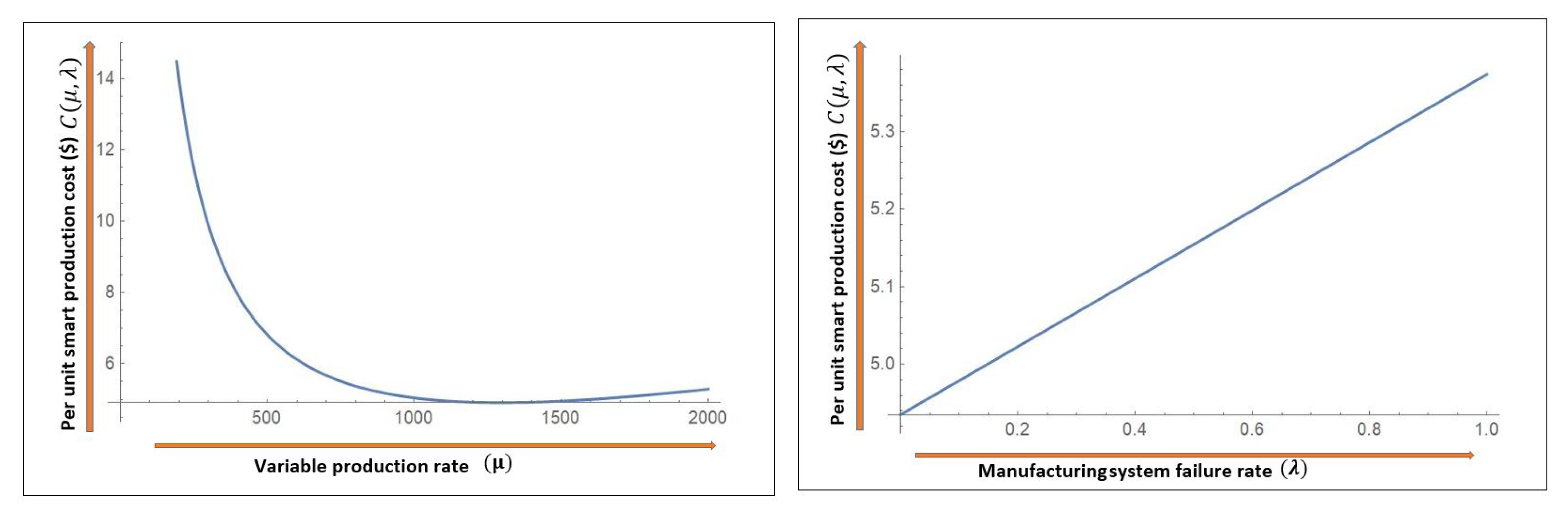
• The $c_{\mu }$ component represents the manufacturing costs, i.e., energy and lobar, and as the production rate increases, the manufacturing cost is equally distributed over a large number of the produced unit. Consequently the per unit manufacturing cost decreases with high production rates.
• The next cost component is $Y\lambda$, which represents the manufacturing yield loss. As the failure rate increases, the downtime increases and the overall costs of system increases. However, with higher production rates, the unit yield loss cost decreases.
• The last cost component is referred to as the tool/die cost, and it is directly proportional to production rate.

We consider an unreliable manufacturing system, which is subjected to random breakdowns. Whenever a breakdown occurs, the machine is assumed to immediately be under repair and an abort/resume inventory control policy is adopted. Under this inventory control policy, production of the interrupted lot resumes immediately after the machine is fixed and restored.

3.2. Assumptions

Given are the assumptions considered to develop this model.

-

An automated smart integrated production maintenance policy for an unreliable manufacturing system is considered.

-

The unreliability of a manufacturing system is modeled through a system performance-quality parameter which follows a stochastic process as discussed in [33].

-

The quality performance parameter of manufacturing system is expressed as a design variable, where it is represented as $\lambda =\frac{Totalnumberoffailure}{Totalworkinghours}$, and manufacturing quality performance can be increased through investment in advanced production technology and resources.

-

During production up-time $t_{\mu }$ system failure may occurs randomly, a single-machine and single-product type environment is considered.

-

Random failure rate and random repair rate is considered with generalized distributions.

-

On manufacturing system failure, corrective repair is started immediately. After corrective repair, manufacturing system is restored back to the same initial operational condition with an extra cost $R_s\lambda$.

-

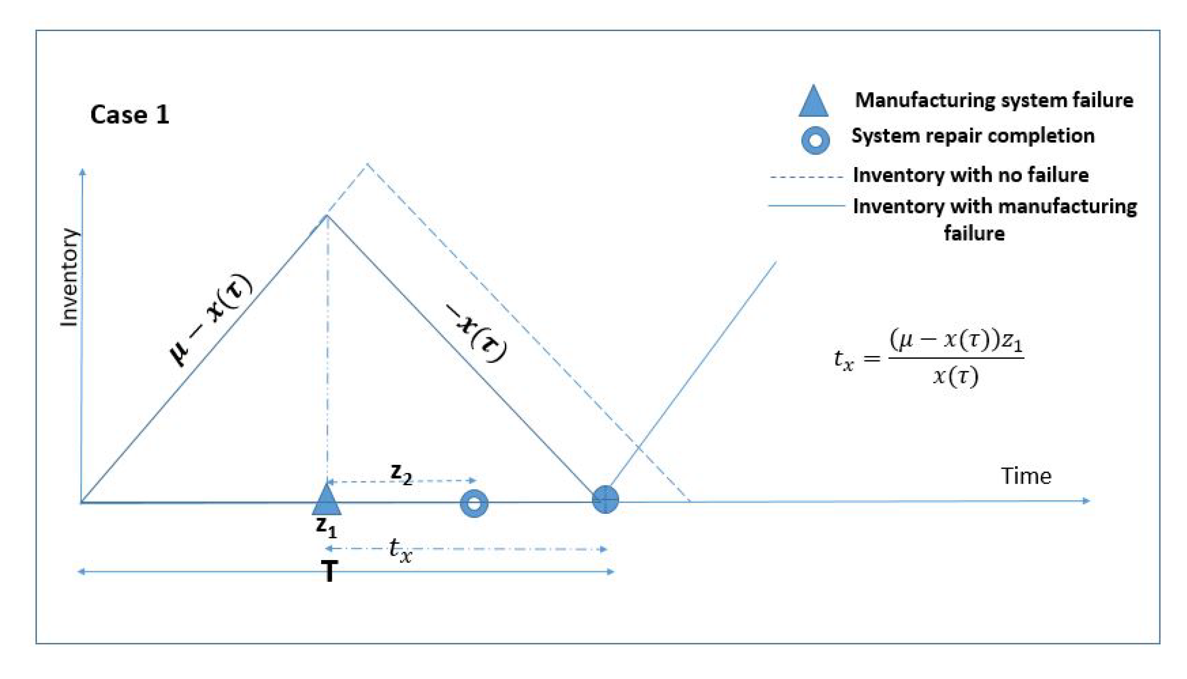
Upon manufacturing system breakdown, market demand is fulfilled from on-hand inventory, accumulated during production up-time.

-

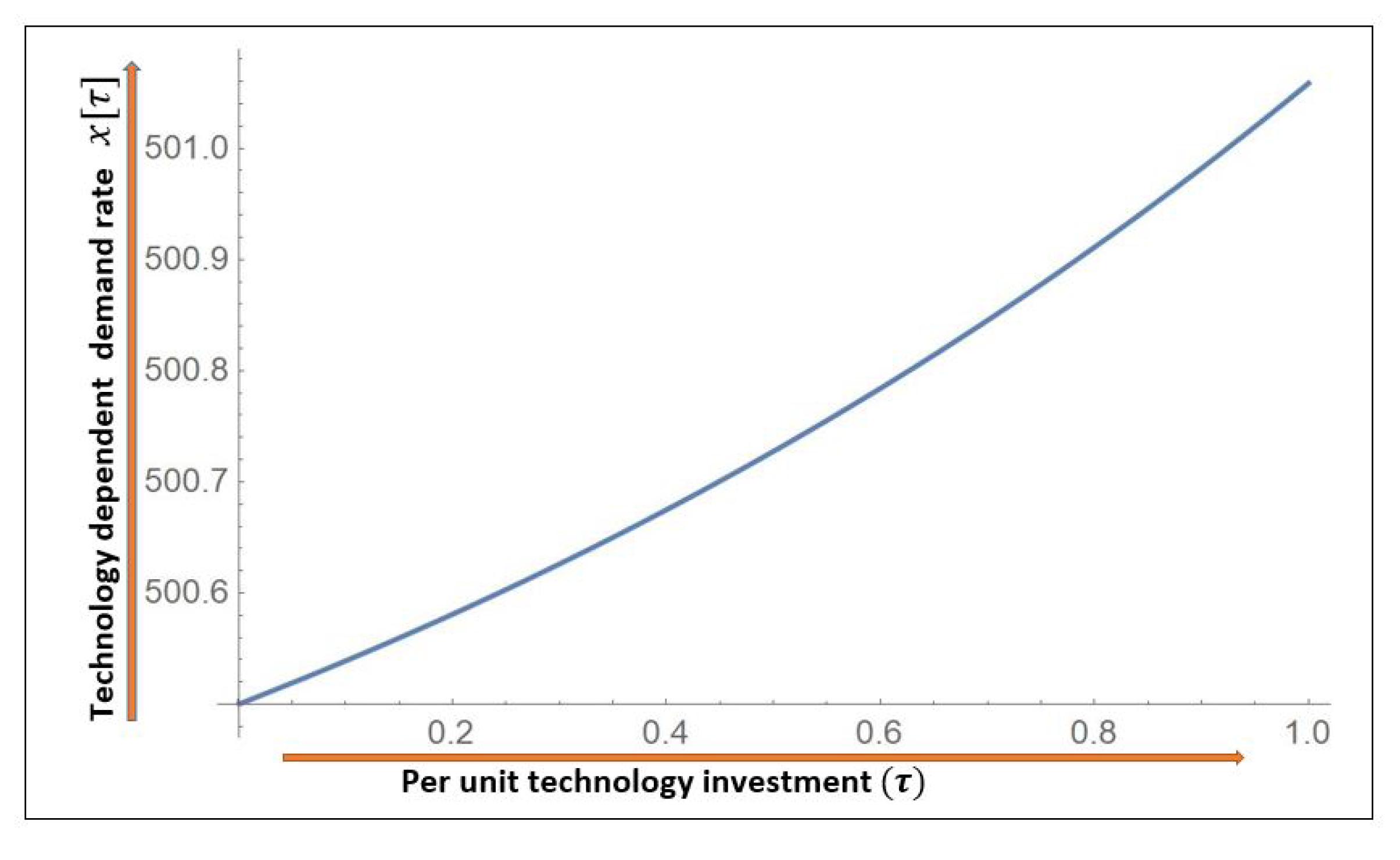
The demand is technology dependent as $(x\left[\tau \right]=a+\gamma e^{\eta \tau })$, where a is the potential market demand, $\eta$ is a shape parameter and it shows the effectiveness of product technology $\tau$, whereas $\gamma$ is a scale parameter. Moreover $\tau$ per unit technology investment is a decision variable and $\gamma ,\eta >0$.

-

If the on-hand inventory is sufficient to met market demand, then new production cycle is started after complete inventory consumption.

-

Market demand is a variable parameter and depend on technology investment $\tau$, where $\tau$ is a decision variable.

-

The production rate $\mu$ of smart manufacturing system is a controllable variable and can be varied within given limits $(\mu \in [{\mu }_{min}$$,{\mu }_{max}\left]\right)$. Moreover, the variable production rate is always greater than the variable demand rate as $({\mu }_{min}\ge x\left[\tau \right])$.

-

Unit smart production cost is a function of manufacturing quality performance parameter $\lambda$, manufacturing yield Y and variable production rate $\mu$.

-

The raw material cost linearly depends on the manufacturing quality performance parameter variable $\lambda$, i.e., ($r_1+r_2\lambda$).

-

As the manufacturing quality performance parameter decreases, the manufacturing yield loss increases, such that higher downtime increases system costs.

-

A shortage cost is considered for lost sales due to longer repair times.

4. Mathematical Model

The study investigated an integrated production maintenance model where the manufacturing system starts production at $(t=0)$ at a controllable production rate $\left(\mu ϵ\right[{\mu }_{min},$${\mu }_{max}\left]\right)$, to produce a lot size Q. The inventory piles up at the rate $(\mu \ast t_{\mu })$ until breakdown occurs. The on-hand inventory is formulated with a governing differential equation at the initial condition $I_1\left(0\right)=0$ as;

$$\begin{array}{c}\hfill \frac{{dI}_1\left(t\right)}{dt}=\mu -x\left[\tau \right](0\le t\le t_{\mu })\end{array}$$

(6)

The on-hand inventory is formulated with a governing differential equation with the given condition $I_1\left(t_{\mu }\right)=I_2\left(t_{\mu }\right)$ as;

$$\begin{array}{c}\hfill \frac{{dI}_2\left(t\right)}{dt}=-x\left[\tau \right](t_{\mu }\le t\le Z)\end{array}$$

(7)

The accumulated result of above equations gives,

$$\begin{array}{c}\hfill I\left(t\right)=\left(\begin{array}{cc}(\mu -x[\tau \left]\right)t& 0\le t\le t_{\mu }\\ {\mu \ast z}_1-x\left[\tau \right]t& t_{\mu }\le t\le Z\end{array}\right)\end{array}$$

(8)

Let t denotes the time before a breakdown take place and $t_{\mu }$ stands for the production up-time. Since during production up-time $t_{\mu }$ machine breakdown may occur randomly, if time to breakdown is $(t<t_{\mu })$, then a random breakdown occurs during the production up-time; if $(t\ge t_{\mu })$, then no breakdowns happen during the production up-time. Therefore, the following two separate situations should be examined.

4.1. Model 1: Random Production Rate Model with Breakdown

In the first case, production starts at ($t=0$) but at some random time $(t=z_1)$ the manufacturing system faces a break down before the completion of production at time ($t=t_{\mu }$). Therefore, inventory accumulates within interval $[0,z_1]$, and depletes in interval $[z_1,Z]$ with market demand rate $x\left[\tau \right]$. Hence, the total inventory becomes,

$$\begin{array}{c}\hfill {\int }_0^{z_1}(\mu -x\left[\tau \right])tdt+{\int }_{z_1}^Z\left({\mu z}_1-x\left[\tau \right]t\right)dt.\end{array}$$

(9)

After breakdown at time $(t=z_1)$, the manufacturing system undergoes corrective repair but due to the stochastic nature of repair rate, two additional inventory states may happen as given;

4.1.1. Case 1 ( Repair Time Lies within $\frac{z_1(\mu -x\left[\tau \right])}{x\left[\tau \right]}$ )

If the expected time to repair manufacturing system is short enough that it extends within a $\frac{z_1(\mu -x\left[\tau \right])}{x\left[\tau \right]}$ as shown in Figure 4, then the production quantity becomes,

$$\begin{array}{ccc}\hfill Q_1& =& {\int }_0^{\frac{Q}{\mu }}\left({\int }_0^{\frac{z_1(\mu -x\left[\tau \right])}{x\left[\tau \right]}}\mu z_{1}g\left(z_2\right)d{z}_2\right)g\left(z_1\right)d{z}_1.\hfill \end{array}$$

(10)

No shortages occur and expected inventory is equal to,

$$\begin{array}{ccc}\hfill I_1& =& {\int }_0^{\frac{Q}{\mu }}\left({\int }_0^{\frac{z_1(\mu -x\left[\tau \right])}{x\left[\tau \right]}}\left(\frac{\mu z_1^2(\mu -x\left[\tau \right])}{2x\left[\tau \right]}\right)g\left(z_2\right)d{z}_2\right)g\left(z_1\right)d{z}_1.\hfill \end{array}$$

(11)

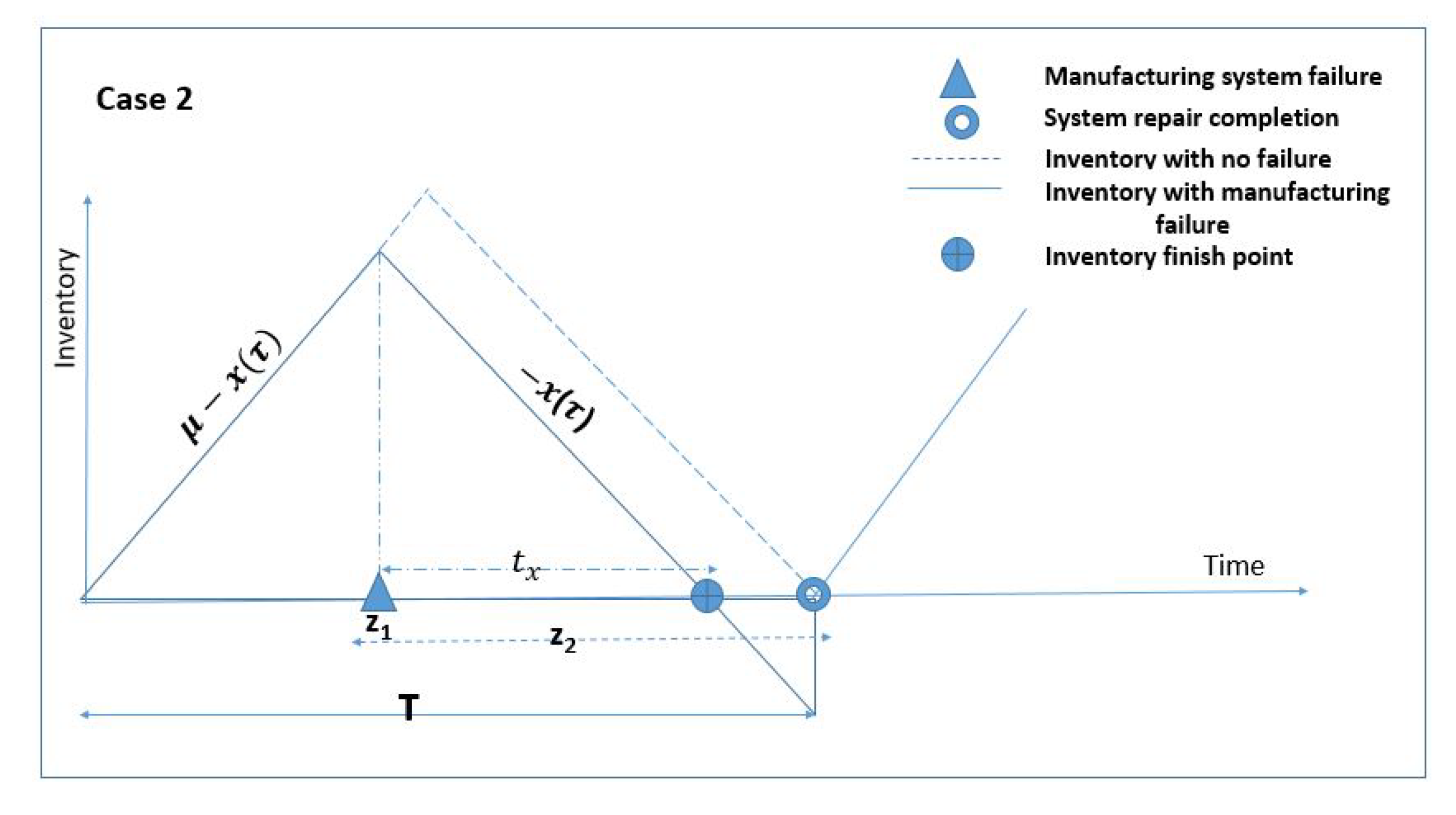
4.1.2. Case 2 (Repair Time Exceeds $\frac{z_1(\mu -x\left[\tau \right])}{x\left[\tau \right]}$)

If the expected time to repair manufacturing system exceeds $\frac{z_1(\mu -x\left[\tau \right])}{x\left[\tau \right]}$, see Figure 5, then the production quantity becomes,

$$\begin{array}{ccc}\hfill Q_2& =& \left.{\int }_0^{\frac{Q}{\mu }}\right({\int }_{\frac{z_1(\mu -x\left[\tau \right])}{x\left[\tau \right]}}^{\infty }\mu z_{1}g\left(z_2\right)d{z}_2)g\left(z_1\right)d{z}_1.\hfill \end{array}$$

(12)

Moreover the expected inventory is given as,

$$\begin{array}{ccc}\hfill I_2& =& {\int }_0^{\frac{Q}{\mu }}\left({\int }_{\frac{z_1(\mu -x\left[\tau \right])}{x\left[\tau \right]}}^{\infty }\left(\frac{\mu z_1^2(\mu -x\left[\tau \right])}{2x\left[\tau \right]}\right)g\left(z_2\right)d{z}_2\right)g\left(z_1\right)d{z}_1.\hfill \end{array}$$

(13)

The inventory holding cost

The expected average inventory for Model-1 is given in Equation (14) where expected cumulative inventory holding cost is $h_c{I}^1$.

$$\begin{array}{c}{I}^1={\int }_0^{\frac{Q}{\mu }}\left({\int }_0^{\frac{z_1(\mu -x\left[\tau \right])}{x\left[\tau \right]}}\left(\frac{\mu z_1^2(\mu -x\left[\tau \right])}{2x\left[\tau \right]}\right)g\left(z_2\right)d{z}_2+{\int }_{\frac{z_1(\mu -x\left[\tau \right])}{x\left[\tau \right]}}^{\infty }\left(\frac{\mu z_1^2(\mu -x\left[\tau \right])}{2x\left[\tau \right]}\right)g\left(z_2\right)d{z}_2\right)\hfill \\ g\left(z_1\right)d{z}_1.\hfill \end{array}$$

(14)

The smart production cost

The expected average production cost for Model-1 becomes,

$$\begin{array}{c}{C}^1(\mu ,\lambda )={\int }_0^{\frac{Q}{\mu }}\left({\int }_0^{\frac{z_1(\mu -x\left[\tau \right])}{x\left[\tau \right]}}\right.\left(\frac{c_{\mu }+Y\lambda }{\mu }+r_1+\mu \pi +r_2\lambda \right)\mu z_{1}g\left(z_2\right)d{z}_2+{\int }_{\frac{z_1(\mu -x\left[\tau \right])}{x\left[\tau \right]}}^{\infty }(\frac{c_{\mu }+Y\lambda }{\mu }\hfill \\ +r_1+\mu \pi +r_2\lambda \left)\mu z_{1}g\left(z_2\right)d{z}_2\right)g\left(z_1\right)d{z}_1.\hfill \end{array}$$

(15)

The shotage cost

The shortages during repair time are given as,

$$\begin{array}{c}{\int }_0^{\frac{Q}{\mu }}\left({\int }_{\frac{z_1(\mu -x\left[\tau \right])}{x\left[\tau \right]}}^{\infty }\left(z_{2}x\left[\tau \right]-z_1(\mu -x\left[\tau \right])\right)g\left(z_2\right)d{z}_2\right)g\left(z_1\right)d{z}_1.\hfill \end{array}$$

(16)

The set up cost

The setup cost for proposed model consists of two components, a fixed cost component for production, and a variable cost component which depends on the reliability parameter of the manufacturing system. As the failure rate increases, the setup cost increases with a certain amount of $R_s\lambda$ required for system restoration.

$$\begin{array}{c}\hfill S(1+R_s\lambda ).\end{array}$$

(17)

The system repair cost

Every time manufacturing system faces a breakdown, a corrective repair is carried down which results in a repair cost given as below,

$$\begin{array}{c}\hfill R_r{\int }_0^{\frac{Q}{\mu }}\left({\int }_0^{\infty }{z}_{2}g\left(z_2\right)d{z}_2\right)g\left(z_1\right)d{z}_1).\end{array}$$

(18)

The total smart production inventory cost per cycle $E\left[C_1\right]$ for Model-1 gained through combining the two cases consists of the setup cost, smart production technology development cost, variable production costs, variable repair cost, variable restoration cost, inventory holding costs, and shortage cost as given below;

$$\begin{array}{c}E[C_1(Q,\mu ,\lambda ,\tau )]=S(1+R_s\lambda )+\chi e^{\frac{\zeta \lambda }{\varrho }}+R_r{\int }_0^{\frac{Q}{\mu }}\left({\int }_0^{\infty }{z}_{2}g\left(z_2\right)d{z}_2\right)g\left(z_1\right)d{z}_1)+{\int }_0^{\frac{Q}{\mu }}\left({\int }_0^{\frac{z_1(\mu -x\left[\tau \right])}{x\left[\tau \right]}}\mu z_1\right.\hfill \\ \left.\left(\frac{c_{\mu }+Y\lambda }{\mu }+r_1+\mu \pi +r_2\lambda \right)g\left(z_2\right)d{z}_2\right)g\left(z_1\right)d{z}_1+\left.{\int }_0^{\frac{Q}{\mu }}\right(\left.{\int }_{\frac{z_1(\mu -x\left[\tau \right])}{x\left[\tau \right]}}^{\infty }(\mu z_1\left(\frac{c_{\mu }+Y\lambda }{\mu }+r_1+\mu \pi +r_2\lambda \right)\right)\hfill \\ g\left(z_2\right)d{z}_2)g\left(z_1\right)d{z}_1+h_c{\int }_0^{\frac{Q}{\mu }}\left({\int }_0^{\frac{z_1(\mu -x\left[\tau \right])}{x\left[\tau \right]}}\left(\frac{\mu z_1^2(\mu -x\left[\tau \right])}{2x\left[\tau \right]}\right)g\left(z_2\right)d{z}_2\right)g\left(z_1\right)d{z}_1+h_c{\int }_0^{\frac{Q}{\mu }}({\int }_{\frac{z_1(\mu -x\left[\tau \right])}{x\left[\tau \right]}}^{\infty }\hfill \\ \left(\frac{\mu z_1^2(\mu -x\left[\tau \right])}{2x\left[\tau \right]}\right)g\left(z_2\right)d{z}_2)g\left(z_1\right)d{z}_1+S_c{\int }_0^{\frac{Q}{\mu }}\left({\int }_{\frac{z_1(\mu -x\left[\tau \right])}{x\left[\tau \right]}}^{\infty }\left(z_{2}x\left[\tau \right]-z_1(\mu -x\left[\tau \right])\right)g\left(z_2\right)d{z}_2\right.)g\left(z_1\right)\hfill \\ d{z}_1.\hfill \end{array}$$

(19)

The cycle length is defined as the time interval between two successive production runs. Hence, the expected cycle length for Model-1 with stochastic failure and repair rate becomes,

$$\begin{array}{c}E\left[Z_1(Q,\mu ,\lambda ,\tau )\right]={\int }_0^{\frac{Q}{\mu }}\left({\int }_0^{\frac{z_1(\mu -x\left[\tau \right])}{x\left[\tau \right]}}\left(\frac{\mu z_1}{x\left[\tau \right]}\right)g\left(z_2\right)d{z}_2\right)g\left(z_1\right)d{z}_1+{\int }_0^{\frac{Q}{\mu }}({\int }_{\frac{z_1(\mu -x\left[\tau \right])}{x\left[\tau \right]}}^{\infty }\\ (z_1+z_2)g\left(z_2\right)d{z}_2)g\left(z_1\right)d{z}_1.\end{array}$$

(20)

4.2. Model 2: Random Production Rate Model without Breakdown

In this case, the production time before a manufacturing system failure taking place is greater than the production up-time, as $(t\ge t_{\mu })$, so there is no breakdown taking place during production run. Hence, the total smart production inventory costs per cycle $E\left[C_2\right]$ for Model-2 consists of setup costs, smart production technology development cost, variable production cost, and inventory holding cost.

$$\begin{array}{c}E\left[C_2(Q,\mu ,\lambda ,\tau )\right]=S+\chi e^{\frac{\zeta \lambda }{\varrho }}+h_c{\int }_{\frac{Q}{\mu }}^{\infty }\left(\frac{Q^2(\mu -x\left[\tau \right])}{2\mu x\left[\tau \right]}\right)g\left(z_1\right)d{z}_1+{\int }_{\frac{Q}{\mu }}^{\infty }\left(Q\left(\frac{c_{\mu }+Y\lambda }{\mu }+\mu \pi \right.\right.\hfill \\ +(r_1+r_2\lambda )\left)\right)g\left(z_1\right)d{z}_1.\hfill \end{array}$$

(21)

Similarly, the mean time length of production inventory cycle for the Model-2 is obtained as,

$$\begin{array}{c}\hfill E\left[Z_2(Q,\mu ,\lambda ,\tau )\right]={\int }_{\frac{Q}{\mu }}^{\infty }\left(\frac{Q}{x\left[\tau \right]}\right)g\left(z_1\right)d{z}_1.\end{array}$$

(22)

4.3. Integration of the EPQ Models with/without Failure

The expected total costs of smart manufacturing system per cycle is the sum of Model-1 and Model-2 and is given as;

$$\begin{array}{c}E\left[TC(Q,\mu ,\lambda ,\tau )\right]=S+R_s\lambda S+\chi e^{\frac{\zeta \lambda }{\varrho }}+R_r{\int }_0^{\frac{Q}{\mu }}\left({\int }_0^{\infty }{z}_{2}g\left(z_2\right)d{z}_2\right)g\left(z_1\right)d{z}_1+{\int }_0^{\frac{Q}{\mu }}({\int }_0^{\frac{z_1(\mu -x\left[\tau \right])}{x\left[\tau \right]}}\mu z_1\hfill \\ \left(\frac{c_{\mu }+Y\lambda }{\mu }+r_1+\mu \pi +r_2\lambda \right)g\left(z_2\right)d{z}_2)g\left(z_1\right)d{z}_1+{\int }_0^{\frac{Q}{\mu }}({\int }_{\frac{z_1(\mu -x\left[\tau \right])}{x\left[\tau \right]}}^{\infty }\mu z_1\left(\frac{c_{\mu }+Y\lambda }{\mu }+r_1+\mu \pi +r_2\lambda \right)\hfill \\ g\left(z_2\right)d{z}_2)g\left(z_1\right)d{z}_1+{\int }_{\frac{Q}{\mu }}^{\infty }\left(\left(\frac{c_{\mu }+Y\lambda }{\mu }+\mu \pi +r_1+\right.\right.r_2\lambda )Q)g\left(z_1\right)d{z}_1+h_c{\int }_0^{\frac{Q}{\mu }}({\int }_0^{\frac{z_1(\mu -x\left[\tau \right])}{x\left[\tau \right]}}\mu z_1^2\hfill \\ \left(\frac{(\mu -x[\tau \left]\right)}{2x\left[\tau \right]}\right)g\left(z_2\right)d{z}_2)g\left(z_1\right)d{z}_1+h_c{\int }_0^{\frac{Q}{\mu }}\left({\int }_{\frac{z_1(\mu -x\left[\tau \right])}{x\left[\tau \right]}}^{\infty }\left(\frac{\left.\mu z_1^2(\mu -x\left[\tau \right]\right)}{2x\left[\tau \right]}\right)g\left(z_2\right)d{z}_2\right)g\left(z_1\right)d{z}_1+h_c\hfill \\ {\int }_{\frac{Q}{\mu }}^{\infty }\left(\frac{Q^2(\mu -x\left[\tau \right])}{2\mu x\left[\tau \right]}\right)g\left(z_1\right)d{z}_1+S_c{\int }_0^{\frac{Q}{\mu }}\left({\int }_{\frac{z_1(\mu -x\left[\tau \right])}{x\left[\tau \right]}}^{\infty }\left(z_{2}x\left[\tau \right]-z_1(\mu -x\left[\tau \right])\right)g\left(z_2\right)d{z}_2\right)g\left(z_1\right)d{z}_1.\hfill \end{array}$$

(23)

Similarly the expected total cycle length of smart manufacturing system becomes,

$$\begin{array}{ccc}\hfill E\left[Z\right(Q,\mu ,\lambda ,\tau \left)\right]& =& {\int }_0^{\frac{Q}{\mu }}\left({\int }_0^{\frac{z_1(\mu -x\left[\tau \right])}{x\left[\tau \right]}}\left(\frac{\mu z_1}{x\left[\tau \right]}\right)g\left(z_2\right)d{z}_2\right)g\left(z_1\right)d{z}_1+{\int }_{\frac{Q}{\mu }}^{\infty }\left(\frac{Q}{x\left[\tau \right]}\right)g\left(z_1\right)d{z}_1.\hfill \end{array}$$

(24)

Owing to assumptions of stochastic failure and stochastic repair time distributions, the cycle length in the proposed model is a variable parameter. Therefore, the total expected cost per unit time in the steady state is driven using the renewal reward theorem [65],

$$\begin{array}{c}\hfill ETC[Q,\mu ,\lambda ,\tau ]=\frac{E_{z_1}\left[E_{z_2}\left[TC(Q,\mu ,\lambda ,\tau )\right]\right]}{E_{z_1}\left[E_{z_2}\left[Z(Q,\mu ,\lambda ,\tau )\right]\right]}\end{array}$$

(25)

With exponential distribution functions of smart manufacturing system failure and repair time, such that,

$$\begin{array}{c}\hfill G\left(z_1\right)=(1-e^{-\lambda z_1}),G\left(z_2\right)=(1-e^{-\theta z_2}).\end{array}$$

(26)

Thus using theses distributions given in Equation (26), the expected total cost derived in Equationa (23) and expected total cycle length derived in Equation (24) becomes

$$\begin{array}{cc}E[TC\hfill & (Q,\mu ,\lambda ,\tau )]=S+R_s\lambda S+\chi e^{\frac{\zeta \lambda }{\varrho }}+\frac{R_r}{\theta }(1-e^{-\frac{Q\lambda }{\mu }})+(c_{\mu }+Y\lambda +\mu ((r_1+r_2\lambda )+\mu \pi ))\\ & +\frac{e^{-\frac{Q\lambda }{\mu }}\left(e^{\frac{Q\lambda }{\mu }}-1\right)}{\lambda }+S_c\left(\lambda {\left(a+\gamma e^{\eta \tau }\right)}^2\right)\frac{e^{\frac{Q\left(-\frac{\mu \theta }{a+\gamma e^{\eta \tau }}+\theta -\lambda \right)}{\mu }}-1}{\theta \left(a(\theta -\lambda )+\gamma e^{\eta \tau }(\theta -\lambda )-\mu \theta \right)}+h_c\hfill \\ & \left(\frac{\left(\mu -\left(a+\gamma e^{\eta \tau }\right)\right)}{{\lambda }^2\left(a+\gamma e^{\eta \tau }\right)}\right)e^{-\frac{Q\lambda }{\mu }}\left(\mu \left(e^{\frac{Q\lambda }{\mu }}-1\right)-Q\lambda \right)\hfill \end{array}$$

(27)

and $E\left[Z\right(Q,\mu ,\lambda ,\tau \left)\right]$ becomes,

$$\begin{array}{c}E\left[Z\right(Q,\mu ,\lambda ,\tau \left)\right]=\frac{e^{Q\left(-\frac{\theta }{a+\gamma e^{\eta \tau }}-\frac{\lambda }{\mu }\right)}}{\left(\theta \lambda \left(a+\gamma e^{\eta \tau }\right)((\theta -\lambda )\left(a+\gamma e^{\eta \tau }\right)-\mu \theta )\right)}({\lambda }^2{\left(a+\gamma e^{\eta \tau }\right)}^2+\mu {\theta }^2\left(\mu -a-\gamma e^{\eta \tau }\right)\hfill \\ +\mu \theta \lambda \left(a+\gamma e^{\eta \tau }\right))\hfill \end{array}$$

(28)

4.4. Solution Methodology

The study considers production lot size Q, production rate $\mu$, reliability parameter $\lambda$, and per unit technology investment $\tau$ for products to be four decision variables. The expected total cost function is a non-linear constrained problem. Now, our objective is to minimize $E\left[TC\right(Q,\mu ,\lambda ,\tau \left)\right]$ under the constraints;

$$\begin{array}{cc}\hfill & -Q\le 0,\hfill \end{array}$$

(29)

$$\begin{array}{c}x\left[\tau \right]<\mu ,\hfill \end{array}$$

(30)

$$\begin{array}{c}\mu \le {\mu }_{max},\hfill \end{array}$$

(31)

$$\begin{array}{c}{\lambda }_{min}-\lambda \le 0,\hfill \end{array}$$

(32)

$$\begin{array}{c}\lambda -{\lambda }_{max}\le 0,\hfill \end{array}$$

(33)

$$\begin{array}{c}-\tau \le 0\hfill \end{array}$$

(34)

The Kuhn–Tucker method is used to solve provided non-linear constrained mathematical problem as KT Method is considered as an effective method to get global optimal solution [66,67]. Where, ${\beta }_1$, ${\beta }_2$, ${\beta }_3$, ${\beta }_4$, ${\beta }_5$, ${\beta }_6$ are considered the Lagrange multipliers corresponding to given constraints. Below given are KT conditions for optimal solution;

$$\begin{array}{c}\hfill \frac{\partial ETC[Q,\mu ,\lambda ,\tau ]}{\partial Q}+{\beta }_1=0,\frac{\partial ETC[Q,\mu ,\lambda ,\tau ]}{\partial \mu }-{\beta }_2+{\beta }_3=0,\end{array}$$

(35)

$$\begin{array}{c}\hfill \frac{\partial ETC[Q,\mu ,\lambda ,\tau ]}{\partial \lambda }-{\beta }_4+{\beta }_5=0,\frac{\partial ETC[Q,\mu ,\lambda ,\tau ]}{\partial \tau }+{\beta }_6=0.\end{array}$$

(36)

$$\begin{array}{c}\hfill {\beta }_{1}Q=0,{\beta }_6\tau =0,\end{array}$$

(37)

$$\begin{array}{c}\hfill {\beta }_2(x\left[\tau \right]-\mu )=0,{\beta }_3\left({\mu }_{max}-\mu \right)=0,\end{array}$$

(38)

$$\begin{array}{c}\hfill {\beta }_4\left(\lambda -{\lambda }_{max}\right)=0,{\beta }_5\left({\lambda }_{min}-\lambda \right)=0,\end{array}$$

(39)

$$\begin{array}{c}\hfill {\beta }_1,{\beta }_2,{\beta }_3,{\beta }_4,{\beta }_5,{\beta }_6\ge 0.\end{array}$$

(40)

The $ETC[Q,\mu ,\lambda ,\tau ]$ has the global optimal value at $Q^{*},{\mu }^{*},{\lambda }^{*},{\tau }^{*}$, if all principle minors ($H_1,H_2,H_3,H_4$) of Hessian matrix H should satisfy as ($H_1>0,H_2>0H_3>0H_4>0$). Where the generated Hessian matrix for ${ETC[Q,\mu ,\lambda ,\tau ]}^{*}$ is,

$$H=\left[\begin{array}{cccc}\frac{{\partial }^{2}ETC[Q,\mu ,\lambda ,\tau ]}{\partial Q^2}& \frac{{\partial }^{2}ETC[Q,\mu ,\lambda ,\tau ]}{\partial Q\partial \lambda }& \frac{{\partial }^{2}ETC[Q,\mu ,\lambda ,\tau ]}{\partial Q\partial \mu }& \frac{{\partial }^{2}ETC[Q,\mu ,\lambda ,\tau ]}{\partial Q\partial \tau }\\ \frac{{\partial }^{2}ETC[Q,\mu ,\lambda ,\tau ]}{\partial \lambda \partial Q}& \frac{{\partial }^{2}ETC[Q,\mu ,\lambda ,\tau ]}{\partial {\lambda }^2}& \frac{{\partial }^{2}ETC[Q,\mu ,\lambda ,\tau ]}{\partial \lambda \partial \mu }& \frac{{\partial }^{2}ETC[Q,\mu ,\lambda ,\tau ]}{\partial \lambda \partial \tau }\\ \frac{{\partial }^{2}ETC[Q,\mu ,\lambda ,\tau ]}{\partial \mu \partial Q}& \frac{{\partial }^{2}ETC[Q,\mu ,\lambda ,\tau ]}{\partial \mu \partial \lambda }& \frac{{\partial }^{2}ETC[Q,\mu ,\lambda ,\tau ]}{\partial {\mu }^2}& \frac{{\partial }^{2}ETC[Q,\mu ,\lambda ,\tau ]}{\partial \mu \partial \tau }\\ \frac{{\partial }^{2}ETC[Q,\mu ,\lambda ,\tau ]}{\partial \tau \partial Q}& \frac{{\partial }^{2}ETC[Q,\mu ,\lambda ,\tau ]}{\partial \tau \partial \lambda }& \frac{{\partial }^{2}ETC[Q,\mu ,\lambda ,\tau ]}{\partial \tau \partial \mu }& \frac{{\partial }^{2}ETC[Q,\mu ,\lambda ,\tau ]}{\partial {\tau }^2}\end{array}\right]$$

To prove the convexity of objective function, Appendix A is provided.

5. Numerical Experiment

The proposed model is examined with numerical analysis of model parameters. Furthermore, sensitivity analysis of the key input parameters is also provided. The modified values of input data are taken from [33,39] and are provided in

Table 2. General input parameter values for proposed model.

$r_1=1$ ($/unit)	$r_2=0.3$ ($/unit)	$S=2000$ ($/setup)
$Y=150$ ($)	$c_{\mu }=2500$ ($)	$R_s=0.0725$
$\pi =0.0015$	$R_r=500$ ($/unit  time)	$\theta =15$ (repairs /unit  time)
$S_c=5$ ($/unit)	$\zeta =1.02$	$\varrho =0.05$
$\chi =500$ ($)	$a=500$ (units/unit  time)	$\gamma =0.5$
$\eta =0.75$	$h_c=0.5$ ($/unit/unit  time)

.

The optimal results for decision variables of a developed integrated smart production maintenance policy for an unreliable manufacturing system are as follows, ${E\left[TC\right]}^{*}=3289.5(\$/\mathrm{unit}\mathrm{time}),Q^{*}=2985.27\left(\mathrm{units}\right)$ ${\mu }^{*}=1081.51\left(\mathrm{units}/\mathrm{unit}\mathrm{time}\right),{\tau }^{*}=0.006(\$/\mathrm{unit}),{\lambda }^{*}=5.54\times {10}^{-6}$.

Also, the Hessian matrix at optimal values of decision variables is a positive definite, as;

$$H=\left[\begin{array}{cccc}0.00009& -0.69& 0.0001& -0.0002\\ -0.69& 7.8\times {10}^6& -0.62& 2.04\\ 0.0001& -0.63& 0.0014& 2.59\times {10}^{-7}\\ -0.0002& 2.04& 2.6\times {10}^{-7}& 1.43\end{array}\right]$$

and all eigenvalues ($7.8\times {10}^6,1.44,0.0013,0.000085$) of the matrix are positive.

5.1. Sensitivity Analysis

This section studies the implications of reliability parameter, production lot size, production rate, and product technology investment on the integrated smart production maintenance model. To derive general insights into model drivers, a sensitivity analysis is performed and several meaningful results are drawn from the analysis that are given in subsequent discussions; see

Table 3. Sensitivity analysis for parameters related to manufacturing performance quality.

Parameter	Change	Q	$\mathit{\lambda }$	$\mathit{\mu }$	$\mathit{\tau }$	% Change in $\mathit{E}\left[\mathit{TC}\right]$
	%	(Units)	(Failures/Unit Time)	(Units/Unit Time)	($/Unit)	($/Unit/Unit Time)
$c_{\mu }$	−20	3424.64	$2.40\times {10}^{-8}$	0873.26	$3.2\times {10}^{-10}$	−7.92
	−10	3191.81	$2.19\times {10}^{-7}$	0983.87	$9.9\times {10}^{-16}$	−3.70
	+10	2977.92	$2.89\times {10}^{-7}$	1149.03	$8.5\times {10}^{-16}$	+3.07
	+20	2946.28	$2.00\times {10}^{-8}$	1203.95	$1.01\times {10}^{-14}$	+5.02
$r_1$	−20	3060.56	$8.88\times {10}^{-8}$	1075.18	$1.2\times {10}^{-13}$	−2.78
	−10	3060.64	$7.85\times {10}^{-8}$	1075.15	$1.2\times {10}^{-14}$	−1.54
	+10	3061.87	$8.30\times {10}^{-8}$	1074.71	$2.2\times {10}^{-16}$	+1.20
	+20	3145.10	$1.10\times {10}^{-8}$	1027.73	$8.7\times {10}^{-15}$	+2.77
$r_2$	−20	3059.87	$5.1\times {10}^{-8}$	1075.27	$4.4\times {10}^{-14}$	−0.11
	−10	3061.85	$1.2\times {10}^{-7}$	1074.72	$2.1\times {10}^{-13}$	−0.02
	+10	3074.20	$4.5\times {10}^{-8}$	1070.24	$3.6\times {10}^{-16}$	+0.01
	+20	3056.48	$2.1\times {10}^{-9}$	1075.55	$2.6\times {10}^{-10}$	+0.16
Y	−20	3059.92	$1.3\times {10}^{-7}$	1075.42	$9.1\times {10}^{-14}$	−0.02
	−10	3064.73	$2.2\times {10}^{-8}$	1073.37	$6.1\times {10}^{-15}$	−0.12
	+10	3088.96	$2.9\times {10}^{-8}$	1081.51	$8.2\times {10}^{-14}$	+0.15
	+20	inf	inf	inf	inf	inf
$\theta$	−20	3375.97	$1.0\times {10}^{-8}$	0975.35	$6.1\times {10}^{-14}$	+0.81
	−10	3058.88	$2.1\times {10}^{-8}$	1075.57	$1.2\times {10}^{-13}$	+0.004
	+10	3059.67	$2.8\times {10}^{-8}$	1075.51	$1.2\times {10}^{-10}$	−0.09
	+20	3066.45	$3.9\times {10}^{-8}$	1073.06	$1.9\times {10}^{-14}$	−0.11
$R_r$	−20	3058.21	$4.0\times {10}^{-8}$	1075.61	$1.4\times {10}^{-14}$	−0.01
	−10	3059.87	$2.8\times {10}^{-7}$	1075.43	$7.2\times {10}^{-16}$	−0.01
	+10	3058.48	$5.4\times {10}^{-8}$	1075.59	$6.3\times {10}^{-15}$	+0.01
	+20	3062.35	$4.0\times {10}^{-8}$	1074.54	$1.6\times {10}^{-15}$	+0.01
$\pi$	−20	2917.85	$1.1\times {10}^{-7}$	1214.58	$4.7\times {10}^{-13}$	−5.25
	−10	2998.08	$1.1\times {10}^{-7}$	1131.27	$1.8\times {10}^{-13}$	−2.28
	+10	3137.53	$1.2\times {10}^{-8}$	1019.07	$1.1\times {10}^{-13}$	+2.69
	+20	3214.55	$2.8\times {10}^{-7}$	0970.72	$3.7\times {10}^{-16}$	+4.65
$\gamma$	−20	3237.36	$6.5\times {10}^{-9}$	1012.05	$6.9\times {10}^{-13}$	−4.43
	−10	3059.23	$1.1\times {10}^{-7}$	1075.53	$4.6\times {10}^{-15}$	−0.02
	+10	3060.01	$9.0\times {10}^{-7}$	1075.48	$2.6\times {10}^{-15}$	+0.004
	+20	3063.44	$1.0\times {10}^{-7}$	1074.32	$1.1\times {10}^{-17}$	+0.004
$\eta$	−20	1916.47	$6.5\times {10}^{-9}$	1161.88	0.33	+2.68
	−10	3063.76	$4.9\times {10}^{-8}$	1074.20	$1.3\times {10}^{-15}$	+0.13
	+10	3066.49	$5.8\times {10}^{-8}$	1073.21	$3.6\times {10}^{-16}$	−0.07
	+20	inf	inf	inf	inf	inf
$S_c$	−20	3060.39	$8.2\times {10}^{-8}$	1075.25	$3.1\times {10}^{-14}$	−0.03
	−10	3059.60	$3.1\times {10}^{-8}$	1075.47	$3.3\times {10}^{-14}$	−0.03
	+10	3060.02	$4.0\times {10}^{-8}$	1075.38	$1.5\times {10}^{-12}$	−0.07
	+20	3062.40	$4.5\times {10}^{-8}$	1074.52	$1.6\times {10}^{-16}$	−0.07
$\chi$	−20	2993.77	$8.9\times {10}^{-8}$	1079.94	$1.8\times {10}^{-13}$	−0.51
	−10	3084.50	$4.5\times {10}^{-8}$	1056.75	$1.9\times {10}^{-15}$	−0.25
	+10	3093.58	$3.3\times {10}^{-7}$	1072.82	$1.2\times {10}^{-15}$	+0.24
	+20	3126.98	$4.1\times {10}^{-7}$	1070.26	$1.4\times {10}^{-16}$	+0.48
$\zeta$	−20	3062.26	$9.0\times {10}^{-8}$	1074.57	$1.1\times {10}^{-15}$	−0.02
	−10	3059.98	$1.7\times {10}^{-7}$	1075.39	$4.6\times {10}^{-18}$	−0.01
	+10	inf	inf	inf	inf	inf
	+20	inf	inf	inf	inf	inf
$h_c$	−20	3384.03	$1.2\times {10}^{-8}$	1102.44	$2.3\times {10}^{-13}$	−2.85
	−10	3221.49	$2.3\times {10}^{-8}$	1077.35	$3.3\times {10}^{-15}$	−1.29
	+10	2966.62	$1.7\times {10}^{-8}$	1043.72	$5.4\times {10}^{-15}$	+1.21
	+20	2198.90	$3.6\times {10}^{-5}$	1108.43	0.04	+3.13
S	−20	2809.52	$4.5\times {10}^{-7}$	1094.69	$2.1\times {10}^{-14}$	−1.87
	−10	2939.03	$7.9\times {10}^{-8}$	1084.00	$1.1\times {10}^{-13}$	−0.95
	+10	3213.57	$4.6\times {10}^{-8}$	1061.55	$8.5\times {10}^{-15}$	+0.97
	+20	3356.06	$1.8\times {10}^{-8}$	1043.57	$3.2\times {10}^{-14}$	+1.93
$R_s$	−20	3067.79	$3.6\times {10}^{-8}$	1072.58	$1.4\times {10}^{-14}$	−0.07
	−10	3093.14	$2.4\times {10}^{-8}$	1063.56	$5.6\times {10}^{-14}$	−0.18
	+10	3062.60	$5.7\times {10}^{-8}$	1074.45	$1.5\times {10}^{-14}$	+0.003
	+20	3195.18	$1.1\times {10}^{-8}$	1016.47	$2.4\times {10}^{-16}$	+0.53

.

Production cost: As the per unit manufacturing cost $c_{\mu }$ decreases, production rate $\mu$ also decreases which eventually decreases the average expected total cost. For higher per unit production costs, the production lot size becomes smaller in every manufacturing system to decrease the total production cost. As the production lot size decreases, the reliability parameter also decreases because the manufacturing system faces smaller working states. For unit production cost variations, the per unit technology investment $\tau$ for products shows symmetrical behavior for both increment and decrement approaches, and it shows that higher investment in technology is not optimal when the production cost is minimal or already very high.

Raw material cost: As the raw material cost $r_1$ decreases, the total expected cost decreases, which is a common feature of production. The production lot and production rate increases with decreases in raw material cost. The reliability parameter $\lambda$ increases in a decreasing fashion with material cost reduction, because less valued products means less complex production processes, which reduces the machine stress and eventually failure rate of such manufacturing systems decreases which does not involve complex manufacturing processes. On the other hand, the technology investment cost increases with decreases in raw material cost, which shows that products with less value in terms of materialistic value have the potential for value increases with technology advancements. Because products with less materialistic values are usually not use for technical and advanced technology-based goods.

Raw material yield loss cost: As $r_2$ cost is linearly dependent on manufacturing reliability, the decrease in the value of this cost means, the yield loss has less contribution to production system total costs, so it leads to higher value of reliability parameter. As the yield loss cost increases to decreases the failure rate, so reduction in this cost linearly increase the failure rate. Also, production lot size decreases with increases in manufacturing unreliability to decrease the total expected cost of the system. The decrease in raw material yield loss value decreases the total expected cost of system, as it reduces the material loss value. The per unit technology investment for raw material yield loss cost shows quite a unique trend, as with the increases in the yield loss cost value, reliability parameter decreases, the optimal investment decreases, and in the opposite case when yield lost cost increases, the production lot increases but the optimal investment decreases to reduce total expected cost, and especially with a 20% increase in yield loss cost, the production lot increases in a decreasing fashion due to lower the value of the manufacturing reliability parameter. Manufacturing yield loss cost: As the value of the manufacturing yield loss Y decreases, the total expected cost decreases due to increased reliability and decreased failure rate. With the decrease in manufacturing yield loss, as the manufacturing system faces less downtime, production rate increases in a decreasing fashion. The investment in product technology increases as the production rate and reliability parameter increases with decrease in manufacturing yield loss. However, with an increase of 20%, the model shows an infeasible solution for high-tech production.

Number of repairs: As the $\theta$ decreases the mean time to repair increases. The less number of repairs per unit time, the higher downtime. The expected total cost of system increases with decrease in repair rate due to higher downtime and less productivity costs.

Repair cost: The change in repair cost $R_r$ have a greater effect on production lot size. The decrease in corrective repair cost of manufacturing system decreases the total expected cost of the system, which decreases the production rate and increases the production lot size to optimize the total cost of system. Product technology investment is also sensitive to a higher manufacturing system repair cost, as it suggests a decreases for investment amount. With the increase in repair cost, the reliability parameter value increases to adjust the production technology development cost to avoid higher costs of maintenance. A 20% increase in corrective maintenance costs suggest a lower value of the reliability parameter to maintain the total optimal cost of manufacturing system.

Demand parameters: As the value of $\eta$ reduces, the effectiveness of technology reduces, which optimizes the total cost required per unit investment, and overall the production quantity increases. The decreases in g also decreases production rate, which decreases the reliability parameter of manufacturing system. This parameter scales down the technology-based demand part, and as this value decreases, the effect of required investment increases to increase demand. As the demand increases with the reduction of scale down parameter, the production quantity increases and consequently the total expected cost increases. The scale down parameter is very sensitive to increments, as until a 10% increase, the total cost decreases despite the reduction in required investment and reliability parameter. Therefore, a decrease of 20% or more in per unit technology investment for products should be considered to reduce total expected cost for an unreliable manufacturing system. Smart production technology development cost: The production technology development investment $\chi$ is when ($\lambda ={\lambda }_{min}$), so as the system becomes more unreliable, the required investment in smart technology to increase its productivity, and reliability increases. In the case of this model, the change in investment shows quite diverse impacts because of the communal influence of different model parameters. As the required production technology investment decreases, it shows a more reliable system, so the failure rate decreases, which also decreases the total expected cost of the system. At this point the production lot size and production rate also increases to maintain the total expected cost at an optimal level. On the other hand, when the required technology investment increases, the reliability parameter increases to adjust the smart technology development cost at an optimal level. With increases in failure rate, the production rate of the model decreases, which increases the per unit smart production cost and hence the total expected cost of system increases. A 20% or more increase in smart production technology cost suggests less per unit technology investments for products to maintain the total expected cost, as for manufacturing systems where the cost for technological modification is very high, the changes in product technology leads to higher system costs.

$\zeta$ is the scale-up parameter for manufacturing reliability parameter; as the value of $\zeta$ decreases the, the required smart technology cost decreases and the total expected cost of system also decreases. The decreases in $\zeta$ increases the production lot size and production rate, but suggests a lower technology investment value for products. The higher values of $\zeta$ shows an infeasible solution for the proposed unreliable manufacturing system due to the implication of higher unreliability costs. $\varrho$ is the scale down parameter of the manufacturing reliability parameter, and as the value of $\varrho$ decreases, the required smart technology cost increases, and the total expected cost of system increases. As the decrease in $\varrho$ increases, the total expected cost of system, the production lot size, and production rate increases accordingly to adjust the optimal total expected cost of the system. The model suggests that a 10% increase in value of $\varrho$ leads to an infeasible solution, as at a 10% decrease, the reliability parameter decreases significantly to adjust the development cost, which accordingly leads to higher reliability costs.

Shortage cost: As the shortage per unit cost decreases, the total expected cost decreases. Here with the decrease in shortage cost, the production lot size increases, which is opposite to deterministic demand models. The reason behind this is the technology investment-dependent demand. The model suggests products for which the shortage cost is less, and such products generally are not high-tech/electronic products, so with less shortage cost, the model optimizes production cost with a decrease in technology investment which directly increases production quantity. Surprisingly, the changes in shortage cost show symmetric behavior for the total cost of the system due to a change in product technology investment. The increase in shortage cost decreases the total cost of the system with a reduction in smart production technology investment.

Inventory holding cost: The expected total model cost increases with an increase in inventory holding cost. To minimize the total cost in such a situation, the model increases the production rate with decreasing production quantity to reduce the total expected production cost. With the increase in unit holding cost, the reliability parameter is insensitive, whereas, the product technology investment reduces with increased inventory holding cost; this is also to compensate higher inventory costs for expensive high-tech products. So for high-tech products, the increase in inventory holding costs suggests a reduction in technology-investment for products.

OPT vs per unit technological investment:

Table 4. Sensitivity analysis for parameters related to manufacturing reliability $F\left(t\right)$ and product technology ($\tau$).

Parameter	%	$\mathit{Manufacturing}$	$\mathit{\lambda }$	$\mathit{C}(\mathit{\mu },\mathit{\lambda })$	$\mathit{\tau }$	% Change in $\mathit{E}\left[\mathit{TC}\right]$
	Change	$\mathit{Reliability}(\%)$	(Rate)	($/Unit/Unit Time)	($/Unit)	($/Unit/Unit Time)
$c_{\mu }$	−20	100	$2.40\times {10}^{-8}$	4.60	$3.2\times {10}^{-10}$	−7.92
	−10	99	$2.19\times {10}^{-7}$	4.70	$9.9\times {10}^{-16}$	−3.70
	+10	99	$2.89\times {10}^{-7}$	5.09	$8.5\times {10}^{-16}$	+3.07
	+20	100	$2.00\times {10}^{-8}$	5.20	$1.01\times {10}^{-14}$	+5.02
$r_1$	−20	99	$8.88\times {10}^{-8}$	4.75	$1.2\times {10}^{-13}$	−2.78
	−10	99	$7.85\times {10}^{-8}$	4.80	$1.2\times {10}^{-14}$	−1.54
	+10	100	$8.30\times {10}^{-8}$	5.01	$2.2\times {10}^{-16}$	+1.20
	+20	100	$1.10\times {10}^{-8}$	5.17	$8.7\times {10}^{-15}$	+2.77
$r_2$	−20	100	$5.1\times {10}^{-8}$	4.90	$4.4\times {10}^{-14}$	−0.11
	−10	99	$1.2\times {10}^{-7}$	4.93	$2.1\times {10}^{-13}$	−0.02
	+10	99	$4.5\times {10}^{-8}$	4.90	$3.6\times {10}^{-16}$	+0.01
	+20	100	$2.1\times {10}^{-9}$	4.93	$2.6\times {10}^{-10}$	+0.16
Y	−20	99	$1.3\times {10}^{-7}$	4.93	$9.1\times {10}^{-14}$	−0.02
	−10	99	$2.2\times {10}^{-8}$	4.94	$6.1\times {10}^{-15}$	−0.12
	+10	100	$2.9\times {10}^{-8}$	4.94	$8.2\times {10}^{-14}$	+0.15
	+20	inf	inf	inf	inf	inf
$\theta$	−20	100	$1.0\times {10}^{-8}$	5.03	$6.1\times {10}^{-14}$	+0.81
	−10	99	$2.1\times {10}^{-8}$	4.94	$1.2\times {10}^{-13}$	+0.004
	+10	100	$2.8\times {10}^{-8}$	4.93	$1.2\times {10}^{-10}$	−0.09
	+20	100	$3.9\times {10}^{-8}$	4.94	$1.9\times {10}^{-14}$	−0.11
$R_r$	−20	100	$4.0\times {10}^{-8}$	4.94	$1.4\times {10}^{-14}$	−0.01
	−10	99	$2.8\times {10}^{-7}$	4.94	$7.2\times {10}^{-16}$	−0.01
	+10	100	$5.4\times {10}^{-8}$	4.94	$6.3\times {10}^{-15}$	+0.01
	+20	100	$4.0\times {10}^{-8}$	4.94	$1.6\times {10}^{-15}$	+0.01
$\gamma$	−20	100	$6.5\times {10}^{-9}$	5.00	$6.9\times {10}^{-13}$	−4.43
	−10	99	$1.1\times {10}^{-7}$	4.94	$4.6\times {10}^{-15}$	−0.02
	+10	99	$9.0\times {10}^{-7}$	4.94	$2.6\times {10}^{-15}$	+0.004
	+20	99	$1.0\times {10}^{-7}$	4.94	$1.1\times {10}^{-17}$	+0.004
$\eta$	−20	99	$6.5\times {10}^{-9}$	4.89	0.33	+2.68
	−10	100	$4.9\times {10}^{-8}$	4.93	$1.3\times {10}^{-15}$	+0.13
	+10	100	$5.8\times {10}^{-8}$	4.94	$3.6\times {10}^{-16}$	−0.07
	+20	inf	inf	inf	inf	inf
$S_c$	−20	99	$8.2\times {10}^{-8}$	4.94	$3.1\times {10}^{-14}$	−0.03
	−10	100	$3.1\times {10}^{-8}$	4.94	$3.3\times {10}^{-14}$	−0.03
	+10	100	$4.0\times {10}^{-8}$	4.94	$1.5\times {10}^{-12}$	−0.07
	+20	100	$4.5\times {10}^{-8}$	4.94	$1.6\times {10}^{-16}$	−0.07
$\chi$	−20	99	$8.9\times {10}^{-8}$	4.94	$1.8\times {10}^{-13}$	−0.51
	−10	99	$4.5\times {10}^{-8}$	4.95	$1.9\times {10}^{-15}$	−0.25
	+10	99	$3.3\times {10}^{-7}$	4.94	$1.2\times {10}^{-15}$	+0.24
	+20	99	$4.1\times {10}^{-7}$	4.94	$1.4\times {10}^{-16}$	+0.48
$\zeta$	−20	99	$9.0\times {10}^{-8}$	4.93	$1.1\times {10}^{-15}$	−0.02
	−10	99	$1.7\times {10}^{-7}$	4.93	$4.6\times {10}^{-18}$	−0.01
	+10	inf	inf	inf	inf	inf
	+20	inf	inf	inf	inf	inf
$h_c$	−20	100	$1.2\times {10}^{-8}$	4.92	$2.3\times {10}^{-13}$	−2.85
	−10	100	$2.3\times {10}^{-8}$	4.94	$3.3\times {10}^{-15}$	−1.29
	+10	100	$1.7\times {10}^{-8}$	4.96	$5.4\times {10}^{-15}$	+1.21
	+20	99	$3.6\times {10}^{-5}$	4.91	0.04	+3.13
$\pi$	−20	99	$1.1\times {10}^{-7}$	4.52	$4.7\times {10}^{-13}$	−5.25
	−10	99	$1.1\times {10}^{-7}$	4.75	$1.8\times {10}^{-13}$	−2.28
	+10	99	$1.2\times {10}^{-8}$	5.13	$1.1\times {10}^{-13}$	+2.69
	+20	99	$2.8\times {10}^{-7}$	5.32	$3.7\times {10}^{-16}$	+4.65
S	−20	99	$4.5\times {10}^{-7}$	4.92	$2.1\times {10}^{-14}$	−1.87
	−10	100	$7.9\times {10}^{-8}$	4.93	$1.1\times {10}^{-13}$	−0.95
	+10	100	$4.6\times {10}^{-8}$	4.95	$8.5\times {10}^{-15}$	+0.97
	+20	100	$1.8\times {10}^{-8}$	4.96	$3.2\times {10}^{-14}$	+1.93
$R_s$	−20	100	$3.6\times {10}^{-8}$	4.93	$1.4\times {10}^{-14}$	−0.07
	−10	100	$2.4\times {10}^{-8}$	4.94	$5.6\times {10}^{-14}$	−0.18
	+10	100	$5.7\times {10}^{-8}$	4.94	$1.5\times {10}^{-14}$	+0.003
	+20	100	$1.1\times {10}^{-8}$	4.99	$2.4\times {10}^{-16}$	+0.53

. provides a comprehensive overview of unit cost per product, technological investment per item, manufacturing reliability, and reliability parameter of the production system. Along with the per-unit manufacturing cost $c_{\mu }$, the tool/die cost $\pi$ is another influential part of the production system affecting per unit production costs as it increases directly with a higher production rate $\mu$. With an increase of 20% in $\pi$, the model results highest $C(\mu ,\lambda )=\$5.32$. The second highest unit production cost of $\$5.17$ results due to a 20% increase in raw material cost. Also, for an unreliable manufacturing system, the study suggests the lowest technological investment per product with an increase in the technology scaling factor $\gamma$. The study infers the importance of performance quality parameter $\zeta$ for per-unit technological investment for products $\tau$, as even ab 10% increase in $\zeta$ gives unfeasible results for the proposed unreliable production model.

5.1.1. Comparative Study

As shown in Figure 6, as the production lot size increases, the total expected cost of the system decreases to an optimal value where the total cost is at a minimum; this is because the unit smart production cost is equally distributed over the optimal production lot size Q.

The graph shows that $E\left[TC\right(Q,\mu ,\lambda ,\tau \left)\right]$ is not monotonically decreasing in Q, as there exists an optimal production lot size Q, after which the total expected costs starts to increase with an increase in production quantity. Figure 7 depicts the effect of controllable production rate $\mu$ on the expected total cost of smart manufacturing system $E\left[TC\right(Q,\mu ,\lambda ,\tau \left)\right]$. With the increase in production rate, the expected total cost decreases to a certain limit, after which it starts to increase again. This analysis can be justified with the help of Figure 3, where when the production rate of smart manufacturing system increases the unit production cost decreases. consequently, the total cost of the system decreases until optimal production rate $\mu =1081.5$.

As shown in Figure 8, the expected total cost $E\left[TC\right(Q,\mu ,\lambda ,\tau \left)\right]$ monotonically increases with manufacturing unreliability. As the failure rate of smart manufacturing system increases, the total cost increases due to productivity loss and extra costs incurred due to repair and idle time.

Figure 9 presents the effects of technology investment in finished goods, although the technology increases the demand rate but it also increases the total cost, especially in the case of unreliable manufacturing system, the investment are extra costly for system. So, a trade-off should be considered between smart production technology investment and product technology investment.

Figure 10 illustrates the joint effects of production lot size and controllable production rate on the expected total cost of system, as the production lot size increases the total cost $E\left[TC\right(Q,\mu ,\lambda ,\tau \left)\right]$ of the system decreases, whereas in the case of controllable production rate, the cost of the unreliable manufacturing system decreases to a optimal limit after which the expected total cost $E\left[TC\right(Q,\mu ,\lambda ,\tau \left)\right]$ starts to increase. On the whole, at production lot size 2900–3000 and production rate 1000–1100, we see a minimum $E\left[TC\right(Q,\mu ,\lambda ,\tau \left)\right]$ cost for the system which gives the optimal values of lot size and production rate as ($Q=2985.27,\mu =1081.51$).

Figure 11 presents the joint effects of manufacturing reliability parameter and controllable production rate on expected total cost of system; as the manufacturing reliability parameter increases the total cost of the system increases as a result of additional maintenance, restoration costs, and lower productivity, whereas in the case of controllable production rate, the cost of an unreliable manufacturing system decreases to a optimal limit after which the total cost starts to increase.

On the whole, at manufacturing reliability parameter within limit ($0,<0.01$) and production rate 1000–1100, we see a minimum total cost for the system which gives the optimal values of reliability parameter and production rate as ($\lambda =<0.01,\mu =1081.51$).

Figure 12 presents the joint effects of manufacturing reliability parameter and high-tech investment per unit on the expected total cost of system, as the manufacturing reliability parameter increases the total cost of the system increases as a result of additional system cost, production technology development and reduced productivity, moreover in the case of technology investment per unit, the cost of unreliable manufacturing system increases linearly. On the whole, at manufacturing reliability parameter within limit ($0,<0.01$) and product technology investment less than 0.01, the total cost for the system stays minimum which gives optimal values of reliability parameter and technology investment per unit as ($\lambda =<0.01,\tau =<0.01$).

Figure 13 presents the joint effects of controllable production rate and high-tech investment per unit on expected total cost of system; as the production rate increases the total cost of the system decreases to a optimal limit after which it increases due to higher per unit production cost. Moreover, in the case of technology investment per unit, the cost of unreliable manufacturing system increases linearly. On the whole, at variable production rate within limit (1000–1100) and product technology investment less than 0.01, the total cost for the system stays minimum which gives optimal values of production rate and technology investment per unit as ($\mu =1081.51,\tau =<0.01$).

Figure 14 presents the joint effects of production lot size and high-tech investment per unit on expected total cost of system, andas the production lot size increases, the total cost of the system decreases to a optimal limit. Moreover, in the case of technology investment per unit, the cost of unreliable manufacturing system increases linearly. On the whole, at production lot size within limit (1000–4500) and product technology investment less than 0.01, the total cost for the system remains at a minimum which gives the optimal values of production rate and technology investment per unit as ($Q=2985.27,\tau =<0.01$).

Figure 15 presents the joint effects of production lot size and manufacturing reliability parameter on expected total cost of system, as the production lot size increases the total cost of the system decreases to a optimal limit, moreover in the case of reliability parameter, the cost of unreliable manufacturing system increases linearly. On the whole, at production lot size within limit (1000–4500) and reliability parameter value less than 0.01, the total cost for the system stays minimum which gives optimal values of production rate and reliability parameter as ($Q=2985.27,\lambda =<0.01$).

5.1.2. Managerial Insights

Some recommendations are provided for the industrial mangers as follows:

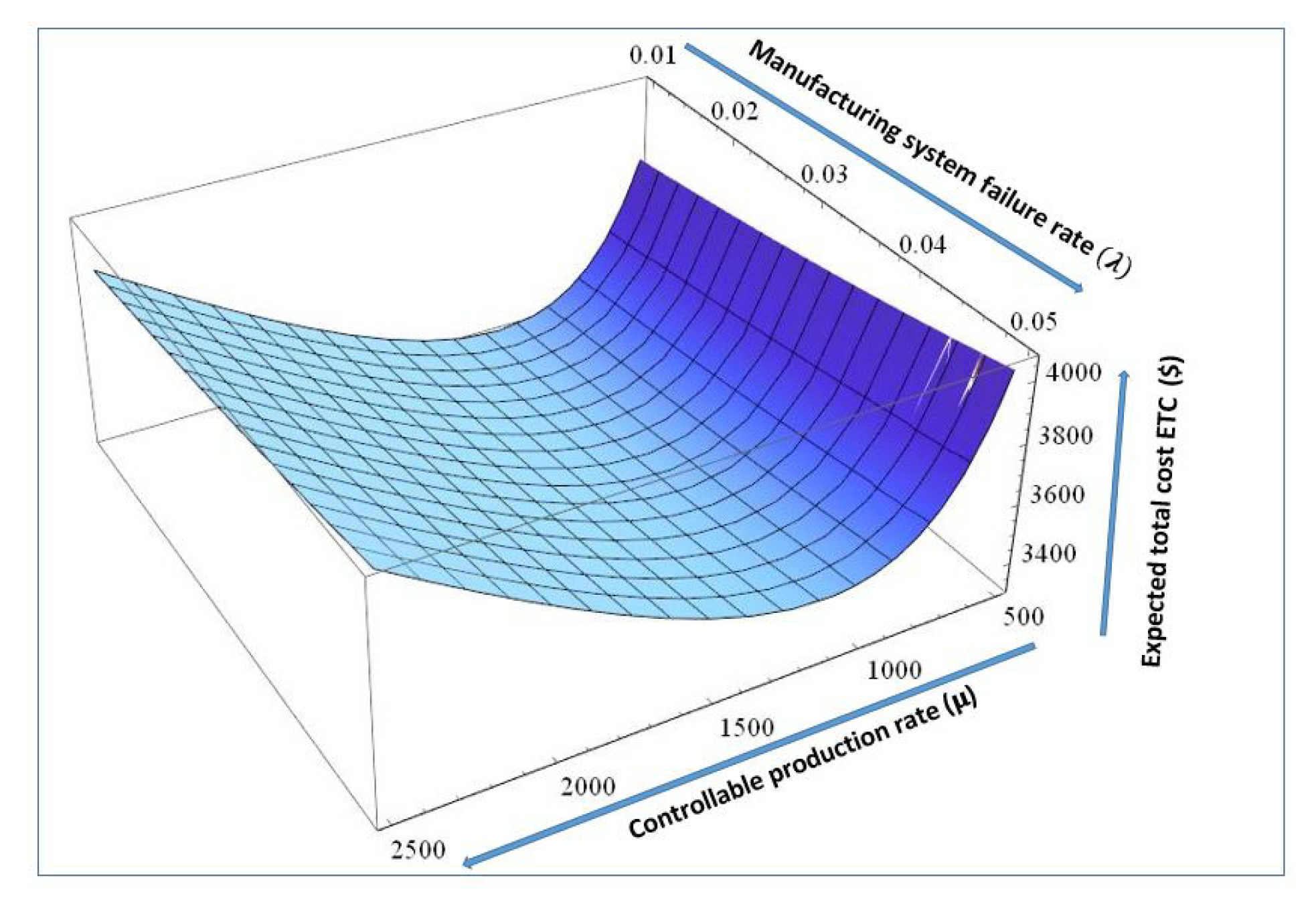
• The major insight for the industrial management is to assess uncertain production capacity for automated smart production planning. In a real world production environment, productivity and manufacturing efficiency is compromised generally because of an unreliable and limited production capacity system. Therefore, we provide comprehensive details for the influence of the reliability parameter on production rates and production capacity for optimal production planning.
• As the study is considered for a smart production inventory model, random breakdowns and random repair time is considered, therefore a production manager can easily do the calculations for optimal production quantity and optimal controllable production rates based on random system breakdowns in production planning.
• The unreliable manufacturing system provides optimum values for all decision variables, and if the manufacturing unit is producing smart products, for example high-tech products/electronic products, then our model provides the insight to choose investment options based on manufacturing system reliability.

6. Conclusions

This manuscript proposed a novel intelligent production maintenance model under stochastic manufacturing reliability for technology dependent demand and variable production rate. The study has extended a basic production inventory model with practical and realistic assumptions as follows:

-

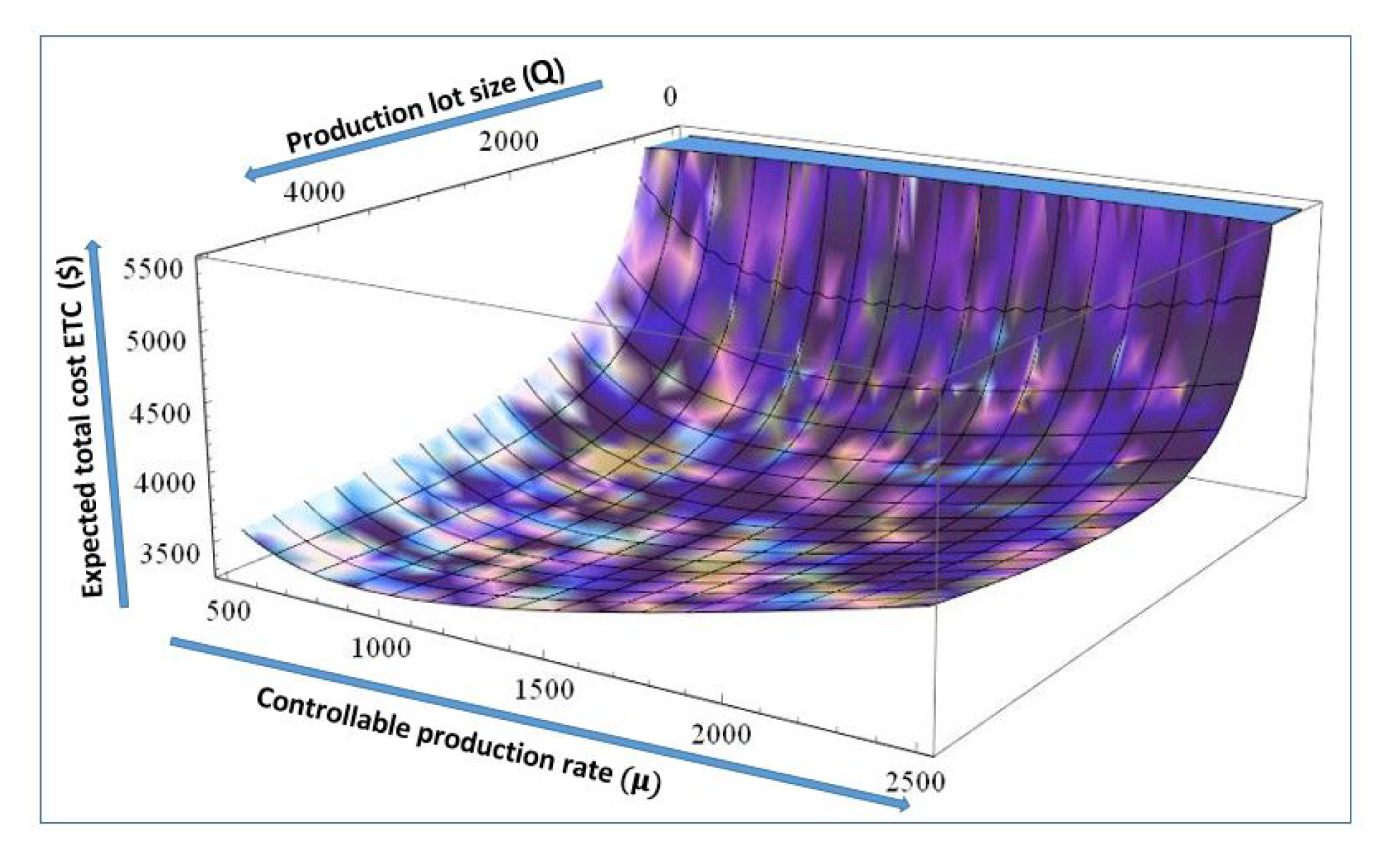
Rather than fixed designed production rates, the model considers a controllable production rate-based automated smart manufacturing system which reduces the per unit production cost. Along with the production rate $\mu$, the per unit production cost also depends on the manufacturing reliability and productivity parameter $\lambda$.

-

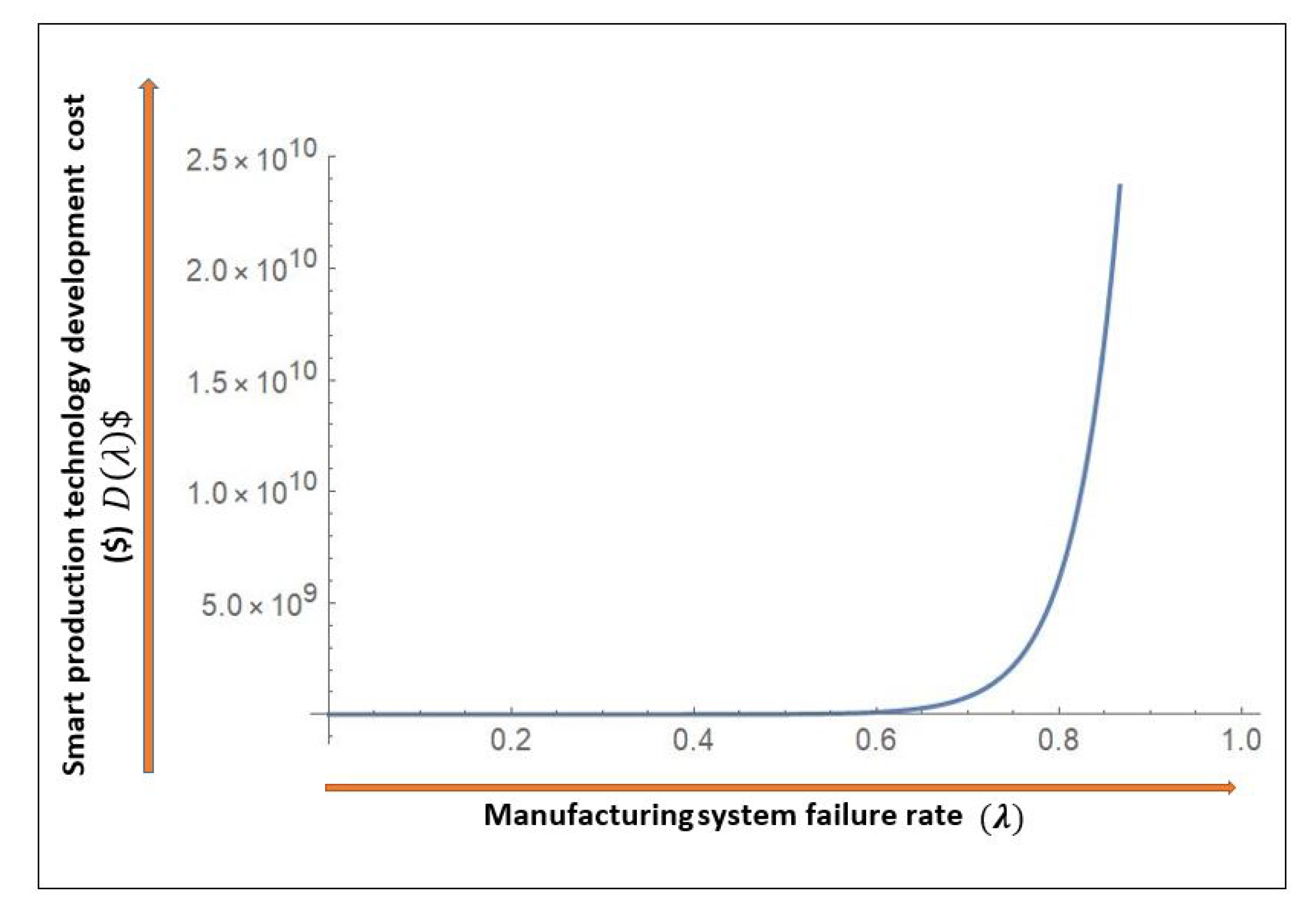
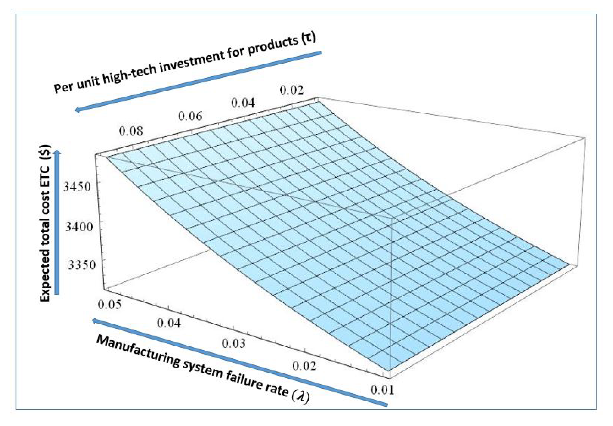
The manufacturing system productivity and reliability can be increased with an investment in advanced technology, and the smart production technology investment $D\left[\lambda \right]$ is not a constant parameter. Rather, it depends on the failure rate of manufacturing system.

-

Concerning product innovation and ever-changing technology advancements, much existing research is considering the approach of remanufacturing and recycling used products to gain two important industrial goals:

(1) To increase the economic viability for manufacturers and reduce material waste [68,69];

(2) To consider sustainable production concerning environmental impacts [70,71].

The problem that all these researchers lack in answering these questions is what are the economical and environmental implications of these growing technological implications on production systems and production efficiency, as production setup and technological development costs are the biggest parts of any production system. Moreover, issues regarding production reliability are currently one of the most important parameters for maintaining an adequate level of access to high-tech products. However, no existing research has considered the influence of smart product innovation and production reliability on manufacturing policies. Therefore, this study investigates the need for considering technological improvement/advancements in the production process and corresponding costs for product innovation. This study outperforms the work of [6] as it considers the demand variability for technology innovation for an unreliable production system, and limits the per-unit technology investment for products $\tau$ as ($<\alpha \%$ ) of the smart production technology development investment $\left(\chi \right)$.

-

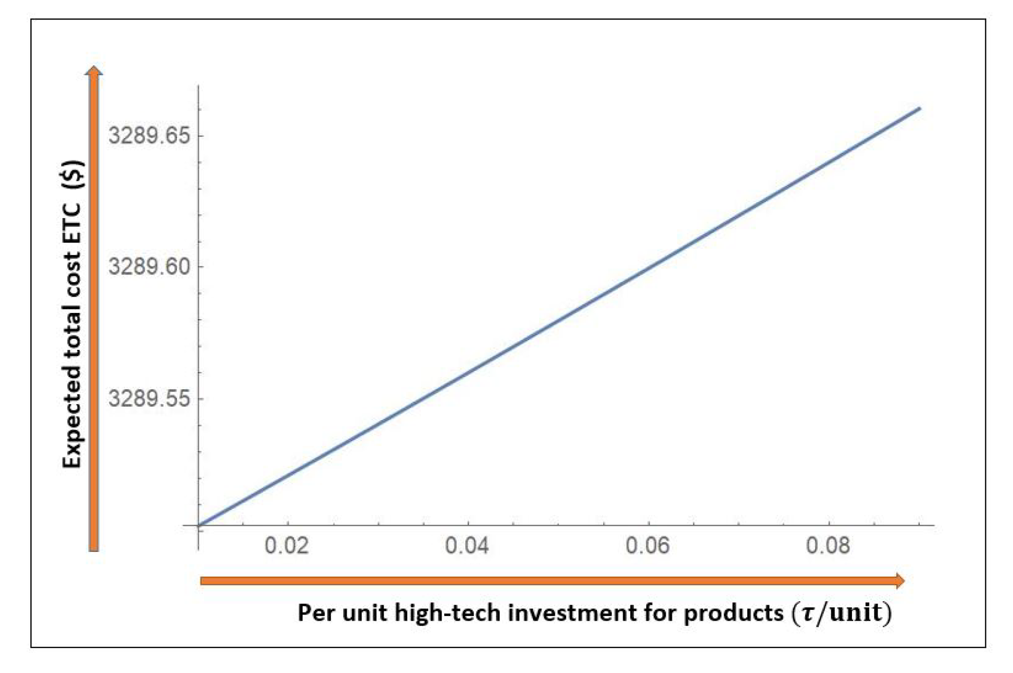
Due to the stochastic nature of breakdowns and repair times, the study extended the production inventory model to an integrated smart production maintenance model. The study infers the importance of performance quality parameter $\zeta$ for per-unit technological investment for products $\tau$, as even a 10% increase in $\zeta$ gives infeasible results for the proposed unreliable production model.

The manufacturing reliability depends on the system failure rate, and the system reliability is considered a decision variable. To increase the manufacturing reliability, an investment in smart production technology is made which based on raw material yield loss cost, manufacturing yield loss cost, tool/die cost for manufacturing machinery, per unit smart production cost based on reliability, and controllable production rates. As the time to failure and time to repair follows exponential distributions, the cycle length is a random parameter, so an abort/resume policy is considered. The mathematical problem was solved through Kuhn–Tucker considering reliability and productivity constraints. The model shows the practical implications of unreliable manufacturing system for industrial managers. Based on random failure rate and random repair rate, the managers get the information for optimal production quantity and optimal production rate. A more practical consideration is the variable demand which depends on the technology investment, as with the technology revolution, demand for high-tech products is increasing as compared to conventional consumer products; for this reason, the model provides better insight into investment in products as well as smart production technology. Some future extensions could be the consideration of automation policies for manufacturing systems. Also, the study does not consider the energy costs and carbon emissions associated with investments in new technology, which could be a genuine limitation of this research. Energy costs are considered as the biggest cost component in the production for complex and highly automated production systems. Asghar et al. [6] showed that energy consumption for an unreliable production system is a variable factor for different production states and specific energy consumption costs for an automated flexible production system can be reduced with improved manufacturing reliability. The study can be further extended to the concept [34] of imperfect production process for an unreliable manufacturing system as the production of defectives is an inevitable phenomena. Furthermore, considerations of deteriorating products is also an important extension of this work, and a good study in this direction is performed by [68]. One should consider that raw material and finished product deterioration is a more realistic but difficult issue, as the majority of production materials faces deterioration due to handling, storage, and lifetime limitations. Including carbon emissions cost in the production system is yet another extension of this paper, and to make the manufacturing process green and clean, such a study is done by [71]. This way one can analyze the economic and environmental implications of high-tech investment in manufacturing policies and product innovations. Another important and more current field of technological advancements that should be considered is modern e-commerce business practices for variable product demands. In this regard, the works of [72,73] provide a better understanding for offline and online business strategies.

References

- Kang, C.W.; Ramzan, M.B.; Sarkar, B.; Imran, M. Effect of inspection performance in smart manufacturing system based on human quality control system. Int. J. Adv. Manuf. Technol. 2018, 94, 4351–4364. [Google Scholar] [CrossRef]
- Sarkar, M.; Sarkar, B. Optimization of safety stock under controllable production rate and energy consumption in an automated smart production management. Energies 2019, 12, 2059. [Google Scholar] [CrossRef]
- Sarkar, M.; Sarkar, B.; Iqbal, M. Effect of energy and failure rate in a multi-item smart production system. Energies 2018, 11, 2958. [Google Scholar] [CrossRef]
- Wu, S.D.; Erkoc, M.; Karabuk, S. Managing capacity in the high-tech industry: A review of literature. Eng. Econ. 2005, 50, 125–158. [Google Scholar] [CrossRef]
- Chakraborty, T.; Giri, B.C.; Chaudhuri, K. Production lot sizing with process deterioration and machine breakdown. Eur. J. Oper. Res. 2008, 185, 606–618. [Google Scholar] [CrossRef]
- Asghar, I.; Sarkar, B.; Kim, S.j. Economic Analysis of an Integrated Production–Inventory System under Stochastic Production Capacity and Energy Consumption. Energies 2019, 12, 3179. [Google Scholar] [CrossRef]
- Marchi, B.; Zanoni, S.; Jaber, M.Y. Economic production quantity model with learning in production, quality, reliability and energy efficiency. Comput. Ind. Eng. 2019, 129, 502–511. [Google Scholar] [CrossRef]
- Lopes, R. Integrated model of quality inspection, preventive maintenance and buffer stock in an imperfect production system. Comput. Ind. Eng. 2018, 126, 650–656. [Google Scholar] [CrossRef]
- Marchi, B.; Zanoni, S.; Zavanella, L.; Jaber, M. Supply chain models with greenhouse gases emissions, energy usage, imperfect process under different coordination decisions. Int. J. Prod. Econ. 2019, 211, 145–153. [Google Scholar] [CrossRef]
- Chakraborty, T.; Giri, B.; Chaudhuri, K. Production lot sizing with process deterioration and machine breakdown under inspection schedule. Omega 2009, 37, 257–271. [Google Scholar] [CrossRef]
- Kang, K.; Subramaniam, V. Joint control of dynamic maintenance and production in a failure-prone manufacturing system subjected to deterioration. Comput. Ind. Eng. 2018, 119, 309–320. [Google Scholar] [CrossRef]
- Bhunia, A.K.; Shaikh, A.A.; Cárdenas-Barrón, L.E. A partially integrated production-inventory model with interval valued inventory costs, variable demand and flexible reliability. Appl. Soft Comput. 2017, 55, 491–502. [Google Scholar] [CrossRef]
- Ouaret, S.; Kenné, J.P.; Gharbi, A. Production and replacement policies for a deteriorating manufacturing system under random demand and quality. Eur. J. Oper. Res. 2018, 264, 623–636. [Google Scholar] [CrossRef]
- Bag, S.; Chakraborty, D.; Roy, A. A production inventory model with fuzzy random demand and with flexibility and reliability considerations. Comput. Ind. Eng. 2009, 56, 411–416. [Google Scholar] [CrossRef]
- AlDurgam, M.; Adegbola, K.; Glock, C.H. A single-vendor single-manufacturer integrated inventory model with stochastic demand and variable production rate. Int. J. Prod. Econ. 2017, 191, 335–350. [Google Scholar] [CrossRef]
- Ouaret, S.; Kenné, J.P.; Gharbi, A. Joint production and replacement planning for an unreliable manufacturing system subject to random demand and quality. IFAC-PapersOnLine 2018, 51, 951–956. [Google Scholar] [CrossRef]
- Manna, A.K.; Dey, J.K.; Mondal, S.K. Imperfect production inventory model with production rate dependent defective rate and advertisement dependent demand. Comput. Ind. Eng. 2017, 104, 9–22. [Google Scholar] [CrossRef]
- Zhu, X.; Jiao, C.; Yuan, T. Optimal decisions on product reliability, sales and promotion under nonrenewable warranties. Reliab. Eng. Syst. Saf. 2018, 192, 106268. [Google Scholar] [CrossRef]
- Shah, N.H.; Vaghela, C.R. Imperfect production inventory model for time and effort dependent demand under inflation and maximum reliability. Int. J. Syst. Sci. Oper. Logist. 2018, 5, 60–68. [Google Scholar] [CrossRef]
- Khara, B.; Dey, J.K.; Mondal, S.K. An inventory model under development cost-dependent imperfect production and reliability-dependent demand. J. Manag. Anal. 2017, 4, 258–275. [Google Scholar] [CrossRef]
- Shah, N.H.; Naik, M.K. Inventory Policies with Development Cost for Imperfect Production and Price-Stock Reliability-Dependent Demand. In Optimization and Inventory Management; Springer: Singapore, 2020; pp. 119–136. [Google Scholar]
- Çanakoğlu, E.; Bilgic, T. Analysis of a two-stage telecommunication supply chain with technology dependent demand. Eur. J. Oper. Res. 2007, 177, 995–1012. [Google Scholar] [CrossRef]
- Rosenblatt, M.J.; Lee, H.L. Economic production cycles with imperfect production processes. IIE Trans. 1986, 18, 48–55. [Google Scholar] [CrossRef]
- Porteus, E.L. Optimal lot sizing, process quality improvement and setup cost reduction. Oper. Res. 1986, 34, 137–144. [Google Scholar] [CrossRef]
- Kim, C.H.; Hong, Y. An optimal production run length in deteriorating production processes. Int. J. Prod. Econ. 1999, 58, 183–189. [Google Scholar]
- Akella, R.; Kumar, P. Optimal control of production rate in a failure prone manufacturing system. IEEE Trans. Autom. Control 1986, 31, 116–126. [Google Scholar] [CrossRef]
- Sharifnia, A. Production control of a manufacturing system with multiple machine states. IEEE Trans. Autom. Control 1988, 33, 620–625. [Google Scholar] [CrossRef]
- Posner, M.; Berg, M. Analysis of a production-inventory system with unreliable production facility. Oper. Res. Lett. 1989, 8, 339–345. [Google Scholar] [CrossRef]
- Boukas, E.K.; Haurie, A. Manufacturing flow control and preventing maintenance: A stochastic control approach. IEEE Trans. Autom. Control 1990, 35, 1024–1031. [Google Scholar] [CrossRef]
- Groenevelt, H.; Pintelon, L.; Seidmann, A. Production batching with machine breakdowns and safety stocks. Oper. Res. 1992, 40, 959–971. [Google Scholar] [CrossRef]
- Groenevelt, H.; Pintelon, L.; Seidmann, A. Production lot sizing with machine breakdowns. Manag. Sci. 1992, 38, 104–123. [Google Scholar] [CrossRef]
- Nodem, F.D.; Kenné, J.P.; Gharbi, A. Hierarchical decision making in production and repair/replacement planning with imperfect repairs under uncertainties. Eur. J. Oper. Res. 2009, 198, 173–189. [Google Scholar] [CrossRef]
- Sarkar, B.; Sana, S.S.; Chaudhuri, K. Optimal reliability, production lotsize and safety stock: An economic manufacturing quantity model. Int. J. Manag. Sci. Eng. Manag. 2010, 5, 192–202. [Google Scholar] [CrossRef]
- Sarkar, B.; Sana, S.S.; Chaudhuri, K. Optimal reliability, production lot size and safety stock in an imperfect production system. Int. J. Math. Oper. Res. 2010, 2, 467–490. [Google Scholar] [CrossRef]
- Bhuniya, S.; Sarkar, B.; Pareek, S. Multi-Product Production System with the Reduced Failure Rate and the Optimum Energy Consumption under Variable Demand. Mathematics 2019, 7, 465. [Google Scholar] [CrossRef]
- Glock, C.H. Batch sizing with controllable production rates. Int. J. Prod. Res. 2010, 48, 5925–5942. [Google Scholar] [CrossRef]
- Glock, C.H. Batch sizing with controllable production rates. Int. J. Prod. Res. 2011, 49, 2455. [Google Scholar] [CrossRef][Green Version]
- Shepherd, R.W. Theory of Cost and Production Functions; Princeton University Press: Princeton, NJ, USA, 2015. [Google Scholar]
- Sarkar, B.; Majumder, A.; Sarkar, M.; Kim, N.; Ullah, M. Effects of variable production rate on quality of products in a single-vendor multi-buyer supply chain management. Int. J. Adv. Manuf. Technol. 2018, 99, 567–581. [Google Scholar] [CrossRef]
- Khouja, M.; Mehrez, A. Economic production lot size model with variable production rate and imperfect quality. J. Oper. Res. Soc. 1994, 45, 1405–1417. [Google Scholar] [CrossRef]
- Rishel, R. Control of systems with jump Markov disturbances. IEEE Trans. Autom. Control 1975, 20, 241–244. [Google Scholar] [CrossRef]
- Olsder, G.; Suri, R. Time-optimal control of parts-routing in a manufacturing system with failure-prone machines. In Proceedings of the 1980 19th IEEE Conference on Decision and Control including the Symposium on Adaptive Processes, Albuquerque, NM, USA, 10–12 December 1980; pp. 722–727. [Google Scholar]
- Deb, M.; Chaudhuri, K. An EOQ model for items with finite rate of production and variable rate of deterioration. Opsearch 1986, 23, 175–181. [Google Scholar]
- Mandal, B.a.; Phaujdar, S. An inventory model for deteriorating items and stock-dependent consumption rate. J. Oper. Res. Soc. 1989, 40, 483–488. [Google Scholar] [CrossRef]
- Bhunia, A.; Maiti, M. Deterministic inventory model for deteriorating items with finite rate of replenishment dependent on inventory level. Comput. Oper. Res. 1998, 25, 997–1006. [Google Scholar] [CrossRef]
- Abad, P.L. Optimal lot size for a perishable good under conditions of finite production and partial backordering and lost sale. Comput. Ind. Eng. 2000, 38, 457–465. [Google Scholar] [CrossRef]
- Giri, B.C.; Yun, W.; Dohi, T. Optimal design of unreliable production–inventory systems with variable production rate. Eur. J. Oper. Res. 2005, 162, 372–386. [Google Scholar] [CrossRef]
- Larsen, C. The economic production lot size model extended to include more than one production rate. Int. Trans. Oper. Res. 2005, 12, 339–353. [Google Scholar] [CrossRef]
- AlDurgam, M.M.; Duffuaa, S.O. Optimal joint maintenance and operation policies to maximise overall systems effectiveness. Int. J. Prod. Res. 2013, 51, 1319–1330. [Google Scholar] [CrossRef]
- Sarkar, M.; Hur, S.; Sarkar, B. Effects of Variable Production Rate and Time-Dependent Holding Cost for Complementary Products in Supply Chain Model. Math. Probl. Eng. 2017. [Google Scholar] [CrossRef]
- Alfares, H.K.; Ghaithan, A.M. EOQ and EPQ Production-Inventory Models with Variable Holding Cost: State-of-the-Art Review. Arab. J. Sci. Eng. 2019, 44, 1737–1755. [Google Scholar] [CrossRef]
- Dey, B.K.; Sarkar, B.; Pareek, S. A Two-Echelon Supply Chain Management With Setup Time and Cost Reduction, Quality Improvement and Variable Production Rate. Mathematics 2019, 7, 328. [Google Scholar] [CrossRef]
- Bhandari, R.; Sharma, P. The economic production lot-size model with variable cost function. Opsearch 1999, 36, 137–150. [Google Scholar] [CrossRef]
- Khalifehzadeh, S.; Fakhrzad, M. A Modified Firefly Algorithm for optimizing a multi stage supply chain network with stochastic demand and fuzzy production capacity. Comput. Ind. Eng. 2019, 133, 42–56. [Google Scholar] [CrossRef]
- Harris, F.W. Operations and cost. In Factory Management Series; AW Shaw Co.: Chicago, IL, USA, 1915; pp. 48–52. [Google Scholar]
- Wilson, R. A Scientific Routine for Stock Control; Harvard Univ.: Cambridge, MA, USA, 1934. [Google Scholar]
- Cho, D.I. Analysis of optimal production and advertising policies. Int. J. Syst. Sci. 1996, 27, 1297–1305. [Google Scholar] [CrossRef]
- Hazari, S.; Maity, K.; Dey, J.K.; Kar, S. Advertisement policy and reliability dependent imperfect production inventory control problem in bi–fuzzy environment. Int. J. Oper. Res. 2015, 22, 342–365. [Google Scholar] [CrossRef]
- Rivera-Gómez, H.; Gharbi, A.; Kenné, J.P.; Montano-Arango, O.; Hernandez-Gress, E.S. Production control problem integrating overhaul and subcontracting strategies for a quality deteriorating manufacturing system. Int. J. Prod. Econ. 2016, 171, 134–150. [Google Scholar] [CrossRef]
- Yin, K.K.; Liu, H.; Yin, G.G. Stochastic models and numerical solutions for production planning with applications to the paper industry. Comput. Chem. Eng. 2003, 27, 1693–1706. [Google Scholar] [CrossRef]
- Yang, P.; Wee, H.M.; Hsu, P. Collaborative vendor–buyer inventory system with declining market. Comput. Ind. Eng. 2008, 54, 128–139. [Google Scholar] [CrossRef]
- Goyal, M.; Netessine, S. Strategic technology choice and capacity investment under demand uncertainty. Manag. Sci. 2007, 53, 192–207. [Google Scholar] [CrossRef]
- Yuan, X.; Shen, L.; Ashayeri, J. Dynamic simulation assessment of collaboration strategies to manage demand gap in high-tech product diffusion. Robot. Comput.-Integr. Manuf. 2010, 26, 647–657. [Google Scholar] [CrossRef]
- Sana, S.; Chaudhuri, K.; Mahavidyalaya, B. On a volume flexible production policy for a deteriorating item with time-dependent demand and shortages. Adv. Model. Optim. 2004, 6, 57–74. [Google Scholar]
- Ross, S.M. Introduction to Probability Models; Academic Press: Cambridge, MA, USA, 2014. [Google Scholar]
- Goyal, S.; Giri, B.C. The production–inventory problem of a product with time varying demand, production and deterioration rates. Eur. J. Oper. Res. 2003, 147, 549–557. [Google Scholar] [CrossRef]
- Malik, A.I.; Kim, B.S. A Constrained Production System Involving Production Flexibility and Carbon Emissions. Mathematics 2020, 8, 275. [Google Scholar] [CrossRef]
- Ullah, M.; Sarkar, B.; Asghar, I. Effects of Preservation Technology Investment on Waste Generation in a Two-Echelon Supply Chain Model. Mathematics 2019, 7, 189. [Google Scholar] [CrossRef]
- Ullah, M.; Sarkar, B. Recovery-channel selection in a hybrid manufacturing-remanufacturing production model with RFID and product quality. Int. J. Prod. Econ. 2020, 219, 360–374. [Google Scholar] [CrossRef]
- Sarkar, B.; Guchhait, R.; Sarkar, M.; Cárdenas-Barrón, L.E. How does an industry manage the optimum cash flow within a smart production system with the carbon footprint and carbon emission under logistics framework? Int. J. Prod. Econ. 2019, 213, 243–257. [Google Scholar] [CrossRef]
- Sarkar, B.; Ullah, M.; Kim, N. Environmental and economic assessment of closed-loop supply chain with remanufacturing and returnable transport items. Comput. Ind. Eng. 2017, 111, 148–163. [Google Scholar] [CrossRef]
- Sarkar, B.; Ullah, M.; Choi, S.B. Joint inventory and pricing policy for an online to offline closed-loop supply chain model with random defective rate and returnable transport items. Mathematics 2019, 7, 497. [Google Scholar] [CrossRef]
- Sarkar, B.; Tayyab, M.; Choi, S.B. Product Channeling in an O2O supply chain management as power transmission in electric power distribution systems. Mathematics 2019, 7, 4. [Google Scholar] [CrossRef]