Article

Evaluation of the Mass Diffusion Coefficient and Mass Biot Number Using a Nondominated Sorting Genetic Algorithm

by
Radosław Winiczenko
*,
Krzysztof Górnicki
and
Agnieszka Kaleta
Institute of Mechanical Engineering, Warsaw University of Life Sciences, Nowoursynowska 164 St., 02-787 Warsaw, Poland
*
Author to whom correspondence should be addressed.
Symmetry 2020, 12(2), 260; https://doi.org/10.3390/sym12020260
Submission received: 22 January 2020 / Revised: 4 February 2020 / Accepted: 6 February 2020 / Published: 8 February 2020

Abstract

:
A precise determination of the mass diffusion coefficient and the mass Biot number is indispensable for deeper mass transfer analysis that can enable finding optimum conditions for conducting a considered process. The aim of the article is to estimate the mass diffusion coefficient and the mass Biot number by applying nondominated sorting genetic algorithm (NSGA) II genetic algorithms. The method is used in drying. The maximization of coefficient of correlation (R) and simultaneous minimization of mean absolute error (MAE) and root mean square error (RMSE) between the model and experimental data were taken into account. The Biot number and moisture diffusion coefficient can be determined using the following equations: Bi = 0.7647141 + 10.1689977s − 0.003400086T + 948.715758s2 + 0.000024316T2 − 0.12478256sT, D = 1.27547936∙10−7 − 2.3808∙10−5s − 5.08365633∙10−9T + 0.0030005179s2 + 4.266495∙10−11T2 + 8.33633∙10−7sT or Bi = 0.764714 + 10.1689091s − 0.003400089T + 948.715738s2 + 0.000024316T2 − 0.12478252sT, D = 1.27547948∙10−7 − 2.3806∙10−5s − 5.08365753∙10−9T + 0.0030005175s2 + 4.266493∙10−11T2 + 8.336334∙10−7sT. The results of statistical analysis for the Biot number and moisture diffusion coefficient equations were as follows: R = 0.9905672, MAE = 0.0406375, RMSE = 0.050252 and R = 0.9905611, MAE = 0.0406403 and RMSE = 0.050273, respectively.

1. Introduction

The diffusion coefficient (D) is an important mass exchange parameter. The values of this property are needed in the mathematical description of various processes. The discussed coefficient is affected by intermolecular interaction and depends on solution concentration and kind of substances [1]. The diffusivity of such substances in food as water, salt, small organic acids or aromas is determined in the literature [2]. Gross and Ruegg [3] measured the diffusion coefficient of salt and aroma in gels and salt in cheese. Whereas Warin et al. [4] determined the diffusivity of disaccharides in a two-phase medium composed of a milk product with a fruit layer in its bottom. Rattanakijsuntorn et al. [5] developed the technique of measurement of the drugs diffusion coefficient in the vitreous humor using Finite Element Method (FEM) and Magnetic Resonance Imaging (MRI). The method can be applied to different types of bioporous media.
The diffusion of liquid, gases and vapors in heterogeneous and non-isotropic media depends very often on the direction of mass transfer and; therefore, the diffusivity value varies along the diffusion path [6]. In some cases, the solid can be deformed by the influence of concentration gradients. Moreover, the interaction between solid and diffusing substances can occur. Mentioned processes influence diffusion and; therefore, the diffusion in solid materials is described using an effective diffusion coefficient [1]. Zamel et al. [7] determined such a coefficient in the carbon paper gas-diffusion layer (GDL) used in polymer electrolyte membrane (PEM) fuel cells, whereas Chan et al. [8] measured the discussed coefficient through PEM fuel call GDLs with and without the microporous layer. Garcia-Salaberri et al. [9] determined the effective gas-diffusion coefficient for dry and partially-saturated carbon paper gas-diffusion layers. Wang et al. [10] studied the impact of humic acid on fouling problems in the application of membrane technology for drinking water treatments and examined the effects of calcium and pH on the effective diffusion coefficient of humic acid. Stewart [11] reviewed the discussed diffusion property in biofilms.
Data concerning diffusion properties of solids with respect to moisture are important, among others, in such fields of application as building materials, drying and rehydration.
Global warming causes a growing interest not only in renewable materials but in energy savings in building construction as well [12]. Therefore the study of mass and heat exchange in building materials is needed [13]. The value of the moisture diffusion coefficient is necessary to solve the mass transfer equation. The discussed coefficient was determined, among others, for low- and medium-density fiberboard, spruce wood oriented in tangential and radial directions [12] and northern red oak (Quercus rubra) [14].
Fick’s second law of diffusion can be applied for explaining and/or modelling the moisture movement during solid body drying. Knowledge of the values of the moisture diffusion coefficient is necessary for solving the Fickian equation. The mechanism of drying of hygroscopic-porous products is very complicated. It can be accepted that moisture is transported by water, vapor and Knudsen diffusion, by hydrodynamic and capillary flow, and also by condensation effects. There is a mixture of above mentioned types of moisture movement very often, and their contributions to the total moisture transport depend on the place in the dried solid and time of drying. For this reason, the moisture diffusion coefficient in the Fickian equation is called the effective coefficient because it takes into account the total moisture transport [15,16]. The discussed coefficient depends on temperature [17,18], on the moisture content [19,20,21] and the material structure [2]. Effective diffusivity of moisture was determined, among others, for: Willow (Salix viminalis) stems dried by natural wind [22], pumpkin (Cucurbita maxima) dried in vacuum dryer [23], air-dried date palm (Phoenix dactylifera L.) fruits [24], mushrooms dried in a hybrid-solar dryer [25], and apples (var. Ligol) dried in a fluidized dryer [26].
Rehydration is a complicated mass transport process. Liquid imbibition in the porous body, such as dried products, is governed by complex phenomena including hydraulic and capillary flow, convection and molecular diffusion. To predict liquid absorption during rehydration, Fick’s second law of diffusion is often applied. Fickian equation for rehydration contains the effective diffusion coefficient, an apparent property that takes into account all the factors involved in the process [27]. The effective diffusivity depends on temperature, moisture content and material structure [24,28,29,30]. The discussed property was determined, among others, for the process of water absorption by amaranth grain in the process of soaking [31]. Cunningham et al. [32] investigated the influence of drying method, temperature and pre-drying treatments on the moisture diffusion coefficient during rehydration of dried potatoes. Whereas Maldonado et al. [33] determined the effect of processing conditions on water diffusion in dried mangoes during rehydration. Ramallo and Albani [34] determined the effective water diffusion coefficient in a packaged yerba mate.
To solve the Fickian equation, appropriate initial and boundary conditions have to be adopted. Mass transport at the surface of the porous body can be described using boundary condition of the first kind or the third kind [35]. Condition of the first kind informs that the external resistance to mass movement can be treated as negligible, whereas the discussed condition of the third kind indicates that the mass flux from the porous object surface is represented in the form of diffusing component concentration difference between the surface and the equilibrium concentration.
In the case when the third kind condition is expressed in the dimensionless form, the dimensionless Biot number (Bi) appeared in a partial differential equation. Bi (Bi = kL/D) represents the interdependence between internal and external mass fluxes and; therefore, informs about the controlling mechanism of mass exchange in the process [17,20,36]. For Bi < 0.1 the surface mass resistance in the boundary layer of external fluid is bigger than the internal resistance of the mass diffusion in porous material [36]. Bi > 100 [36] or even Bi > 40 [21] informs that the internal resistance of mass diffusion controls mass exchange. The third kind of boundary condition for moisture transport during drying was applied, among others, by Miketinac et al. [37] for grain, Wang and Brennan [38] for potato, Białobrzewski [39] for celery root and Górnicki and Kaleta [40] for blanched carrot cubes. Mass Biot number was determined in several publications to achieve a deeper insight into such investigated processes as drying of shrinking potato slabs [17], heat and mass transport during porous object drying [41], air drying of small wet porous materials [42] or apple-leather and wheat drying [20]. Zielińska and Markowski [19] analyzed the changes in Bi vs. time and temperature during drying of carrot cubes in a spout-fluidized bed dryer.
Many works have been dedicated to data modelling by an artificial neural network. Artificial neural networks (ANNs) are comprised of neurons with associated weights and activation functions. These neurons are simplified computational models based on our understanding of biological neurons. The weights represent the relationship between the neurons. Various architectures, including feed-forward neural networks, with associated learning schemes, such as back-propagation, have been proposed using networks of these neurons. The combination of feed-forward networks and fuzzy decision rules allowed for the creation of the adaptive neuro-fuzzy inference system (ANFIS). The ANFIS is a method used for finding nonlinear function. The data are used to train by gradient descent and least-squares methods. More details of this combination of systems can be found in [43].
Recently, many research and technical papers have been dealing with optimization issues. It can be seen that soft computing is realized through techniques such as response surface methodology and genetic algorithms. Response surface methodology (RSM) is a statistical method often used for planning experiments, modelling and optimization. This method allows one to efficiently find the relationship between inputs and outputs parameters. The relationships between them are described by quadratic functions that are then optimized. In this way, it reduces the time and costs of the experiment. Examples of optimization tasks using RSM can be found in [44,45].
Genetic algorithms (GAs) are an efficient optimization technique. This method is often used for global optimization. GAs in comparison with the RSM method can be an efficient tool for solving tasks which do not need to be differentiable. Moreover, GAs are often used to find the optimum for discontinuous or multimodal functions [46]. The authors chose GA because performs better than RSM when a large number of experiments are affordable. Response surface methods are used in small spaces to search within established boundaries.
Recently, various papers related to multi-objective optimization (MOO) have been published. MOO has been also realized in the food industry. Kopsidas [47] proposed a multi-objective optimization for the process design of a table olive preparation system. Kiranoudis and Markatos [48] used non-preference multi-criteria optimization methods to drying of sliced potato. Therdthai et al. [49] developed the mathematical models to describe the effect of the baking temperature profile and baking time on the weight loss, crust colour and internal temperature for white sandwich bread. Erdogdu and Balaban [50] applied a nonlinearly constrained optimization method to two different shapes, subjected to the same thermal processing boundary conditions, to find a variable process temperature profile to maximize the average retention volume of thiamine. MOO has been realized in wine filtration [51]. Hadiyanto et al. [52] sequentially applied a multi-objective optimization to improve the product range of baking systems. Further applications of MOO to simulated moving beds in food processing are shown in [53,54,55]. Abakarov et al. [56] have used a multi-objective optimization technique for the thermal sterilization of packaged foods. The quality indicators of apple issues for drying and rehydrated processes using a non-sorting genetic algorithm (NSGA) were described in [57,58].
MOO applications in the food industry concentrate on finding Pareto optimal solutions for product quality and cost objectives, with many of them using MOO methods which generate multiple solutions. Such methods are readily available and effective at generating Pareto optimal solutions, as reported Seng and Rangaiah [59].
A precise evaluation of the mass diffusion coefficient and the mass Biot number is indispensable for deeper mass transfer analysis that can enable to find optimum conditions for conducting a considered process.
As mentioned, some authors have described the mass diffusion coefficient and the mass Biot number. Górnicki et al. [60] estimated the mass Biot number using GA. Authors presented the method of Biot number estimation in the drying process and proposed equations for determination of Bi. The mass Biot number depended on the drying temperature in the proposed equations. Therefore in the current paper, the authors decided to estimate, additionally, the mass diffusion coefficient using NSGA II. The method is used in the drying process. The equations for the mass diffusion coefficient and the mass Biot number determination will be proposed. The purpose of the work is also to make D and Bi dependent not only on the drying temperature but also on the characteristic dimension of the dried sample as a novelty. These equations will be more widely used in the application.

2. Materials and Methods

2.1. Material

The parsley roots of Berlińska variety were cut into 3, 6 and 9 mm thick slices. The research material was dried in natural convection conditions. The drying air temperatures were the following: 40, 50, 60 and 70 °C.
The detail about the equipment, measurements and their accuracy have been described in [61].

2.2. Moisture Transfer Analysis

It is assumed very often that the water transfer inside the dried solid is only a diffusion movement in the convection drying of materials with high initial moisture content. Therefore the equation used for the description of the drying process (for an infinite plane (slices)) takes the following form [62,63,64]:
M t = D 2 M x 2 ( t > 0 ; s < x < s )
The following simplifications were used in this equation: The volume and shape of the drying sample do not change during drying, D is constant.
Initial and boundary conditions are taken for solving Equation (1) were as follows [62,64]:
  • Initial condition: M at any point of the sample is the same at the beginning of drying:
M ( x , 0 ) = M 0 = const ,
  • Boundary conditions of the third kind: The moisture flux from the surface of the sample is described in terms of moisture content difference between the surface and the equilibrium moisture content:
± D M ( ± s , t ) x = k [ M ( ± s , t ) M e ] ,
An analytical solution of Equation (1) with the initial condition (Equation (2)) and boundary conditions (Equation (3)) in the form of mean moisture content being a function of time can be expressed as [62,64]:
M R = M M e M 0 M e = i = 1 B i exp [ μ i 2 D s 2 t ] ,
where:
B i = 2 Bi 2 μ i 2 ( Bi 2 + Bi + μ i 2 ) ,   ctg μ i = 1 Bi μ i
A method of solving the diffusion equation for different geometries can be found in the literature [62,64].
The Biot number in Equation (5) and D in Equation (4) were assumed dependent on temperature and characteristic dimension using the formulas:
Bi = a B i + b B i s + c B i T + d B i s 2 + e B i T 2 + f B i s T ,
D = a D + b D s + c D T + d D s 2 + e D T 2 + f D s T ,
A similar type of dependents (linear, logarithmic, exponential, rational, square type of equations) were considered in the literature. The authors investigated the effects of the particle shape, particle size, initial material load [65], initial height of the layer, drying air temperature, air velocity [66] and vegetable species [67] on the drying models coefficients and constants.
To compare the fit quality of the model (4) to experimental data, the root mean square error (RMSE), the mean absolute error (MAE) and the coefficient of correlation (R) were taken (the most commonly used [60,67]):
RMSE = 1 N i = 1 N ( M R pred M R e x p ) 2 ,
MAE = 1 N i = 1 N | M R pred M R e x p | ,
R 2 = 1 i = 1 N ( M R pred M R e x p ) 2 i = 1 N ( M R pred M R ¯ e x p ) 2

2.3. Multi-Objective Optimization

In many applications, the cost function has multiple, oftentimes conflicting, objectives. This will be a multi-objective optimization problem (MOO) problem. In multi-objective optimization, usually, no single solution exists that is optimum with respect to all objectives. Therefore a set of optimal solutions are obtained, often known as Pareto optimal solutions or noninferior solutions, and all these solutions are equally satisfactory.
The aim of multi-objective optimization is finding as many of these solutions as possible. If the reallocation of resources cannot improve one cost without raising another cost, then the solution is Pareto optimal. Pareto solution returns a population with many members on the Pareto front. The population is ordered based on dominance. Solution S1 dominates solution S2 if S1 has a lower cost than S2 for at least one of the objective functions and is not worse with respect to the remaining objective functions.
A noninferior solution is optimal if no other solution dominates that solution with respect to the cost functions. A solution is nondominated if no solution can be found that dominates it. Once this set of solutions is found, then the user can select a single solution based on various post-optimization trade-offs rather than weighing the costs. One way of finding the Pareto front is to run an algorithm for many various combinations of the fitness function weights. Each optimal solution is on the Pareto front. This approach needs too many runs to estimate the Pareto set. The multi-objective genetic algorithm (MOGA) starts by finding all nondominated chromosomes of a population and gives them a rank of one, as reported by Fonesca and Flemming [68].
Deb [69] proposed a new nondominated sorting genetic algorithm (NSGA) that uses several layers for the classification of individuals. Before selection, the population is ordered in terms of dominance. All nondominated individuals fall into one category. An artificial match value is introduced that is proportional to the population size. In this way, individuals are given equal reproductive potential. To maintain population diversity, this artificial fitness function is shared. Then the next group of nondominated individuals is classified. This process is repeated until all individuals in the population have been classified. A full description of the algorithm can be found in the literature [69].
The next NSGA II algorithm improves the NSGA algorithm by reducing the computational difficulty of the nondominated sorting, introducing elitism, replacing sharing with crowded comparison to reduce computations.
Figure 1 shows a flowchart of this Pareto genetic algorithm. This approach allows an easier way to trade off the infinite number of optimal solutions to the MOO problem. The Pareto genetic algorithm introduced here works with two fitness functions. It can be easily modified to work with more. A Pareto solution needs a large population size to work well since it is trying to define the Pareto front. Accordingly, we only include the tournament selection and mutation operator in the genetic algorithm. More details are described in the literature [69].

2.4. The Optimization Tasks

The optimization problem was divided into two tasks. The first one was the evaluation of the mass diffusion coefficient and Biot number from Equation (4) for each drying temperature: 40, 50, 60 and 70 °C and for each characteristic dimension (slices thickness): 3, 6 and 9 mm. The second optimization task was to determine the constants in Equations (6) and (7).
Both RMSE and MAE were minimized, whereas R was maximized, for the difference between the data and objective function for considered optimized tasks. The algorithm randomly selects a set of models by minimizing the error between the proposed model and experimental data. Next, it evolves them to give the best fit, hence the MOO problem was formulated in the following way:
Minimum = { Mininium RMSE Minimum MAE Maximum R
The optimization task was solved in MATLAB Optimization Toolbox™ using the following options: The “crossover” and “mutation” rates of 0.7 and 0.15, respectively; “ParetoFraction” of 0.5; number of generations of 600 multiplied by number of variables; “Population size” of 50 multiplied by number of variables; and “Tournament” method as selection function [70].

3. Results and Discussion

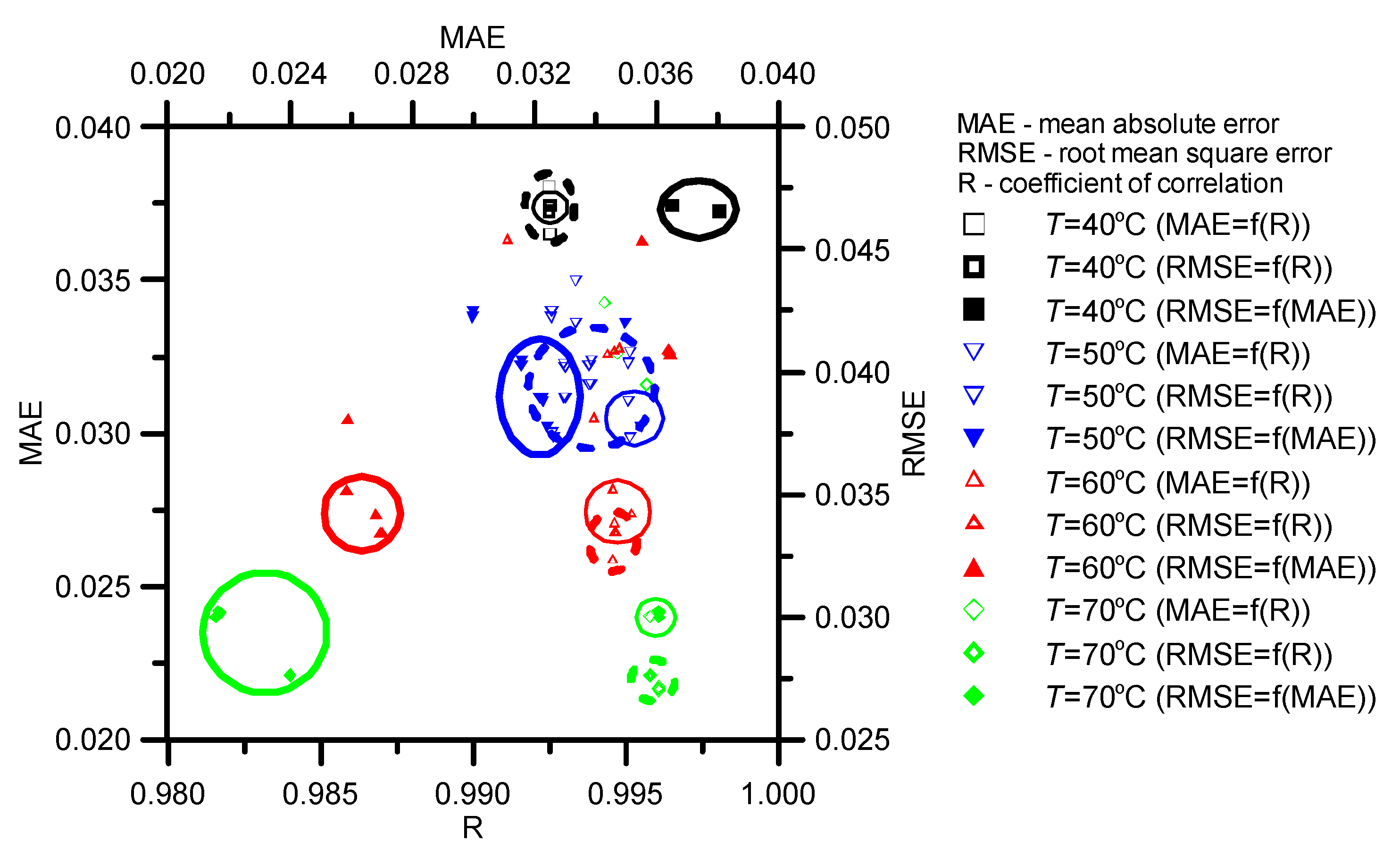
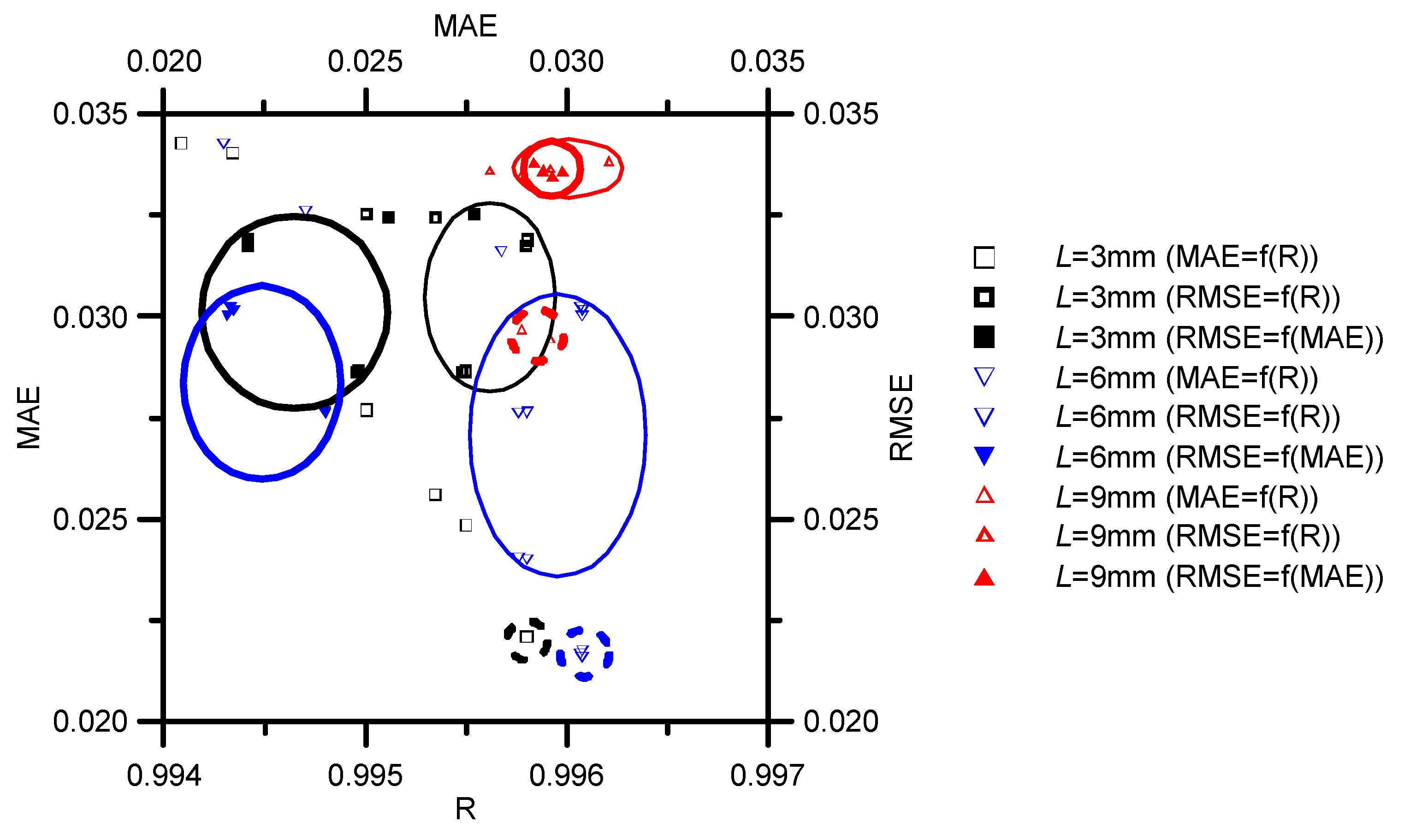
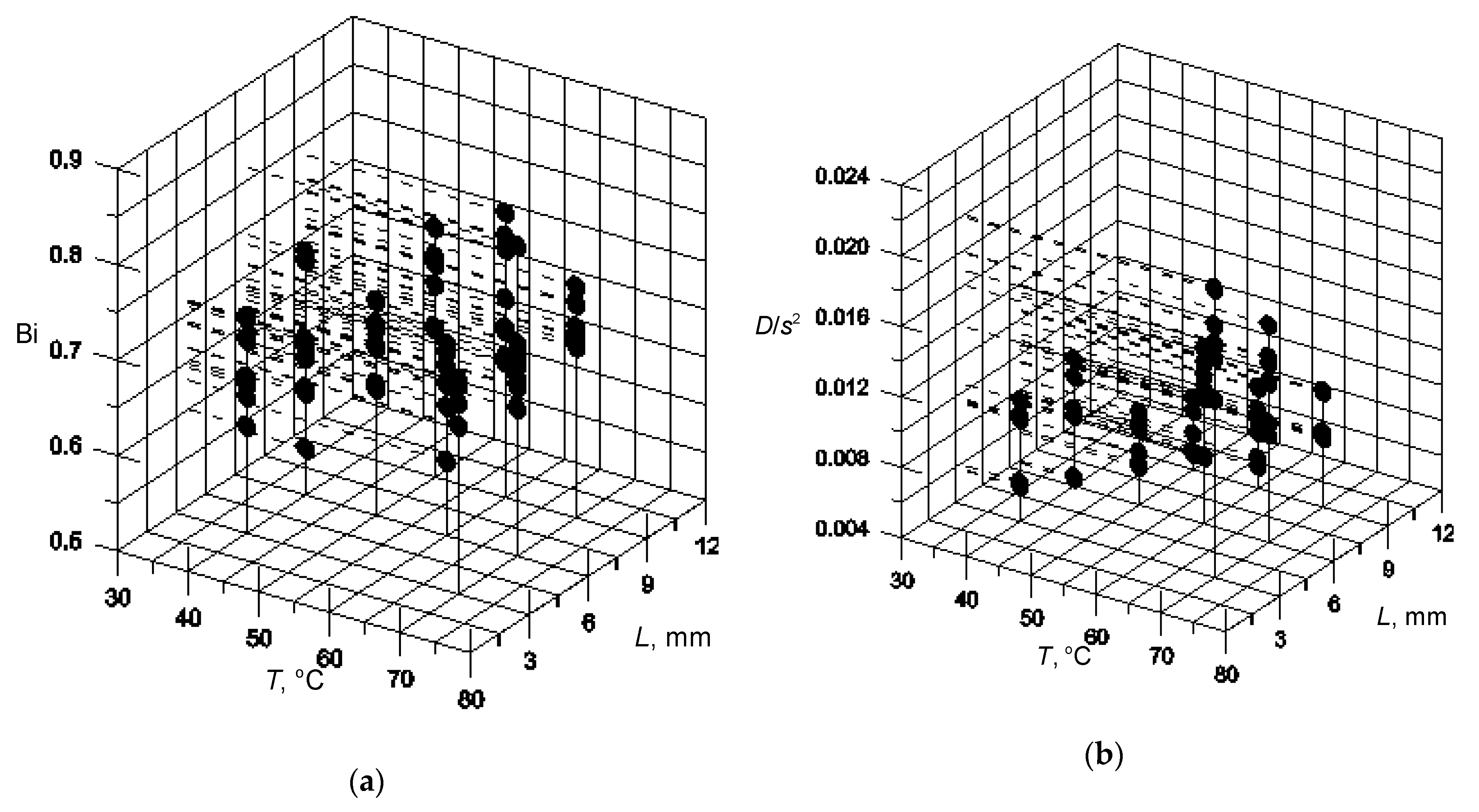
3.1. Optimization of Bi and D

The results of the optimization tasks described by Equations (4) and (11) are shown in Table S1 and the Figure 2, Figure 3 and Figure 4. The best solution for the optimization task in the case of drying at 40 °C for slices 3 mm thick, with the largest R for ID 40-3_5 (R = 0.9939), ID 40-3_8 (R = 0.9937) and ID 40-30_6 and ID 40-3_7 (R = 0.9935) for which Bi is 0.7264, 0.7243, 0.7016 and 0.7038, respectively. The RMSE values were characterized by the following ID 40-3_1 and ID 40-3_2 (RMSE = 0.4032), ID 40-3_4 (RMSE = 0436) and ID 40-3_8 (RMSE = 0.0447). The best solutions for the smallest MAE values are ID 40-3_9 (MAE = 0.0329), ID 40-3_3 (MAE = 0.340), ID 40-3_4 (MAE = 0.0351), ID 40-3_1 (MAE = 0.0353) and ID 40-3_2 (MAE = 0.0354). For the largest R and smallest RMSE, ID 40-3_8 can be used as the best solution, while the smallest RMSE and smallest MAE can be ID 40-3_1 and ID 40-3_4. However, in the case of a full optimization task (described by Equation (11)), it is difficult to give a one-factor solution. The R-value is in continuous conflict with RMSE and MAE values, which have higher values than for the best solutions (see, for example, ID 40-3_5-ID 40-3_7). The Pareto set of the best solutions for 40 °C indicates the greatest dispersion of solutions when the MAE and R criterion is considered (see Figure 2).
Bi calculated for drying at 50 °C shows the smallest RMSE = 0.0373 and the greatest R = 0.9951 for ID 50-6_3. The value of MAE = 0.0300 is the smallest for ID 50-6_1 and ID 50-6_4. The solution of R maximization is ID 50-6_9 (0.9951). From Table S1 it can be seen that the solutions are characterized by better statistics than for the temperature of 40 °C. The dispersion of the best solutions is larger compared with one for the higher temperatures (see Figure 2).
The drying at 60 °C indicates the smallest RMSE for ID 60-6_2 and ID 60-6_6 (0.0334). For ID 60-6_4, R is the greatest (0.9952). The result of MAE minimization is ID 60-6_1 and ID 60-6_3 (0.0259). The results for 60 °C are characterized by the smallest dispersion (see Figure 2).
The set of the best solutions for 70 °C shows the smallest RMSE = 0.0276 for ID 70-6_3 and ID 70-6_7. The result of MAE minimization is ID 70-6_4 (0.0216), with the solutions for ID 70-6_2 and ID 70-6_5 (0.0217, differences 0.0001).
It can be seen that the optimization solutions are characterized by better results (R, RMSE, MAE) for average drying temperatures (Figure 2). For T = 40 °C (R~0.993, RMSE~0.047, MAE~0.038), and T = 70 °C (R~0.996, RMSE~0.3 and MAE~0.022).
Statistics for Pareto optimal sets at T = 70 °C and various thicknesses are presented in Figure 3. The Biot number calculated for 6 mm slices, dried at 70 °C (ID = 70-6_4) has the best statistical values (see Table S1 and Figure 3). In this case, the smallest MAE = 0.0216 and the largest R = 0.9961 were obtained. The statistical results for the slices of 6 mm dried at T = 70 °C are larger than for the other thickness (see Figure 3). The Pareto set of the best solutions as for as the slices of 9 mm are considered shows the smallest dispersion (see Figure 3).

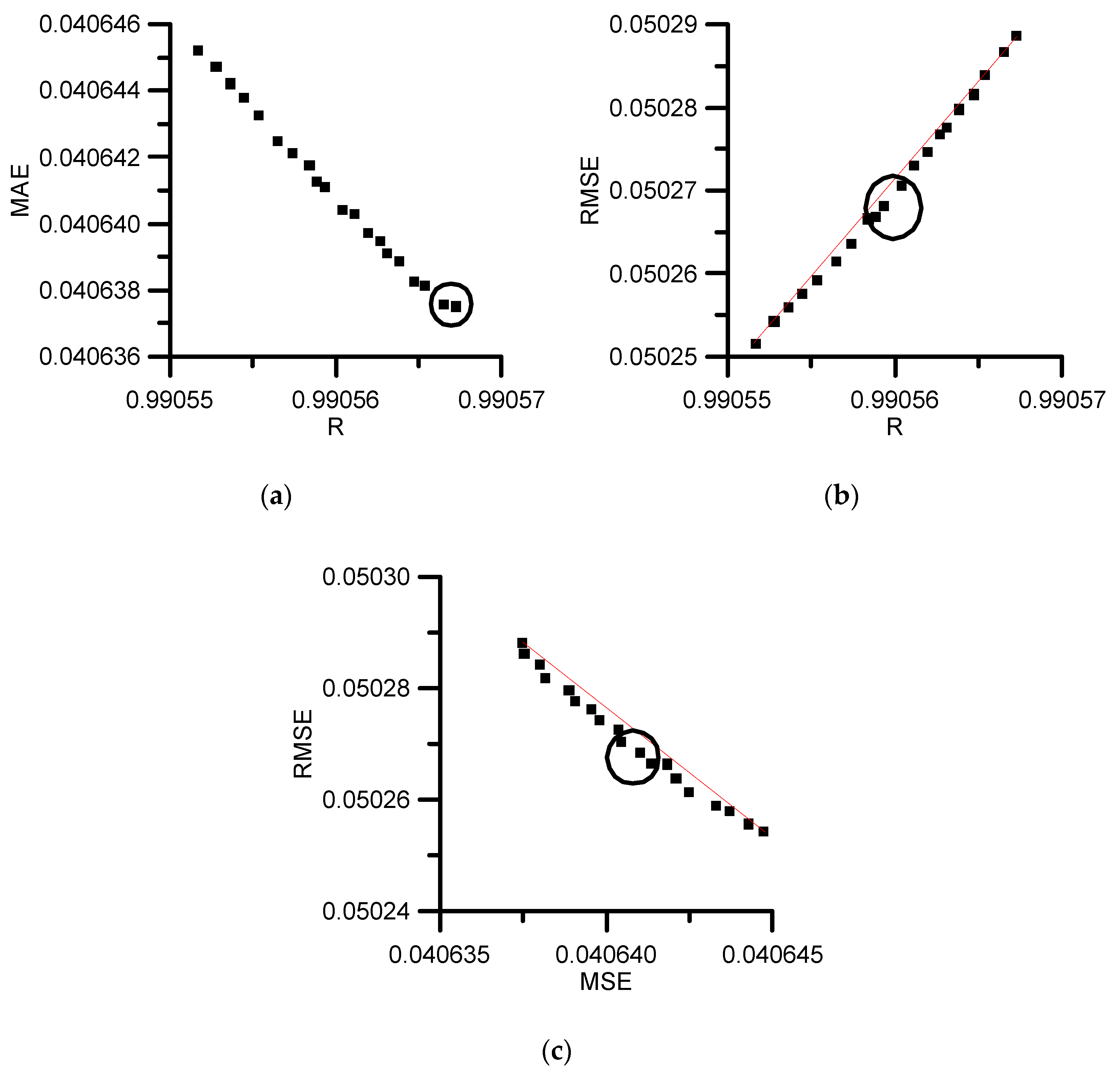
3.2. Optimization of Parameters of the Functions for Determining Bi and D.

The optimization task described by Equation (11) was to search the function constants for evaluation Biot number Bi (aBi, bBi, cBi, dBi, eBi, fBi) and water diffusion coefficient D (aD, bD, cD, dD, eD, fD). The results of the tests are shown in Table 1 and Table 2 and Figure 5.
The best solution for the optimization task is ID S_1 (the greatest R = 0.9905672 and the smallest MAE = 0.0406375). The Biot number for ID S_1 is estimated from the equation:
Bi = 0.7647141 + 10.1689977 s 0.003400086 T + 948.715758 s 2 + 0.000024316 T 2 0.12478256 s T ,
and the water diffusion coefficient:
D = 1.27547936 10 7 2.3808 10 5 s 5.08365633 10 9 T + 0.0030005179 s 2 + 4.266495 10 11 T 2 + 8.33633 10 7 s T
However, the best solution for the smallest RMSE = 0.050252 is ID S_20. The Biot number for ID S_20 is estimated from the equation:
Bi = 0.764714 + 10.1689091 s 0.003400089 T + 948.715738 s 2 + 0.000024316 T 2 0.12478252 s T ,
and the water diffusion coefficient:
D = 1.27547948 10 7 2.3806 10 5 s 5.08365753 10 9 T + 0.0030005175 s 2 + 4.266493 10 11 T 2 + 8.336334 10 7 s T
Considering maximizing R and minimizing both MSE and RMSE, ID S_9 is the best solution (R = 0.9905611; RMSE = 0.050273; MAE = 0.0406403).
The Biot number for ID S_9 is estimated from the equation:
Bi = 0.7647164 + 10.1689997 s 0.003400082 T + 948.715752 s 2 + 0.000024316 T 2 0.12478 s T ,
and the water diffusion coefficient:
D = 1.27547936 10 7 2.3792 10 5 s 5.08365669 10 9 T + 0.0030005201 s 2 + 4.266494 10 11 T 2 + 8.336338 10 7 s T
Model validation was performed. The validation was carried out using new empirical data and it gave good results. These data concerned the drying process of 5 mm thick slices at 45 °C. The R, RMSE and MAE obtained between these data and the model (Equation (4) with Bi and D calculated from (12) and (13), respectively) were 0.9951, 0.0590 and 0.0475, respectively.

4. Conclusions

The paper used a Pareto optimization method for the evaluation of mass diffusion coefficient and mass Biot number, occurring in the equations, describing the drying process. An NSGA algorithm taking into account simultaneous maximization of R and minimization of RMSE and MAE, between the experimental data and model, was satisfactorily used. The optimum Bi, constants of function for Biot number calculation, D and constants of function for mass diffusion coefficient calculation, gained by the NSGA II algorithm, were established. The square type of function f (T,s) can be applied for evaluation of considered Bi and D. The results of statistical analysis for the Bi and D equations were as follows: R = 0.9906, MAE = 0.0406 and RMSE = 0.0503. The conducted model validation gave good results.

Supplementary Materials

The following are available online at https://www.mdpi.com/2073-8994/12/2/260/s1, Table S1: Results of optimization tasks (Pareto optimal set) and considered statistics.

Author Contributions

R.W., formal analysis, optimization, writing of the manuscript; K.G., proposal of the research topic, formal analysis, experiments, modelling, writing of the manuscript; A.K., writing of the manuscript, review and editing. All authors have read and agreed to the published version of the manuscript.

Funding

This research received no external funding.

Conflicts of Interest

The authors declare no conflicts of interest.

Nomenclature

aBi, bBi, cBi, dBi, eBi, fBiconstants in Equation (7) (-)
aD, bD, cD, dD, eD, fDconstants in Equation (8) (-)
Bimass Biot number
Dmass diffusion coefficient (m2 s−1)
kmass transfer coefficient (m s−1)
Lcharacteristic dimension (m)
M, M0, Memoisture content, initial moisture content, equilibrium moisture content (kg H2O kg−1 d.m.)
MR, MRexp, MRpredmoisture ratio, moisture ratio from experiment, predicted moisture ratio (-)
M R ¯ e x p average moisture ratio from experiment
Nnumber of data (-)
shalf of plane (slice) thickness (m)
ttime (s)
Ttemperature (°C)

References

  1. Lewicki, P.P. Water as the determinant of food engineering properties. A review. J. Food Eng. 2004, 61, 483–495. [Google Scholar] [CrossRef]
  2. Doulia, D.; Tzia, K.; Gekas, V. A knowledge base for the apparent mass diffusion coefficient of foods. Int. J. Food Prop. 2000, 3, 1–14. [Google Scholar] [CrossRef]
  3. Gros, J.B.; Ruegg, M. Physical Properties of Foods-2. In COST 90bis Final Seminar Proceedings; Jowitt, R., Escher, F., Kent, M., McKenna, B., Roques, M., Eds.; Elsevier Applied Science: London, UK, 1987; p. 71. [Google Scholar]
  4. Warin, F.; Gekas, V.; Voirin, A.; Dejmek, P. Sugar Diffusivity in Agar Gel/Milk Bilayer Systems. J. Food Sci. 1997, 62, 454–456. [Google Scholar] [CrossRef]
  5. Rattanakijsuntorn, K.; Penkova, A.; Sadha, S.S. Mass diffusion coefficient measurement for vitreous humor using FEM and MRI. IOP Conf. Ser. Mater. Sci. Eng. 2018, 297, 012024. [Google Scholar]
  6. Efremov, G.; Markowski, M.; Białobrzewski, I.; Zielinska, M. Approach to calculation time-dependent moisture diffusivity for thin layered biological materials. Int. Commun. Heat Mass 2008, 35, 1069–1072. [Google Scholar] [CrossRef]
  7. Zamel, N.; Astrath, N.G.C.; Li, X.; Shen, J.; Zhou, J.; Astrath, F.B.G.; Wang, H.; Liu, Z.-S. Experimental measurements of effective diffusion coefficient of oxygen–nitrogen mixture in PEM fuel cell diffusion media. Chem. Eng. Sci. 2010, 65, 931–937. [Google Scholar] [CrossRef]
  8. Chan, C.; Zamel, N.; Li, X.; Shen, J. Experimental measurement of effective diffusion coefficient of gas diffusion layer/microporous layer in PEM fuel cells. Electrochim. Acta 2012, 65, 13–21. [Google Scholar] [CrossRef] [Green Version]
  9. García-Salaberri, P.A.; Hwang, G.; Vera, M.; Weber, A.Z.; Gostick, J.T. Effective diffusivity in partially-saturated carbon-fiber gas diffusion layers: Effect of through-plane saturation distribution. Int. J. Heat Mass Transf. 2015, 86, 319–333. [Google Scholar] [CrossRef] [Green Version]
  10. Wang, Y.; Combe, C.; Clark, M.C. The effects of pH and calcium on the diffusion coefficient of humic acid. J. Membr. Sci. 2001, 183, 49–60. [Google Scholar] [CrossRef]
  11. Stewart, P.S. A Review of Experimental Measurements of Effective Diffusive Permeabilities and Effective Diffusion Coefficients in Biofilms. Biotechnol. Bioeng. 1998, 59, 261–272. [Google Scholar] [CrossRef]
  12. Perré, P.; Pierre, F.; Casalinho, J.; Ayouz, M. Determination of the Mass Diffusion Coefficient Based on the Relative Humidity Measured at the Back Face of the Sample During Unsteady Regimes. Dry Technol. 2015, 33, 1068–1075. [Google Scholar] [CrossRef]
  13. Piot, A.; Woloszyn, M.; Brau, J.; Abele, C. Experimental wooden frame house for the validation of whole building heat and moisture transfer numerical models. Energ. Build. 2011, 43, 1322–1328. [Google Scholar] [CrossRef]
  14. Liu, J.Y.; Simpson, W.T.; Verrill, S.P. An inverse moisture diffusion algorithm for the determination of diffusion coefficient. Dry Technol. 2001, 19, 1555–1568. [Google Scholar] [CrossRef] [Green Version]
  15. Bruin, S.; Luyben, K.C.A.M. Recent developments in dehydration of food materials. In Food Process Engineering; Food processing Systems; Applied Science Publishers: London, UK, 1980; Volume 1. [Google Scholar]
  16. Sitompul, J.P.; Istadi; Widiasa, I.N. Modeling and simulation of deep-bed grain dryers. Dry Technol. 2001, 19, 269–280. [Google Scholar] [CrossRef] [Green Version]
  17. Rovedo, C.O.; Suarez, C.; Viollaz, P. Analysis of moisture profiles, mass Biot number and driving forces during drying of potato slabs. J. Food Eng. 1998, 36, 211–231. [Google Scholar] [CrossRef]
  18. Shi, Q.; Zheng, Y.; Zhao, Y. Mathematical modeling on thin-layer heat pump drying of yacon (Smallanthus sonchifolius) slices. Energy Convers. Manag. 2013, 71, 208–216. [Google Scholar] [CrossRef]
  19. Zielinska, M.; Markowski, M. Drying behavior of carrots dried in a spout–fluidized bed dryer. Dry Technol. 2007, 25, 261–270. [Google Scholar] [CrossRef]
  20. Giner, S.A.; Irigoyen, R.M.T.; Cicuttín, S.; Fiorentini, C. The variable nature of Biot numbers in food drying. J. Food Eng. 2010, 101, 214–222. [Google Scholar] [CrossRef]
  21. Ruiz-López, I.I.; Ruiz-Espinosa, H.; Arellanes-Lozada, P.; Bárcenas-Pozos, M.E.; García-Alvarado, M.A. Analytical model for variable moisture diffusivity estimation and drying simulation of shrinkable food products. J. Food Eng. 2012, 108, 427–435. [Google Scholar] [CrossRef]
  22. Gigler, J.; van Loon, W.K.P.; van der Berg, J.V. Natural wind drying of willow stems. Biomass Bioenerg. 2000, 19, 153–163. [Google Scholar] [CrossRef]
  23. Arévalo-Pinedo, A.; Murr, F.E.X. Kinetics of vacuum drying of pumpkin (Cucurbita maxima): Modeling with shrinkage. J. Food Eng. 2006, 76, 562–567. [Google Scholar] [CrossRef]
  24. Falade, K.O.; Abbo, E.S. Air-drying and rehydration characteristics of date palm (Phoenix dactylifera L.) fruits. J. Food Eng. 2007, 79, 724–730. [Google Scholar] [CrossRef]
  25. Reyes, A.; Mahn, A.; Vásquez, F. Mushrooms dehydration in a hybrid-solar dryer, using a phase change material. Energy Convers. Manag. 2014, 83, 241–248. [Google Scholar] [CrossRef]
  26. Kaleta, A.; Górnicki, K.; Winiczenko, R.; Chojnacka, A. Evaluation of drying models of apple (var. Ligol) dried in a fluidized bed dryer. Energy Convers. Manag. 2013, 67, 179–185. [Google Scholar] [CrossRef]
  27. Saguy, I.S.; Marabi, A.; Wallach, R. New approach to model rehydration of dry food particulates utilizing principles of liquid transport in porous media. Trends Food Sci. Tech. 2005, 16, 495–506. [Google Scholar] [CrossRef]
  28. Sanjuán, N.; Simal, S.; Bon, J.; Mulet, A. Modelling of broccoli stems rehydration process. J. Food Eng. 1999, 42, 27–31. [Google Scholar] [CrossRef]
  29. García-Pascual, P.; Sanjuán, N.; Bon, J.; Carreres, J.E.; Mulet, A. Rehydration process of Boletus edulis mushroom: Characteristics and modelling. J. Sci. Food Agric. 2005, 85, 1397–1404. [Google Scholar] [CrossRef]
  30. García-Pascual, P.; Sanjuán, N.; Melis, R.; Mulet, A. Morchella esculenta (morel) rehydration process modelling. J. Food Eng. 2006, 72, 346–353. [Google Scholar] [CrossRef]
  31. Resio, A.N.C.; Aguerre, R.J.; Suárez, C. Study of some factors affecting water absorption by amaranth grain during soaking. J. Food Eng. 2003, 60, 391–396. [Google Scholar] [CrossRef]
  32. Cunningham, S.E.; Mcminn, W.A.M.; Magee, T.R.A.; Richardson, P.S. Effect of processing conditions on the water absorption and texture kinetics of potato. J. Food Eng. 2008, 84, 214–223. [Google Scholar] [CrossRef]
  33. Maldonado, S.; Arnau, E.; Bertuzzi, M.A. Effect of temperature and pretreatment on water diffusion during rehydration of dehydrated mangoes. J. Food Eng. 2010, 96, 333–341. [Google Scholar] [CrossRef]
  34. Ramallo, L.A.; Albani, O.A. Water diffusion coefficient and modeling of water uptake in packaged yerba mate. J. Food Process. Preserv. 2007, 31, 406–419. [Google Scholar] [CrossRef]
  35. Markowski, M. Air drying of vegetables: Evaluation of mass transfer coefficient. J. Food Eng. 1997, 34, 55–62. [Google Scholar] [CrossRef]
  36. Dincer, I. Moisture transfer analysis during drying of slab woods. Int. J. Heat Mass Transf. 1998, 34, 317–320. [Google Scholar] [CrossRef]
  37. Miketinac, M.J.; Sokhansanj, S.; Tutek, Z. Determination of Heat and Mass Transfer Coefficients in Thin Layer Drying of Grain. Trans. ASAE 1992, 35, 1853–1858. [Google Scholar] [CrossRef]
  38. Wang, N.; Brennan, J.G. A mathematical model of simultaneous heat and moisture transfer during drying of potato. J. Food Eng. 1995, 24, 47–60. [Google Scholar] [CrossRef]
  39. Białobrzewski, I. Determination of the mass transfer coefficient during hot-air-drying of celery root. J. Food Eng. 2007, 78, 1388–1396. [Google Scholar] [CrossRef]
  40. Górnicki, K.; Kaleta, A. Drying curve modelling of blanched carrot cubes under natural convection condition. J. Food Eng. 2007, 82, 160–170. [Google Scholar] [CrossRef]
  41. Huang, C.-H.; Yeh, C.-Y. An inverse problem in simultaneous estimating the Biot numbers of heat and moisture transfer for a porous material. Int. J. Heat Mass Transf. 2002, 45, 4643–4653. [Google Scholar] [CrossRef]
  42. Chen, X.D.; Peng, X. Modified Biot number in the context of air drying of small moist porous objects. Dry Technol. 2005, 23, 83–103. [Google Scholar] [CrossRef]
  43. Li, Z.X.; Renault, F.L.; Gómez, A.O.C.; Sarafraz, M.M.; Khan, H.; Safaei, M.R.; Filho, E.P.B. Nanofluids as secondary fluid in the refrigeration system: Experimental data, regression, ANFIS, and NN modeling. Int. J. Heat Mass Transf. 2019, 144, 118635. [Google Scholar] [CrossRef]
  44. Sarafraz, M.M.; Tlili, I.; Tian, Z.; Bakouri, M.; Safaei, M.R. Smart optimization of a thermosyphon heat pipe for an evacuated tube solar collector using response surface methodology (RSM). Phys. Stat. Mech. Its Appl. 2019, 534, 122146. [Google Scholar] [CrossRef]
  45. Sarafraz, M.M.; Safaei, M.R.; Goodarzi, M.; Arjomandi, M. Experimental investigation and performance optimisation of a catalytic reforming micro-reactor using response surface methodology. Energy Convers. Manag. 2019, 199, 111983. [Google Scholar] [CrossRef]
  46. Benyounis, K.Y.; Olabi, A.G. Optimization of different welding processes using statistical and numerical approaches—A reference guide. Adv. Eng. Softw. 2008, 39, 483–496. [Google Scholar] [CrossRef] [Green Version]
  47. Kopsidas, G. Multiobjective optimization of table olive preparation systems. Eur. J. Oper. Res. 1995, 85, 383. [Google Scholar] [CrossRef]
  48. Kiranoudis, C.; Markatos, N. Pareto design of conveyor-belt dryers. J. Food. Eng. 2000, 46, 145–155. [Google Scholar] [CrossRef]
  49. Therdthai, N.; Zhou, W.; Adamczak, T. Optimization of the temperature profile in bread baking. J. Food. Eng. 2002, 55, 41–48. [Google Scholar] [CrossRef]
  50. Erdogdu, F.; Balaban, M. Complex method for nonlinear constrained optimization of thermal processing multi-criteria. J. Food Process. Eng. 2003, 26, 357–375. [Google Scholar] [CrossRef]
  51. Gergely, S.; Bekassy-Molnar, E.; Vatai, G. The use of multiobjective optimization to improve wine filtration. J. Food Eng. 2003, 58, 311–316. [Google Scholar] [CrossRef]
  52. Hadiyanto, M.; Boom, R.; Straten, G.; Boxtel, A.; Esveld, D. Multi-objective optimization to improve the product range of baking systems. J. Food Process. Eng. 2009, 32, 709–729. [Google Scholar] [CrossRef]
  53. Zhang, Y.; Hidajat, K.; Ray, A.K. Optimal design and operation of SMB bioreactor: Production of high fructose syrup by isomerization of glucose. Biochem. Eng. J. 2004, 21, 111. [Google Scholar] [CrossRef]
  54. Kawajiri, Y.; Biegler, L.T. Nonlinear programming superstructure for optimal dynamic operations of simulated moving bed processes. Ind. Eng. Chem. Res. 2006, 45, 8503. [Google Scholar] [CrossRef]
  55. Hakanen, J.; Kawajiri, Y.; Miettinen, K.; Biegler, L.T. Interactive multi-objective optimization for simulated moving bed processes. Control Cybern. 2007, 36, 50. [Google Scholar]
  56. Abakarov, A.; Sushkov, Y.; Almonacid, S.; Simpson, R. Multiobjective Optimization Approach: Thermal Food Processing. J. Food Sci. 2009, 74, E477–E487. [Google Scholar] [CrossRef] [PubMed]
  57. Winiczenko, R.; Górnicki, K.; Kaleta, A.; Martynenko, A.; Janaszek-Mańkowska, M.; Trajer, J. Multi-objective optimization of convective drying of apple cubes. Comput. Electron. Agric. 2018, 145, 341–348. [Google Scholar] [CrossRef]
  58. Winiczenko, R.; Górnicki, K.; Kaleta, A.; Janaszek-Mankowska, M.; Trajer, J. Multi-objective optimization of the apple drying and rehydration processes parameters. EJFA 2018, 30, 1–9. [Google Scholar]
  59. Seng, C.; Rangaiah, S. Multi-objective optimization in food engineering. In Optimization in Food Engineering; Erdogdu, F., Ed.; Taylor & Francis Book: Abingdon, UK, 2008; Chapter 4; p. 800. [Google Scholar]
  60. Górnicki, K.; Winiczenko, R.; Kaleta, A. Estimation of the Biot Number Using Genetic Algorithms: Application for the Drying Process. Energies 2019, 12, 2822. [Google Scholar] [CrossRef] [Green Version]
  61. Górnicki, K.; Kaleta, A. Modelling convection drying of blanched parsley root slices. Biosyst. Eng. 2007, 97, 51–59. [Google Scholar] [CrossRef]
  62. Luikov, A.V. Analytical Heat Diffusion Theory; Academic Press Inc.: New York, NY, USA, 1970. [Google Scholar]
  63. Crank, J. The Mathematics of Diffusion, 2nd ed.; Clarendon Press: Oxford, UK, 1975; ISBN 978-0-19-853344-3. [Google Scholar]
  64. Pabis, S.; Jayas, D.S.; Cenkowski, S. Grain Drying: Theory and Practice; John Wiley: New York, NY, USA, 1998; ISBN 978-0-471-57387-6. [Google Scholar]
  65. Kaleta, A.; Górnicki, K. Some remarks on evaluation of drying models of red beet particles. Energy Convers. Manag. 2010, 51, 2967–2978. [Google Scholar] [CrossRef]
  66. Kaleta, A.; Górnicki, K. Evaluation of drying models of apple (var. McIntosh) dried in a convective dryer. Int. J. Food Sci. Technol. 2010, 45, 891–898. [Google Scholar] [CrossRef]
  67. Górnicki, K.; Kaleta, A.; Choińska, A. Suitable model for thin-layer drying of root vegetables and onion. Int. Agrophysics 2020, 1, 79–86. [Google Scholar] [CrossRef]
  68. Foneseca, C.M.; Flemming, P. Genetic algorithms for multi-objective optimization: Formulation, discussion, and generalization. In Proceedings of the 5th International Conference on Genetic Algorithms, Urbana-Champaign, July 17–21; Morgan Kaufmann: San Francisco, CA, USA, 1993; pp. 416–423. [Google Scholar]
  69. Deb, K.; Pratap, A.; Agarwal, S.; Meyarivan, T. A fast and elitist multiobjective genetic algorithm: NSGA-II. IEEE Trans. Evol. Comput. 2002, 6, 182–197. [Google Scholar] [CrossRef] [Green Version]
  70. MATLAB 7.6 R2008a, Documentation R; MathWorks, Inc.: Natick, MA, USA, 2008.
Figure 1. Flowchart of the Pareto nondominated sorting genetic algorithm NSGA.
Symmetry 12 00260 g001
Figure 2. Statistics for Pareto optimal sets for Bi, L = 6 mm; thin line—MAE = f (R), dashed line—RMSE = f (R), thick line—RMSE = f (MAE).
Symmetry 12 00260 g002
Figure 3. Statistics for Pareto optimal sets for Bi, T = 70 °C; thin line—MAE = f (R), dashed line—RMSE = f (R), thick line—RMSE = f (MAE).
Symmetry 12 00260 g003
Figure 4. Pareto optimal sets for (a) mass Biot number (Bi) and (b) mass diffusion coefficient (D/s2); L – characteristic dimension, s – half of plane (slice) thickness, T – temperature.
Symmetry 12 00260 g004
Figure 5. Pareto optimal sets for constants in Equations (6) and (7): (a) MAE = f(R), (b) RMSE = f(R), (c) RMSE = f(MSE).
Symmetry 12 00260 g005
Table 1. Pareto optimal set for constants (aBi, bBi, cBi, dBi, eBi, fBi) in Equation (6) and considered statistics; R - coefficient of correlation, MAE - mean absolute error, RMSE - root mean square error.
IDaBibBicBidBieBifBiRRMSEMAE
S_10.764714110.1689977−0.003400086948.7157580.000024316−0.124782560.99056720.0502890.0406375
S_20.764714010.1689891−0.003400089948.7157380.000024316−0.124782520.99056650.0502870.0406376
S_30.764714210.1689057−0.003400089948.7157600.000024319−0.124781290.99056530.0502840.0406381
S_40.764714210.1689752−0.003400082948.7157840.000024316−0.124781960.99056470.0502820.0406383
S_50.764714310.1689954−0.003400083948.7157590.000024317−0.124781020.99056380.0502800.0406389
S_60.764661410.1689890−0.003400072948.7157630.000024330−0.124782770.99056310.0502780.0406391
S_70.764714210.1689346−0.003400066948.7157730.000024316−0.124779510.99056270.0502770.0406395
S_80.764661510.1689980−0.003400071948.7157580.000024330−0.124782140.99056190.0502750.0406397
S_90.764716410.1689977−0.003400082948.7157520.000024316−0.124780000.99056110.0502730.0406403
S_100.764674910.1689859−0.003400075948.7157620.000024323−0.124782590.99056040.0502710.0406404
S_110.764717110.1689683−0.003400077948.7157590.000024316−0.124783680.99055930.0502680.0406411
S_120.764670810.1689920−0.003400071948.7157570.000024324−0.124782740.99055880.0502670.0406412
S_130.764698110.1689694−0.003399883948.7157580.000024320−0.124783350.99055840.0502670.0406418
S_140.764714310.1689797−0.003400077948.7157640.000024316−0.124781100.99055740.0502640.0406421
S_150.764672310.1689885−0.003400092948.7157590.000024324−0.124783620.99055650.0502610.0406425
S_160.764714610.1689610−0.003400070948.7157960.000024316−0.124781250.99055530.0502590.0406432
S_170.764711210.1689946−0.003400011948.7157610.000024316−0.124782720.99055440.0502570.0406438
S_180.764696610.1689920−0.003400075948.7157430.000024323−0.124781890.99055370.0502560.0406442
S_190.764714610.1689886−0.003400073948.7157210.000024317−0.124782610.99055280.0502540.0406447
S_200.764714510.1689228−0.003400067948.7157760.000024316−0.124780940.99055170.0502520.0406452
Table 2. Pareto optimal set for constants (aD, bD, cD, dD, eD, fD) in Equation (7) and considered statistics.
IDaDbDcDdDeDfDRRMSEMAE
S_10.000000127547936−0.000023808−0.000000005083656330.00300051790.000000000042664950.00000083363300.99056720.0502890.0406375
S_20.000000127547948−0.000023806−0.000000005083657530.00300051750.000000000042664930.00000083363340.99056650.0502870.0406376
S_30.000000127547939−0.000023803−0.000000005083656660.00300052160.000000000042664940.00000083363330.99056530.0502840.0406381
S_40.000000127547938−0.000023801−0.000000005083656630.00300048410.000000000042664930.00000083363390.99056470.0502820.0406383
S_50.000000127547934−0.000023799−0.000000005083656800.00300052410.000000000042664930.00000083363340.99056380.0502800.0406389
S_60.000000127547927−0.000023797−0.000000005083657550.00300052750.000000000042664950.00000083363360.99056310.0502780.0406391
S_70.000000127547932−0.000023796−0.000000005083656770.00300052010.000000000042664920.00000083363390.99056270.0502770.0406395
S_80.000000127547934−0.000023794−0.000000005083656710.00300053010.000000000042664940.00000083363370.99056190.0502750.0406397
S_90.000000127547936−0.000023792−0.000000005083656690.00300052010.000000000042664940.00000083363380.99056110.0502730.0406403
S_100.000000127547930−0.000023790−0.000000005083656690.00300051990.000000000042664950.00000083363350.99056040.0502710.0406404
S_110.000000127547935−0.000023787−0.000000005083656340.00300048200.000000000042664930.00000083363320.99055930.0502680.0406411
S_120.000000127547929−0.000023786−0.000000005083656670.00300052670.000000000042664940.00000083363370.99055880.0502670.0406412
S_130.000000127547934−0.000023785−0.000000005083657060.00300052130.000000000042664940.00000083363360.99055840.0502670.0406418
S_140.000000127547935−0.000023782−0.000000005083656940.00300047930.000000000042664930.00000083363370.99055740.0502640.0406421
S_150.000000127547933−0.000023780−0.000000005083657030.00300052650.000000000042664940.00000083363360.99055650.0502610.0406425
S_160.000000127547937−0.000023777−0.000000005083656430.00300049740.000000000042664940.00000083363360.99055530.0502590.0406432
S_170.000000127547934−0.000023775−0.000000005083656670.00300052590.000000000042664940.00000083363370.99055440.0502570.0406438
S_180.000000127547929−0.000023773−0.000000005083656750.00300052270.000000000042664940.00000083363350.99055370.0502560.0406442
S_190.000000127547931−0.000023771−0.000000005083657400.00300053130.000000000042664940.00000083363400.99055280.0502540.0406447
S_200.000000127547938−0.000023768−0.000000005083656540.00300051730.000000000042664930.00000083363330.99055170.0502520.0406452

