A New Flexible Three-Parameter Model: Properties, Clayton Copula, and Modeling Real Data


Abstract
1. Introduction and Motivation
2. Genesis of the New Model
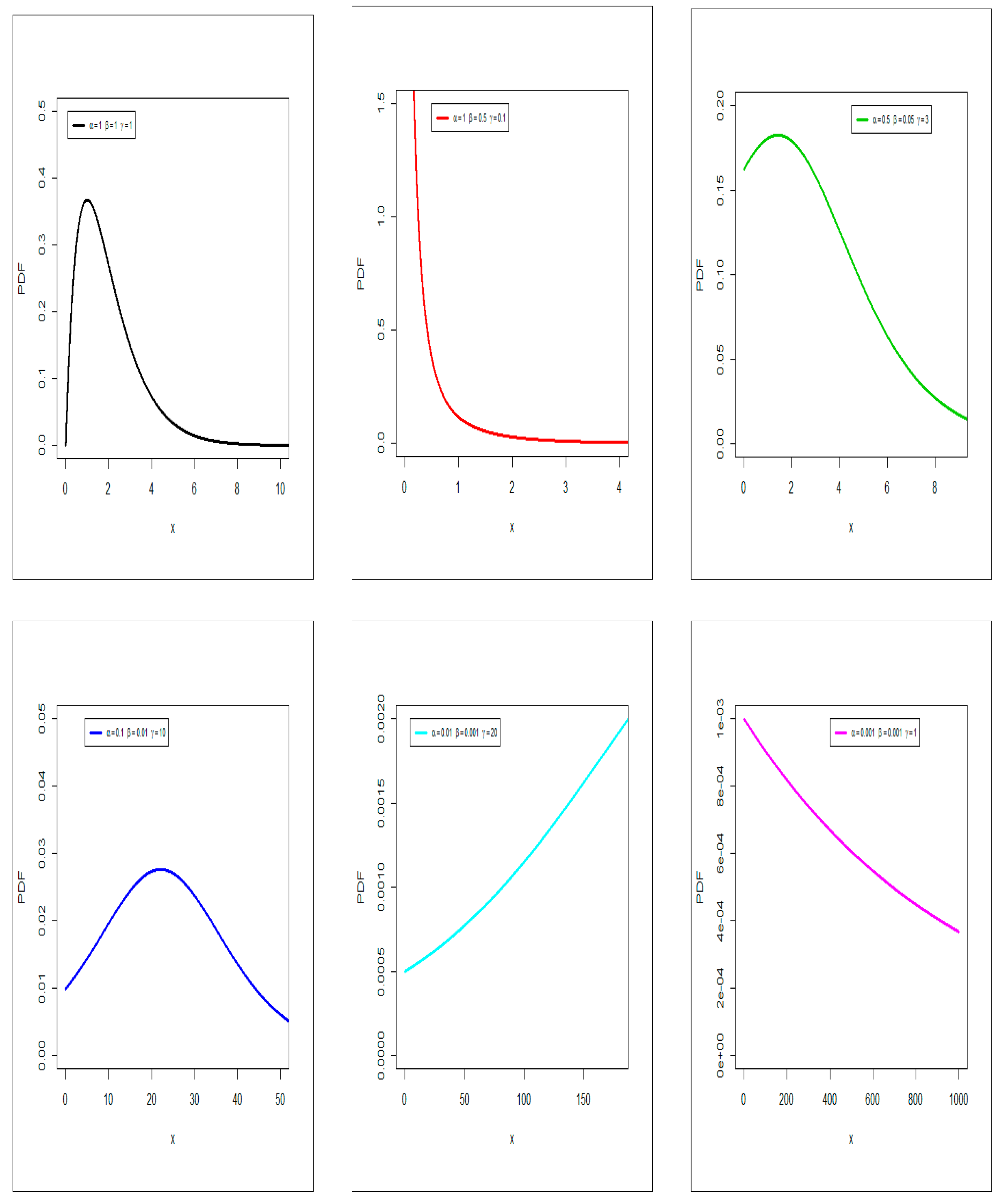
3. Properties
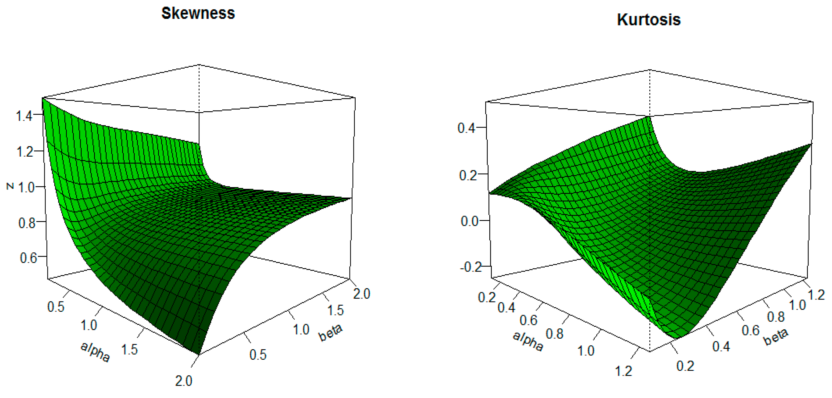
3.1. Moments
3.2. Moment Generating Function (MGF)
3.3. Conditional Moments
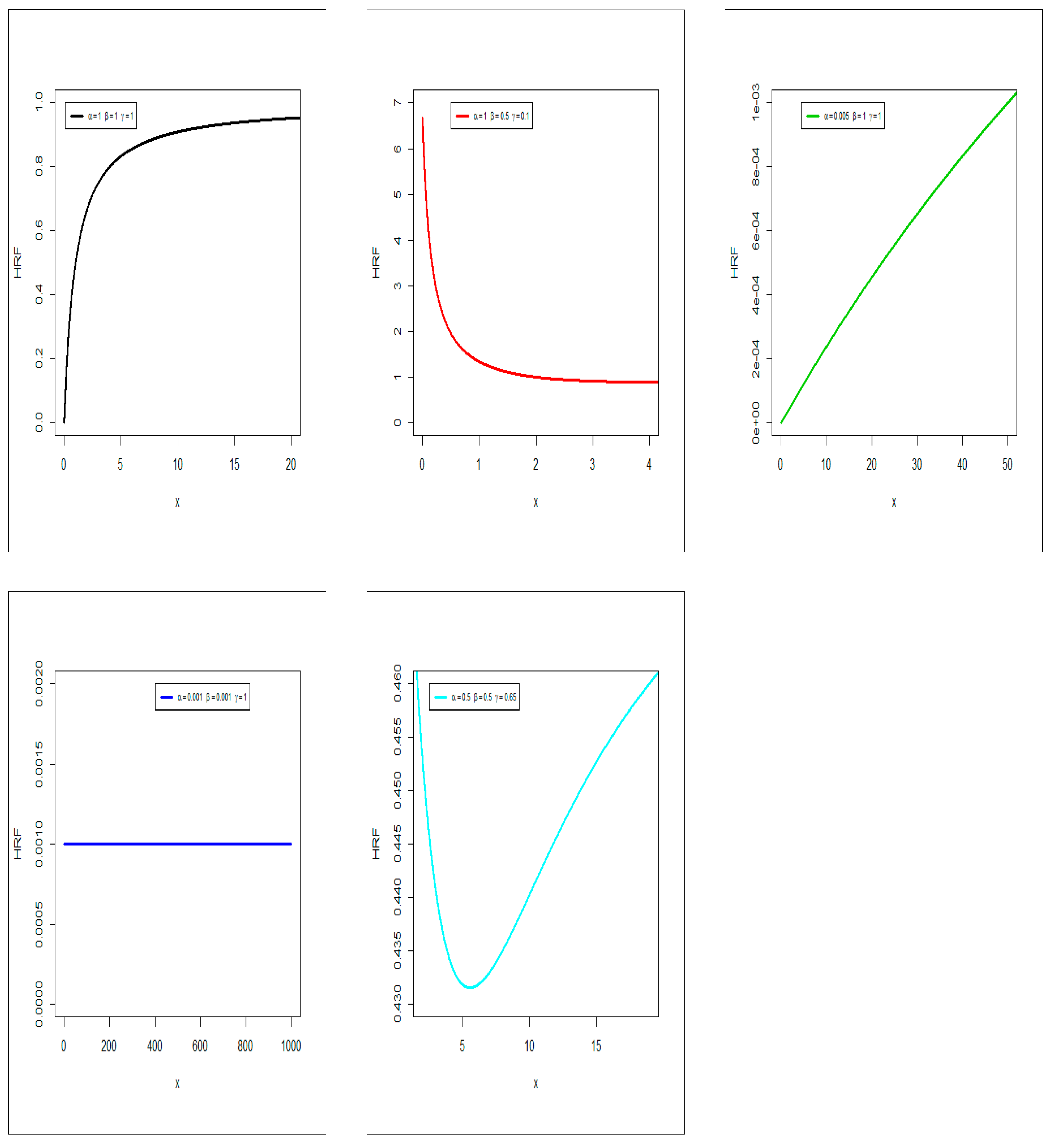
3.4. Residual Life and Reversed Failure Rate Function
4. Simple Type Copula-Based Construction
4.1. The Bivariate MOBE-2 Using the Morgenstern Family
4.2. Via Clayton Copula
4.2.1. The Bivariate MOBE-2 Model
4.2.2. The Multivariate Extension
5. Estimation and Inference
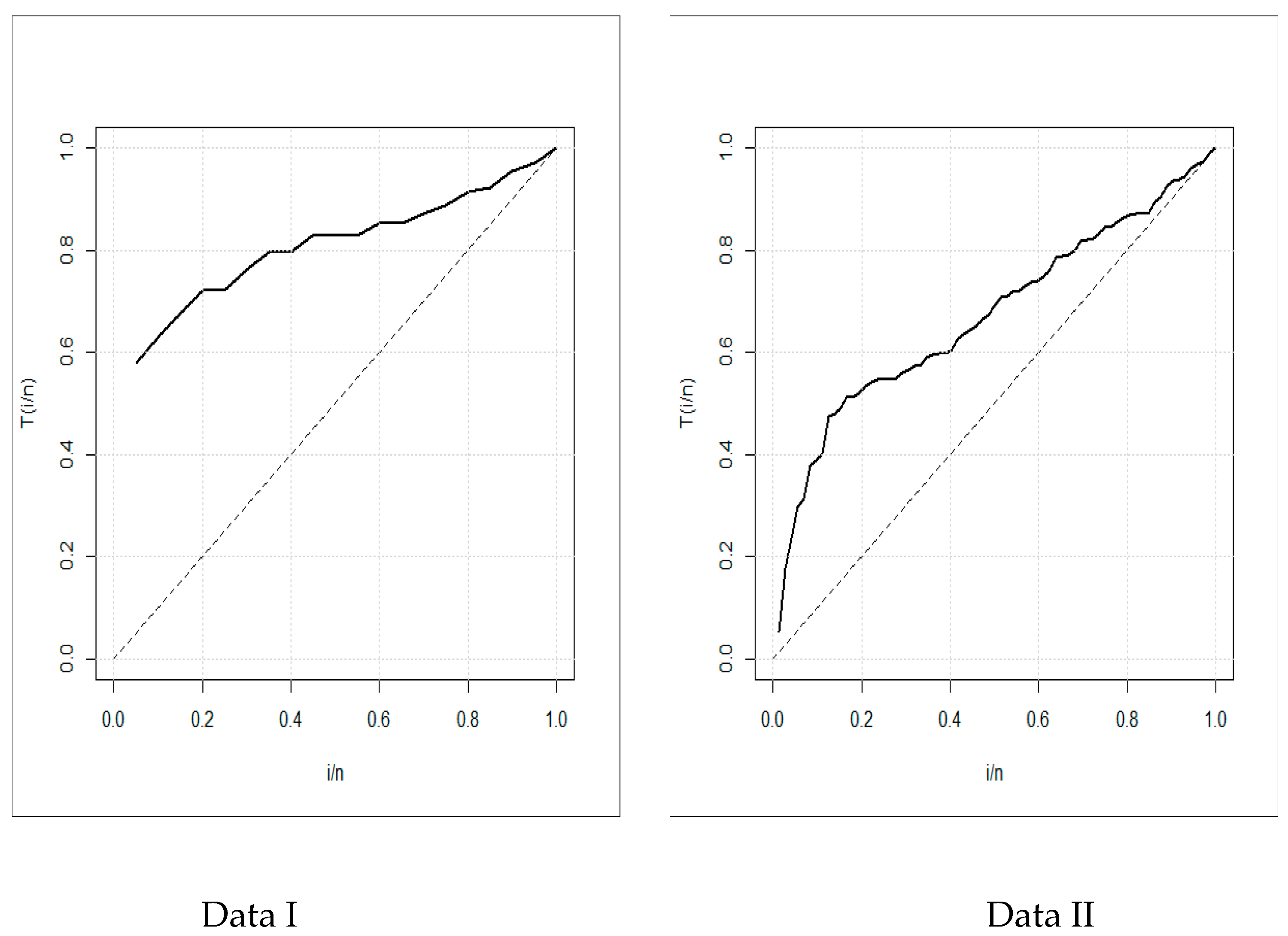
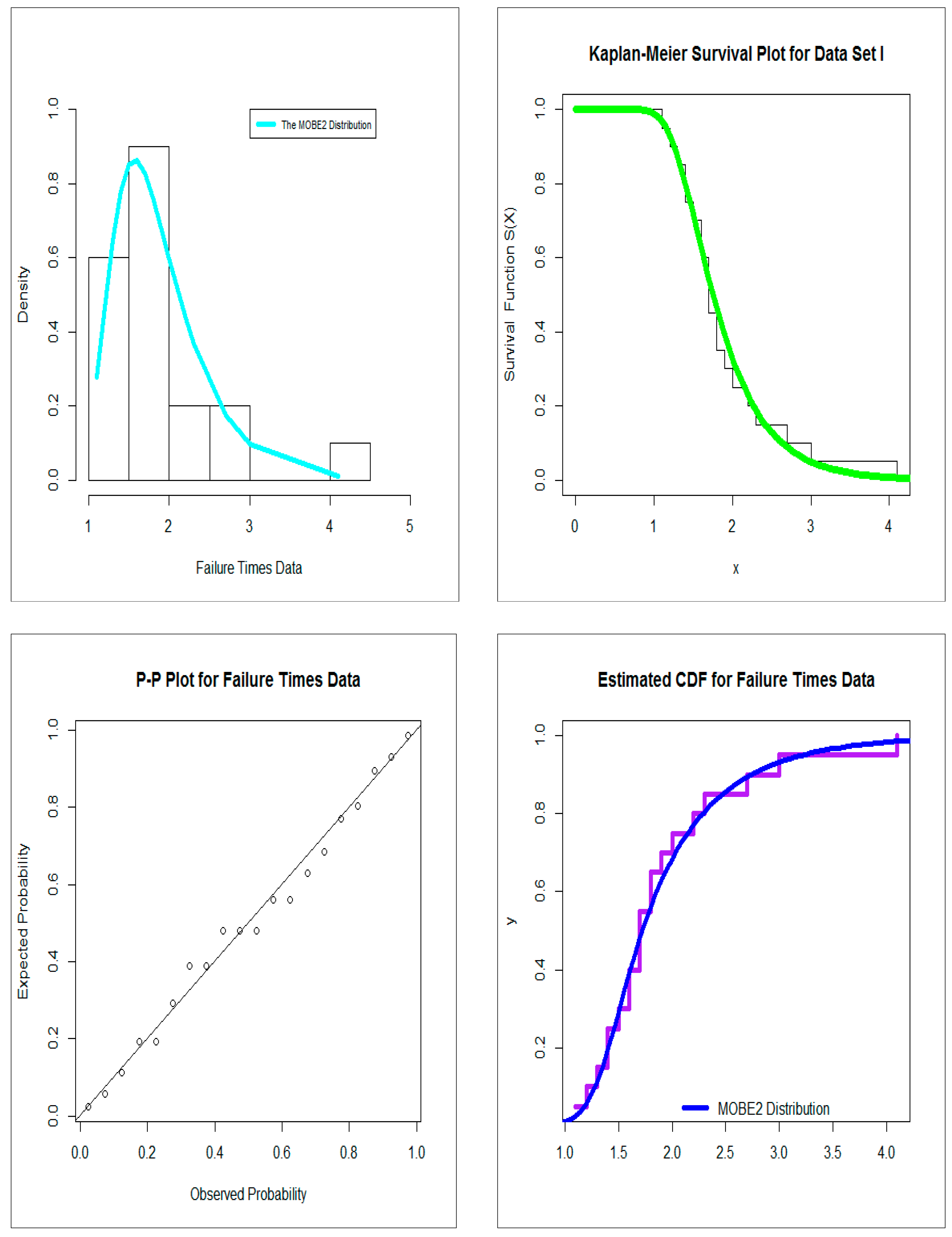
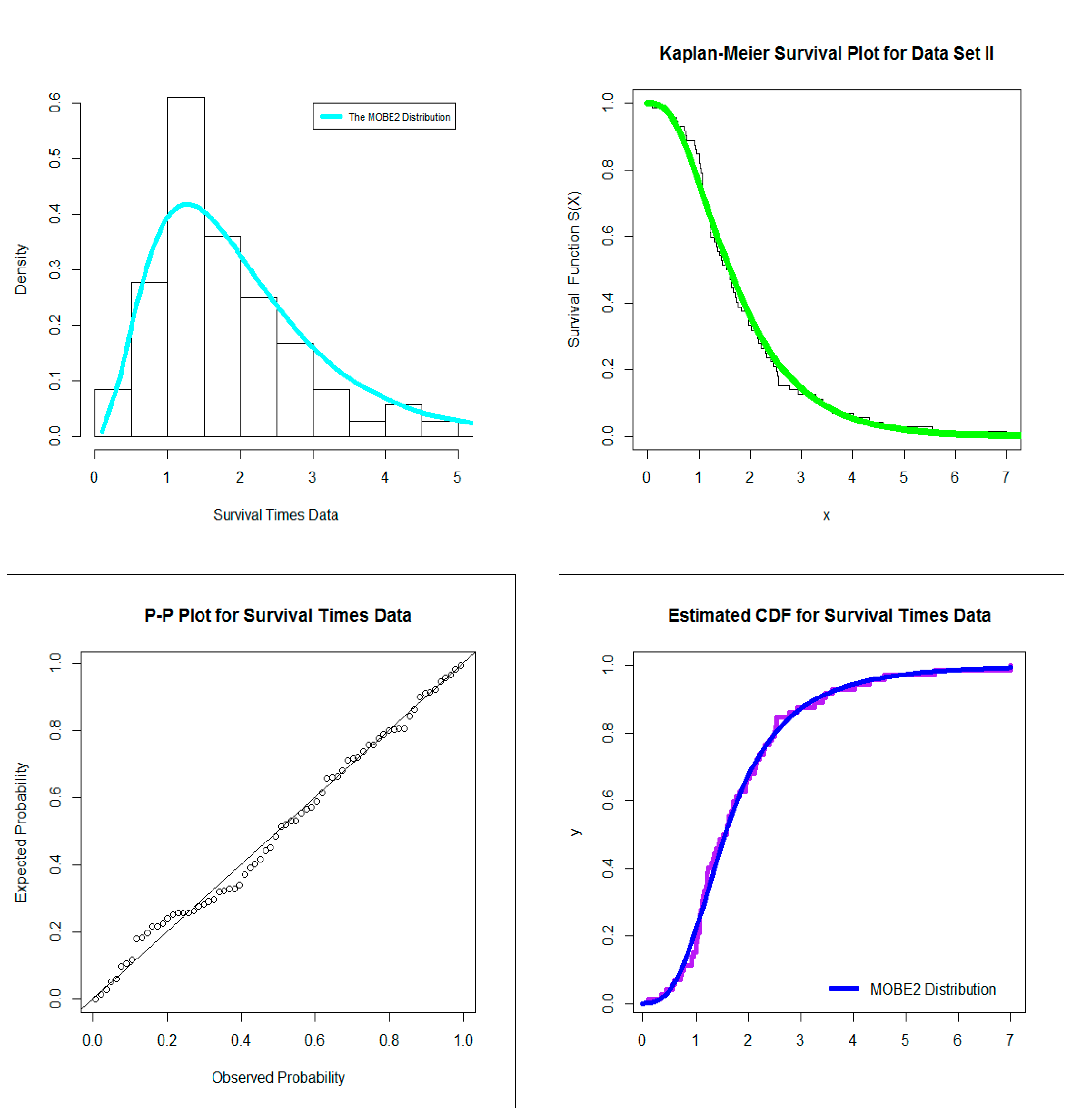
6. Modeling
7. Concluding Remarks
Author Contributions
Funding
Conflicts of Interest
Appendix A
References
- Shaked, M.; Shanthikumar, J. Stochastic Orders; Springer: New York, NY, USA, 2007. [Google Scholar]
- Barlow, R.E.; Proschan, F. Statistical Theory of Reliability and Life Testing; Holt, Rinehart, and Winston: New York, NY, USA, 1975. [Google Scholar]
- Bakouch, S.; Jazi, M.; Nadarajah, S.; Dolati, A.; Roozegar, R. A lifetime model with increasing failure rate. Appl. Math. Model. 2014, 38, 5392–5406. [Google Scholar] [CrossRef]
- Marshall, A.W.; Olkin, I. A new method for adding a parameter to a family of distributions with application to the exponential and Weibull families. Biometrika 1997, 84, 641–652. [Google Scholar] [CrossRef]
- Navarro, J.; Franco, M.; Ruiz, J.M. Characterization through moments of the residual life and conditional spacing. Indian J. Stat. Ser. A 1998, 60, 36–48. [Google Scholar]
- Alizadeh, M.; Ghosh, I.; Yousof, H.M.; Rasekhi, M.; Hamedani, G.G. The generalized odd generalized exponential family of distributions: Properties, characterizations and applications. J. Data Sci. 2017, 15, 443–466. [Google Scholar]
- Yousof, H.M.; Afify, A.Z.; Alizadeh, M.; Nadarajah, S.; Aryal, G.R.; Hamedani, G.G. The Marshall-Olkin generalized-G family of distributions with Applications. Statistica 2018, 78, 273–295. [Google Scholar]
- Yousof, H.M.; Altun, E.; Hamedani, G.G. A new extension of Frechet distribution with regression models, residual analysis and characterizations. J. Data Sci. 2018, 16, 743–770. [Google Scholar]
- Yousof, H.M.; Afify, A.Z.; Alizadeh, M.; Hamedani, G.G.; Jahanshahi, S.M.A.; Ghosh, I. The generalized transmuted Poisson-G family of Distributions. Pak. J. Stat. Oper. Res. 2018, 14, 759–779. [Google Scholar] [CrossRef]
- Yousof, H.M.; Altun, E.; Ramires, T.G.; Alizadeh, M.; Rasekhi, M. A new family of distributions with properties, regression models and applications. J. Stat. Manag. Syst. 2018, 21, 163–188. [Google Scholar] [CrossRef]
- Yousof, H.M.; Butt, N.S.; Alotaibi, R.; Rezk, H.; Alomani, G.A.; Ibrahim, M. A new compound Fréchet distribution for modeling breaking stress and strengths data. Pak. J. Stat. Oper. Res. 2019, 15, 1017–1035. [Google Scholar] [CrossRef]
- Yousof, H.M.; Rasekhi, M.; Altun, E.; Alizadeh, M. The extended odd Frechet family of distributions: properties, applications and regression modeling. Int. J. Appl. Math. Stat. 2018, 30, 1–30. [Google Scholar]
- Nascimento, A.D.C.; Silva, K.F.; Cordeiro, G.M.; Alizadeh, M.; Yousof, H.M. The odd Nadarajah-Haghighi family of distributions: Properties and applications. Stud. Scientiarum Math. Hungarica 2019, 56, 1–26. [Google Scholar] [CrossRef]
- Bantan, R.A.R.; Jamal, F.; Chesneau, C.; Elgarhy, M. Truncated inverted Kumaraswamy generated family of distributions with applications. Entropy 2019, 21, 1089. [Google Scholar] [CrossRef]
- Arshad, R.M.I.; Chesneau, C.; Jamal, F. The odd gamma Weibull-geometric model: Theory and applications. Mathematics 2019, 7, 399. [Google Scholar] [CrossRef]
- Korkmaz, M.C.; Altun, E.; Yousof, H.M.; Hamedani, G.G. The odd power Lindley generator of probability distributions: Properties, characterizations and regression modeling. Int. J. Stat. Probab. 2019, 8, 70–89. [Google Scholar] [CrossRef]
- Korkmaz, M.C.; Yousof, H.M.; Hamedani, G.G. The exponential Lindley odd log-logistic G family: properties, characterizations and applications. J. Stat. Theory Appl. 2018, 17, 554–571. [Google Scholar] [CrossRef]
- Elsayed, H.A.H.; Yousof, H.M. The Burr X Nadarajah Haghighi distribution: Statistical properties and application to the exceedances of flood peaks data. J. Math. Stat. 2019, 15, 146–157. [Google Scholar] [CrossRef]
- Merovci, F.; Alizadeh, M.; Yousof, H.M.; Hamedani, G.G. The exponentiated transmuted-G family of distributions: theory and applications. Commun. Stat.-Theory Methods 2017, 46, 10800–10822. [Google Scholar] [CrossRef]
- Korkmaz, M.C.; Yousof, H.M.; Ali, M.M. Some theoretical and computational aspects of the odd Lindley Fréchet distribution. J. Stat.: Stat. Actuarial Sci. 2017, 2, 129–140. [Google Scholar]
- Ibrahim, M.; Yadav, A.S.; Yousof, H.M.; Goual, H.; Hamedani, G.G. A new extension of Lindley distribution: modified validation test, characterizations and different methods of estimation. Commun. Stat. Appl. Methods 2019, 26, 473–495. [Google Scholar] [CrossRef]
- Idika, E.; Anthony, C.; Johnson, O. Marshall–Olkin generalized Erlange-truncated exponential distribution: Properties and Applications. Cogent Math. 2017, 4, 1–19. [Google Scholar]
- Hamedani, G.G.; Altun, E.; Korkmaz, M.C.; Yousof, H.M.; Butt, N.S. A new extended G family of continuous distributions with mathematical properties, characterizations and regression modeling. Pak. J. Stat. Oper. Res. 2018, 14, 737–758. [Google Scholar] [CrossRef]
- Alizadeh, M.; Rasekhi, M.; Yousof, H.M.; Hamedani, G.G. The transmuted Weibull G family of distributions. Hacet. J. Math. Stat. 2018, 47, 1–20. [Google Scholar] [CrossRef]
- Yadav, A.S.; Goual, H.; Alotaibi, R.M.; Rezk, H.; Ali, M.M.; Yousof, H.M. Validation of the Topp-Leone-Lomax model via a modified Nikulin-Rao-Robson goodness-of-fit test with different methods of estimation. Symmetry 2020, 12, 57. [Google Scholar] [CrossRef]
- Hamedani, G.G.; Rasekhi, M.; Najibi, S.M.; Yousof, H.M.; Alizadeh, M. Type II general exponential class of distributions. Pak. J. Stat. Oper. Res. 2019, 15, 503–523. [Google Scholar] [CrossRef]
- Hamedani, G.G.; Yousof, H.M.; Rasekhi, M.; Alizadeh, M.; Najibi, S.M. Type I general exponential class of distributions. Pak. J. Stat. Oper. Res. 2017, 14, 39–55. [Google Scholar] [CrossRef][Green Version]
- Ibrahim, M. A new extended Fréchet distribution: Properties and estimation. Pak. J. Stat. Oper. Res. 2019, 15, 773–796. [Google Scholar]
- Alizadeh, M.; Yousof, H.M.; Rasekhi, M.; Altun, E. The odd log-logistic Poisson-G Family of distributions. J. Math. Ext. 2019, 12, 81–104. [Google Scholar]
- Ghitany, M.E.; Al-Awadhi, F.A.; Alkhalfan, L.A. Marshall-Olkin extended Lomax distribution and its application to censored data. Commun. Statist. Theor. Meth. 2007, 36, 1855–1866. [Google Scholar] [CrossRef]
- Aryal, G.R.; Yousof, H.M. The exponentiated generalized-G Poisson family of distributions. Econ. Qual. Control 2017, 32, 1–17. [Google Scholar] [CrossRef]


| Models | Estimates |
|---|---|
| E(β) | 0.526 |
| (0.117) | |
| OLiE(β) | 0.6044 |
| (0.0535) | |
| MomE(β) | 0.950 |
| (0.150) | |
| Log BrHE(β) | 0.5263 |
| (0.118) | |
| MOE (α, β) | 54.474, 2.316 |
| (35.582), (0.374) | |
| GMOE (α, α, β) | 0.519, 89.462, 3.169 |
| (0.256), (66.278), (0.772) | |
| KwE(a,b,β) | 83.756, 0.568, 3.330 |
| (42.361), (0.326), (1.188) | |
| BE(a,b,β) | 81.633, 0.542, 3.514 |
| (120.41), (0.327), (1.410) | |
| MOKwE (α, a,b,β) | 0.133, 33.232, 0.571, 1.669 |
| (0.332), (57.837), (0.721), (1.814) | |
| KwMOE (α, a,b,β) | 8.868, 34.826, 0.299, 4.899 |
| (9.146), (22.312), (0.239), (3.176) | |
| BrXE (α, β) | 1.1635, 0.3207 |
| (0.33), (0.03) | |
| MOBE2 (γ, α, β) | 1.83 × 10³, 6.707 × 10⁻², 6.096 × 10⁻³ |
| (2.206 × 10³), (4.991 × 10⁻³), (1.069 × 10⁻³) |
| Models | AIC, BIC, CAIC, HQIC |
|---|---|
| MOBE2 | 40.1, 40.2, 40.3, 39.1 |
| E | 67.67, 68.67, 67.89, 67.87 |
| OLiE | 49.1, 50.1, 49.3, 49.3 |
| MomE | 54.32, 55.31, 54.54, 54.50 |
| Log BrHE | 67.67,68.67,67.89,67.87 |
| MOE | 43.51, 45.51, 44.22, 43.90 |
| GMOE | 42.75, 45.74, 44.25, 43.34 |
| KwE | 41.78, 44.75, 43.28, 42.32 |
| BE | 43.48, 46.45, 44.98, 44.02 |
| MOKwE | 41.58, 45.54, 44.25, 42.30 |
| KwMOExp | 42.8, 46.84, 45.55, 43.60 |
| BrXE | 48.1, 50.1, 8.8, 48.5 |
| Models | , KS and p-Value |
|---|---|
| MOBE2 | 0.33, 0.046, 0.12(0.95) |
| E | 4.60, 0.96, 0.44(0.004) |
| OLiE | 1.3, 0.22, 0.85(6.23 × e−13) |
| MomE | 2.76,0.53, 0.32(0.07) |
| Log BrHE | 0.62, 0.105, 0.44(0.0009) |
| MOE | 0.8, 0.14, 0.1(0.55) |
| GMOE | 0.51, 0.08, 0.15(0.78) |
| KwE | 0.45, 0.07, 0.14(0.86) |
| BE | 0.70, 0.12, 0.16(0.80) |
| MOKwE | 0.60, 0.11, 0.14(0.87) |
| KwMOExp | 1.08, 0.19, 0.15(0.86) |
| BrXE | 1.39, 0.24, 0.248(0.1705) |
| Models | Estimates |
|---|---|
| E(β) | 0.540 |
| (0.063) | |
| OLiE(β) | 0.38145 |
| (0.0209) | |
| MomE(β) | 0.925 |
| (0.077) | |
| Log BrHE(β) | 0.54 |
| (0.064) | |
| MOE (α, β) | 8.778, 1.379 |
| (3.555), (0.193) | |
| GMOE (α, α, β) | 0.179, 47.635, 4.465 |
| (0.070), (44.901), (1.327) | |
| KwE (a, b, β) | 3.304, 1.100, 1.037 |
| (1.106), (0.764), (0.614) | |
| BE (a, b, β) | 0.807, 3.461, 1.331 |
| (0.696), (1.003), (0.855) | |
| MOKwE (α, a, b, β) | 0.008, 2.716, 1.986, 0.099 |
| (0.002), 1.316), (0.784), (0.048) | |
| KwMOE (α, a, b, β) | 0.373, 3.478, 3.306, 0.299 |
| (0.136), (0.861), (0.779), (1.112) | |
| BrXE (α, β) | 0.475, 0.2055 |
| (0.06), (0.012) | |
| MOBE2(γ, α, β) | 11.0365, 0.12054, 0.013601 |
| (4.8066), (0.02246), (0.0077) |
| Models | AIC, BIC, CAIC, HQIC |
|---|---|
| MOBE2 | 207.3, 213.15, 206.6, 209.01 |
| E | 234.63, 236.91, 234.68, 235.54 |
| OLiE | 229.1, 231.4, 229.2, 230 |
| MomE | 210.40, 212.68, 210.45, 211.30 |
| Log BrHE | 234.63, 236.9, 234.7, 235.5 |
| MOE | 210.36, 214.92, 210.53, 212.16 |
| GMOE | 210.54, 217.38, 210.89, 213.24 |
| KwE | 209.42, 216.24, 209.77, 212.12 |
| BE | 207.38, 214.22, 207.73, 210.08 |
| MOKwE | 209.44, 218.56, 210.04, 213.04 |
| KwMOE | 207.82, 216.94, 208.42, 211.42 |
| BrXE | 235.3, 239.9, 235.5, 237.1 |
| Models | , KS, p-Value |
|---|---|
| MOBE2 | 0.68, 0.09, 0.089(0.64) |
| E | 6.53, 1.25, 0.27(0.06) |
| OLiE | 1.94, 0.33, 0.49(9.992 × e−16) |
| MomE | 1.52, 0.25, 0.14(0.13) |
| Log BrHE | 0.71, 0.115, 0.28(2.382 × e−5) |
| MOE | 1.18, 0.17, 0.1(0.43) |
| GMOE | 1.02, 0.16, 0.09(0.51) |
| KwE | 0.74, 0.11, 0.09(0.50) |
| BE | 0.98, 0.15, 0.11(0.34) |
| MOKwE | 0.79, 0.12, 0.10(0.44) |
| KwMOE | 0.61, 0.11, 0.09(0.53) |
| BrXE | 2.9, 0.52, 0.22(0.002) |
© 2020 by the authors. Licensee MDPI, Basel, Switzerland. This article is an open access article distributed under the terms and conditions of the Creative Commons Attribution (CC BY) license (http://creativecommons.org/licenses/by/4.0/).
Share and Cite
A. Al-babtain, A.; Elbatal, I.; M. Yousof, H. A New Flexible Three-Parameter Model: Properties, Clayton Copula, and Modeling Real Data. Symmetry 2020, 12, 440. https://doi.org/10.3390/sym12030440
A. Al-babtain A, Elbatal I, M. Yousof H. A New Flexible Three-Parameter Model: Properties, Clayton Copula, and Modeling Real Data. Symmetry. 2020; 12(3):440. https://doi.org/10.3390/sym12030440
Chicago/Turabian StyleA. Al-babtain, Abdulhakim, I. Elbatal, and Haitham M. Yousof. 2020. "A New Flexible Three-Parameter Model: Properties, Clayton Copula, and Modeling Real Data" Symmetry 12, no. 3: 440. https://doi.org/10.3390/sym12030440
APA StyleA. Al-babtain, A., Elbatal, I., & M. Yousof, H. (2020). A New Flexible Three-Parameter Model: Properties, Clayton Copula, and Modeling Real Data. Symmetry, 12(3), 440. https://doi.org/10.3390/sym12030440