Stability and Convergence Analysis of a Biomagnetic Fluid Flow Over a Stretching Sheet in the Presence of a Magnetic Field

Abstract

This investigated the time-dependent, two-dimensional biomagnetic fluid (blood) flow (BFD) over a stretching sheet under the action of a strong magnetic field. Blood is considered a homogeneous and Newtonian fluid, which behaves as an electrically conducting magnetic fluid that also exhibits magnetization. Thus, a full BFD formulation was considered by combining both the principles of magnetization and the Lorentz force, which arise in magnetohydrodynamics and ferrohydrodynamics. The non-linear governing equations were transformed by using the usual non-dimensional variables. The resulting system of partial differential equations was discretized by applying a basic explicit finite differences scheme. Moreover, the stability and convergence analysis were performed to obtain restrictions that were especially for the magnetic parameters, which are of crucial importance for this problem. The acquired results are shown graphically and were examined for several values of the dimensionless parameters. The flow and temperature distributions were increased as the values of the magnetic parameters were increased. With the progression in time, the flow profile and temperature distribution were also increased. It is hoped that the results of this problem will be used for high targeting efficiency toward determining the maximum values of magnetic field for which accurate flow predictions could be made using a very simple numerical scheme.

1. Introduction

Nowadays, analysis of biomagnetic fluid dynamics (BFD) is more attractive due to the potential biomedical applications. Several applications have been proposed, especially for the medical sciences and bioengineering, including cell separation for magnetic devices, drug delivery using magnetic particles for the treatment of cancer tumors, hyperthermia, and the reduction of bleeding during surgeries [1,2,3,4,5,6,7].

The biofluids, whose flow is influenced by the magnetization and Lorentz force within an external magnetic field, are called biomagnetic fluids. One common biomagnetic fluid is blood, which possesses the properties of a magnetic fluid because of the red blood cells (RBCs). RBCs contain a high concentration of hemoglobin molecules, a form of iron oxide that constitutes a magnetic dipole that is influenced by a magnetic field. Thus, it has been verified [8] that blood could be considered a magnetic fluid. The most important characteristic of a biomagnetic fluid is basically determined by the magnetization force, which also determines how much the magnetic field is affecting the magnetic fluid.

The impact of the magnetization on the flow behavior of blood has been studied by few researchers. The first investigated BFD flows are found in Haik et al. [8]. This BFD model is compatible with the basis of ferrohydrodynamics (FHD) where the induced electric current is considered negligible and the flow is isothermal [9,10]. However, blood is an electrically conducting fluid due to the plasma, which contains ions. Tzirtzilakis [11] proposed an extended BFD model that considers the electrical conductivity of blood. In that study, he adopted both magnetohydrodynamics (MHD) and FHD principles, considering both magnetization and polarization; in addition, he included the energy equation for the investigation of biomedical applications like magnetic hyperthermia.

Crane, in 1970, studied for the first time the classical physical problem of the stretching sheet and presented the solution in an analytical form [12]. Anderson and Valnes [13] demonstrated the impact of a magnetic field that was produced by a magnetic dipole on a ferrofluid passing a stretching sheet. The effect of radiation and magnetization on the ferrofluid passing a stretching sheet was analyzed by Zeeshan et al. [14]. The heat transfer flow of a heated biomagnetic fluid over a nonlinear system was studied by Tzirtzilakis and Kafoussias [15]. Tzirtzilakis and Tanoudis [16] investigated the blood flow through a stretching sheet where they considered blood as a Newtonian fluid. Murtaza et al. [17] studied a steady, incompressible viscous biomagnetic fluid under the effect of an external magnetic field gradient. They considered that the magnetization M is a linear combination of the magnetic field strength H and temperature T. Finally, Ali et al. [18] reported the MHD flow with a stagnation point in the presence of magnetization.

Blood flows in the whole body through capillaries, arteries, and veins. Capillaries carry the blood through the skin and muscles, arteries carry the blood away from the heart, and veins carry the blood toward the heart. Also, we know skins, muscles, arteries, and veins are stretched continuously, and we say that skin and muscles are a stretching surfaces, whereas arteries and veins are a stretching cylinders. Based on the abovementioned analyses, many researchers have conducted their research work evaluting a stretching sheet [15,16,17,18,19].

Albeit a classical physical problem, the analysis of an unsteady stretching sheet is an important topic of ongoing basic research. Das et al. [20] reported the unsteady MHD flow over a stretching sheet and observed that this induced more entropy in the presence of metallic nanoparticles. The unsteady MHD stretching sheet flow was also investigated in three-dimensions by considering velocity and thermal slip boundary conditions [21]. Misra et al. [22] discussed a MHD viscoelastic fluid, which is also electrically conducting, and proposed some applications related to medical sciences, such as hemodynamics.

In the present article, we study unsteady biomagnetic fluid flow over a stretching sheet within the influence of an applied magnetic field generated by a magnetic dipole. Here, we are interested in the flow problem like the one studied before [17] with the consideration of time dependency. Moreover, in the present paper, the mathematical problem is solved using a numerical treatment of the initial set of partial differential equations in conjunction with the previous studies [17], where a similarity problem governed by a system of governing equations with corresponding boundary conditions was solved numerically. For the numerical solution of this problem, we used the finite differences method (FDM) [23]. The stability and convergence analysis were also conducted to determine restrictions for the application of FDM for the values of the magnetic parameters, which are of crucial importance for the flow field. It is hoped that the present study provides some insight of a basic BFD flow configuration for a particularly predicted range of the parameters using a very simple FDM numerical methodology.

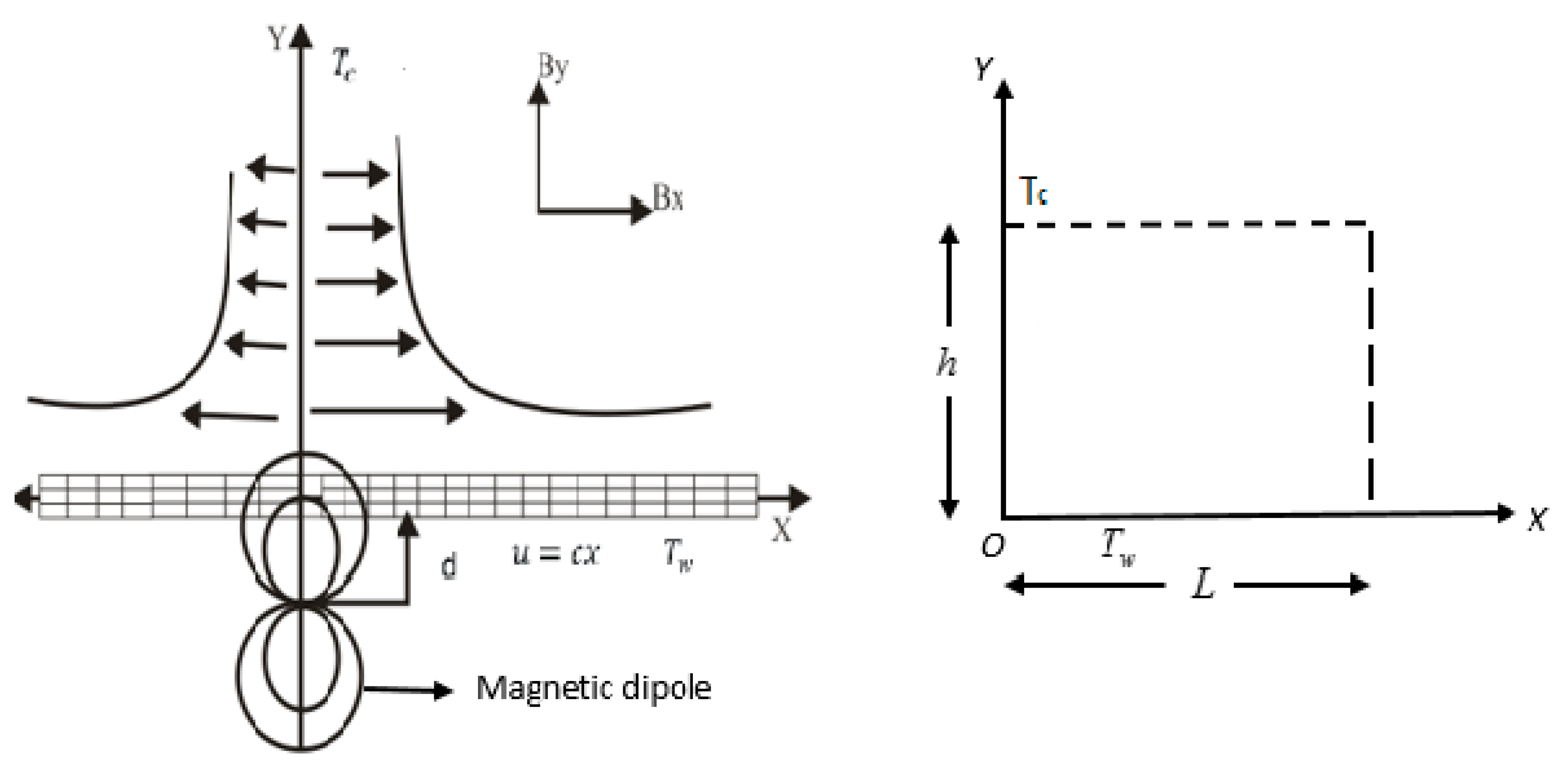
2. Mathematical Model of the Flow

We consider the time-dependent (unsteady), laminar and incompressible viscous fluid (blood) flow past a stretching sheet with velocity $u=cx$, where $c>0$ is a constant. The Cartesian coordinate $x$ is measured along the stretching surface and the coordinate $y$ is normal to the stretching surface. The flow takes place at $y\ge 0$. We also assume that the sheet temperature is $T_w$ and $T_c$ is the ambient temperature, where $T_w<T_c$. A constant pressure gradient $\frac{\partial p}{\partial x}$ and $\frac{\partial p}{\partial y}$ is applied toward the X and Y directions. We also assume that length of the sheet is $l$, and the distance between the ambient temperature and the sheet temperature is $h$. A magnetic dipole that creates a magnetic field is situated below the sheet and the origin of the Cartesian coordinate system (see Figure 1). The magnetic field of the dipole gives rise to a magnetic field of sufficient strength to saturate the biomagnetic fluid. When the biomagnetic fluid enters and leaves the region where the locally applied magnetic field acts and where the gradient of the magnetic field strength is high, the force due to the magnetization, as well as the Lorentz force, arises.

Under the above circumstances, we consider the governing equations, which are valid for the extended BFD model [11,17,24]:

$$\frac{\partial u}{\partial x}+\frac{\partial v}{\partial y}=0$$

(1)

$$\frac{\partial u}{\partial t}+u\frac{\partial u}{\partial x}+v\frac{\partial u}{\partial y}=-\frac{1}{\rho }\frac{\partial p}{\partial x}+\frac{1}{\rho }{\mu }_{0}M\frac{\partial H}{\partial x}-\frac{1}{\rho }\sigma B_y^{2}u+\frac{1}{\rho }\sigma B_x{B}_{y}v+\frac{1}{\rho }\mu \left(\frac{{\partial }^{2}u}{\partial x^2}+\frac{{\partial }^{2}u}{\partial y^2}\right)$$

(2)

$$\frac{\partial v}{\partial t}+u\frac{\partial v}{\partial x}+v\frac{\partial v}{\partial y}=-\frac{1}{\rho }\frac{\partial p}{\partial y}+\frac{1}{\rho }{\mu }_{0}M\frac{\partial H}{\partial y}-\frac{1}{\rho }\sigma B_x^{2}v+\frac{1}{\rho }\sigma B_x{B}_{y}u+\frac{1}{\rho }\mu \left(\frac{{\partial }^{2}v}{\partial x^2}+\frac{{\partial }^{2}v}{\partial y^2}\right)$$

(3)

$$\begin{array}{c}\rho C_p\left(\frac{\partial T}{\partial t}+u\frac{\partial T}{\partial x}+v\frac{\partial T}{\partial y}\right)+{\mu }_{0}T\frac{\partial M}{\partial T}\left(u\frac{\partial H}{\partial x}+v\frac{\partial H}{\partial y}\right)-\sigma B^2{u}^2=k\left(\frac{{\partial }^{2}T}{\partial x^2}+\frac{{\partial }^{2}T}{\partial y^2}\right)\\ +\mu \left[2\left[{\left(\frac{\partial u}{\partial x}\right)}^2+{\left(\frac{\partial v}{\partial y}\right)}^2\right]+{\left(\frac{\partial v}{\partial x}+\frac{\partial u}{\partial y}\right)}^2\right]\end{array}$$

(4)

subject to the following initial and boundary conditions:

$$t\le 0:u=0,v=0,T=T_c\mathrm{everywhere}$$

(5)

$$\begin{array}{c}t>0:u=u(y),v=0,T=T(y)\mathrm{at}x=0\mathrm{and}0\le y\le h\\ u=U_0=cx,v=0,T=T_w\mathrm{at}y=0\mathrm{and}0\le x\le l& u=0,v=0,T=T_c\mathrm{at}y=h(asy\to \infty )\mathrm{or}x=L(\mathrm{as}x\to \infty )y\to \infty \end{array}\}$$

(6)

Here, the velocity components are $q=(u,v)$, $p$ is the pressure, and the other problem parameters, namely $\rho ,\mu ,\sigma ,k,c_p$ are called the biomagnetic fluid density, viscosity, electrical conductivity, thermal conductivity, and specific heat at a constant pressure, respecitvely. Also $B,{\mu }_0,H$ are called the magnetic induction, permeability of the free space, and magnetic field strength intensity, respectively, where $(B={\mu }_{0}H=>\left(B_x,B_y\right)={\mu }_0(H_x,H_y))$.

The additional terms in the Navier–Stokes equations $-\sigma B_y^{2}u+\sigma B_x{B}_{y}v$ and $-\sigma B_x^{2}v+\sigma B_x{B}_{y}u$ represent the Lorentz force per unit volume toward the $x$ and $y$ directions, respectively, and the term represents the Joule heating. For the energy equation, the Joule heating is considered to arise mainly due to the primary velocity u. The abovementioned terms appear due to the electrical conductivity and are well known in MHD [11]. Also, the additional terms of the Naiver–Stokes equations ${\mu }_{0}M\frac{\partial H}{\partial x}$ and ${\mu }_{0}M\frac{\partial H}{\partial y}$ represent the magnetic force due to polarization. The additional term of the energy equation ${\mu }_{0}T\frac{\partial M}{\partial T}\left(u\frac{\partial H}{\partial x}+v\frac{\partial H}{\partial y}\right)$ represents the thermal conductivity per unit volume.

A magnetic dipole produces a magnetic field, whose magnetic scalar is discussed by Andersson and Valnes [13]:

$$V(x,y)=\frac{\alpha }{2\pi }\frac{x}{x^2+{\left(y+d\right)}^2}$$

(7)

The magnitude $\Vert H\Vert =H$ of the magnetic field intensity is that produced by a magnetic dipole [13]

$$H(x,y)={\left(H_x^2+H_y^2\right)}^{\frac{1}{2}}=\frac{\gamma }{2\pi }\frac{1}{x^2+{\left(y+d\right)}^2}$$

(8)

where $\gamma =\alpha$ and $H_x,H_y$ are the components of the magnetic field $\overrightarrow{H}=\left(H_x,H_y\right)$ given by:

$$H_x(x,y)=-\frac{dv}{dx}=\frac{\gamma }{2\pi }\frac{x^2-{\left(y+d\right)}^2}{{\left(x^2+{\left(y+d\right)}^2\right)}^2}$$

(9)

$$H_y(x,y)=-\frac{dv}{dy}=\frac{\gamma }{2\pi }\frac{2x(y+d)}{{\left(x^2+{\left(y+d\right)}^2\right)}^2}$$

(10)

and the gradients are given by:

$$\frac{\partial H}{\partial x}=-\frac{\gamma }{2\pi }\frac{2x}{{\left(y+d\right)}^4}\mathrm{and}\frac{\partial H}{\partial y}=\frac{\gamma }{2\pi }\left(-\frac{2}{{\left(y+d\right)}^3}+\frac{4x^2}{{\left(y+d\right)}^5}\right)$$

(11)

$H$ is the magnetic field strength intensity, which is given by the relation:

$$H(x,y)=\frac{\gamma }{2\pi }\left(\frac{1}{{\left(y+d\right)}^2}-\frac{x^2}{{\left(y+d\right)}^4}\right)$$

(12)

Various relations giving the magnetization M of a biomagnetic fluid are described in Matsuki et al. [25]. Here we use a relation for magnetization involving a combination of $H$ and T:

$$M=KH\left(T_c-T\right)$$

(13)

where K is a constant called the pyromagnetic coefficient.

The magnetic field strength intensity given by Equation (12) can also be achieved by considering the magnetic field generated by a magnetic dipole and taking the expansion of the derivatives close to the origin of the Cartesian system. Clearly, this formulation is valid only very close to the magnetic source and the induced currents are considered negligible to affect the magnetic field itself. These assumptions concerning the mathematical model are described in detail in Tzirtzilakis [11].

3. Mathematical Formulation

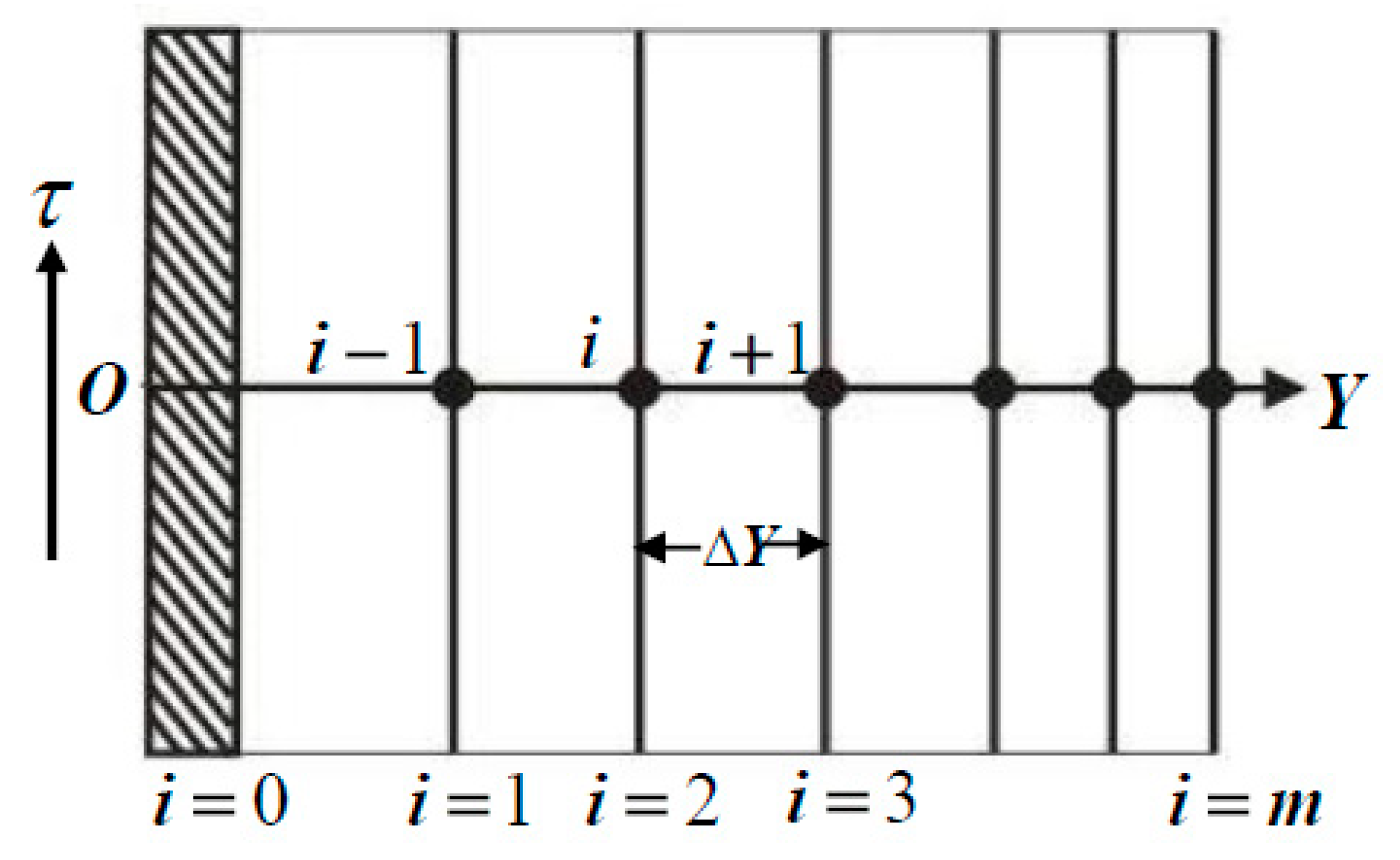
The physical problem described by the governing Equations (1)–(4) subject to the boundary conditions in Equations (5) and (6) were solved using the finite difference method. In order to initiate the solution procedure, we needed to convert the physical problem to the non-dimensional form. Here the following quantities are introduced:

$$X=\frac{x{U}_0}{\nu },Y=\frac{y{U}_0}{\nu },U=\frac{u}{U_0},V=\frac{v}{U_0},P=\frac{p}{\rho U_0^2},\overline{H}=\frac{H}{H_0}$$

$$\overline{H_x}=\frac{H_x}{H_0},\overline{H_y}=\frac{H_y}{H_0},\overline{T}=\frac{T_c-T}{T_c-T_w},\tau =\frac{t{U}_0^2}{\nu }$$

Now after converting to the dimensionless quantities in Equations (1)–(4), the governing equations are transformed to their dimensionless form as follows:

$$\frac{\partial U}{\partial X}+\frac{\partial V}{\partial Y}=0$$

(14)

$$\frac{\partial U}{\partial \tau }+U\frac{\partial U}{\partial X}+V\frac{\partial U}{\partial Y}=-\frac{\partial P}{\partial X}+\left(\frac{{\partial }^{2}U}{\partial X^2}+\frac{{\partial }^{2}U}{\partial Y^2}\right)+M_F\overline{H}\overline{T}\frac{\partial \overline{H}}{\partial X}-M_M{\overline{H}}_y^{2}U+M_M{\overline{H}}_x{\overline{H}}_{y}V$$

(15)

$$\frac{\partial V}{\partial \tau }+U\frac{\partial V}{\partial X}+V\frac{\partial V}{\partial Y}=-\frac{\partial P}{\partial Y}+\left(\frac{{\partial }^{2}V}{\partial X^2}+\frac{{\partial }^{2}V}{\partial Y^2}\right)+M_F\overline{H}\overline{T}\frac{\partial \overline{H}}{\partial Y}-M_M{\overline{H}}_x^{2}V+M_M{\overline{H}}_x{\overline{H}}_{y}U$$

(16)

$$\begin{array}{l}\begin{array}{c}\frac{\partial \overline{T}}{\partial \tau }+U\frac{\partial \overline{T}}{\partial X}+V\frac{\partial \overline{T}}{\partial Y}+M_F{E}_c\overline{H}\left(\epsilon -\overline{T}\right)\left(U\frac{\partial \overline{H}}{\partial X}+V\frac{\partial \overline{H}}{\partial Y}\right)+M_M{E}_c{\overline{H}}^2{U}^2\\ =\left(\frac{1}{P_r}\right)\left(\frac{{\partial }^2\overline{T}}{\partial X^2}+\frac{{\partial }^2\overline{T}}{\partial Y^2}\right)-E_c\left[2\left\{{\left(\frac{\partial U}{\partial X}\right)}^2+{\left(\frac{\partial V}{\partial Y}\right)}^2\right\}+{\left(\frac{\partial V}{\partial X}+\frac{\partial U}{\partial Y}\right)}^2\right]\end{array}\}\end{array}$$

(17)

The corresponding boundary conditions are also transformed to:

$$\tau \le 0:U=0,V=0,\overline{T}=0\mathrm{everywhere}$$

(18)

$$\begin{array}{c}\tau >0:U=0,V=0,\overline{T}=0atX=0\\ U=1,V=0,\overline{T}=1atY=0\\ U=0,V=0,\overline{T}=0asY\to \infty \end{array}\}$$

(19)

where $P_r=\frac{\mu c_p}{k}$ is the Prandtl number, $E_c=\frac{U_0^2}{c_p(T_c-T_w)}$ is the Eckert number, $\epsilon =\frac{T_c}{T_c-T_w}$ is the dimensionless temperature parameter, $M_F=\frac{{\mu }_{0}K{H}_0^2\left(T_c-T_w\right)}{\rho U_0^2}$ is the ferromagnetic (FHD) parameter and $M_M=\frac{\sigma {\mu }_0^2{H}_0^2\nu }{\rho U_0^2}$ is the magnetohydrodynamic (MHD) parameter.

For the MHD parameter we have that $M_M=\frac{\sigma {\mu }_0^2{H}_0^2\nu }{\rho U_0^2}=\frac{\sigma B_0^2{h}^2}{\nu \rho }\frac{{\nu }^2}{h^2{U}_0^2}=\frac{H{a}^2}{{\mathrm{Re}}^2}$, where Ha is the Hartman number known in MHD [26], which express the ratio of the Lorentz forces to the viscous forces. Thus, given that the Re number expresses the ratio of the inertial forces to the viscous forces, the MHD parameter expresses the square of the ratio of the Lorentz forces to the inertial forces. Furthermore, by following analogous considerations in accordance with Davidson [26], we find out that the FHD parameter expresses the ratio of the magnetization forces to the inertial forces. Note that when magnetic parameters $M_F=M_M=0$, then the physical problem is reduced to a simple hydrodynamic fluid problem.

4. Numerical Method

In Section 4, the non-linear partial differential Equations (14)–(17) subject to the boundary conditions in Equations (18) and (19) are treated numerically for the velocity and temperature using the explicit finite differences scheme of Callahan and Marner [27], which is conditionally stable.

In order to solve this problem, we first acquired the difference equation. The boundary layer region was separated into a grid or mesh of lines parallel to the $X$ and $Y$ axes.

We assumed that the maximum length of the plate was $X_{\max }(=100)$ and $Y_{\max }(=10)$ corresponding to $X\to \infty$ and $Y\to \infty$. The grid spacing number was m = 600 and n = 600, as shown in Figure 2. The mesh sizes were considered to be $\Delta X=0.166\left(0<X<100\right)$ and $\Delta Y=0.016\left(0<Y<10\right)$ with a time step $\Delta \tau =0.0001$.

Let $U{}^{\prime },V{}^{\prime }$ and $T{}^{\prime }$ be the new values of $U,V$ and $T$, respectively, at the end of the time step. Applying the explicit finite difference approximation, the following relations are obtained:

$${\left(\frac{\partial U}{\partial \tau }\right)}_{i,j}=\frac{U_{i,j}^{{}^{\prime }}-U_{i,j}}{\Delta \tau },{\left(\frac{\partial U}{\partial X}\right)}_{i,j}=\frac{U_{i,j}-U_{i-1,j}}{\Delta X},{\left(\frac{\partial U}{\partial Y}\right)}_{i,j}=\frac{U_{i,j+1}-U_{i,j}}{\Delta Y}$$

$${\left(\frac{\partial V}{\partial \tau }\right)}_{i,j}=\frac{V_{i,j}^{{}^{\prime }}-V_{i,j}}{\Delta \tau },{\left(\frac{\partial V}{\partial X}\right)}_{i,j}=\frac{V_{i,j}-V_{i-1,j}}{\Delta X},{\left(\frac{\partial V}{\partial Y}\right)}_{i,j}=\frac{V_{i,j+1}-V_{i,j}}{\Delta Y}$$

$${\left(\frac{\partial T}{\partial \tau }\right)}_{i,j}=\frac{{\overline{T}}_{i,j}^{{}^{\prime }}-{\overline{T}}_{i,j}}{\Delta \tau },{\left(\frac{\partial T}{\partial X}\right)}_{i,j}=\frac{{\overline{T}}_{i,j}-{\overline{T}}_{i-1,j}}{\Delta X},{\left(\frac{\partial T}{\partial Y}\right)}_{i,j}=\frac{{\overline{T}}_{i,j+1}-{\overline{T}}_{i,j}}{\Delta Y}$$

$${\left(\frac{{\partial }^{2}T}{\partial X^2}\right)}_{i,j}=\frac{{\overline{T}}_{i+1,j}-2{\overline{T}}_{i,j}+{\overline{T}}_{i-1,j}}{{\left(\Delta X\right)}^2},{\left(\frac{{\partial }^{2}T}{\partial Y^2}\right)}_{i,j}=\frac{{\overline{T}}_{i,j+1}-2{\overline{T}}_{i,j}+{\overline{T}}_{i,j-1}}{{\left(\Delta Y\right)}^2}$$

$${\left(\frac{{\partial }^{2}U}{\partial X^2}\right)}_{i,j}=\frac{U_{i+1,j}-2U_{i,j}+U_{i-1,j}}{{\left(\Delta X\right)}^2},{\left(\frac{{\partial }^{2}U}{\partial Y^2}\right)}_{i,j}=\frac{U_{i,j+1}-2U_{i,j}+U_{i,j-1}}{{\left(\Delta Y\right)}^2},$$

$${\left(\frac{{\partial }^{2}V}{\partial X^2}\right)}_{i,j}=\frac{V_{i+1,j}-2V_{i,j}+V_{i-1,j}}{{\left(\Delta X\right)}^2},{\left(\frac{{\partial }^{2}V}{\partial Y^2}\right)}_{i,j}=\frac{V_{i,j+1}-2V_{i,j}+V_{i,j-1}}{{\left(\Delta Y\right)}^2},$$

By substituting the above relations into Equations (14)–(17), the following Equations are obtained:

$$\frac{U_{i,j}-U_{i-1,j}}{\Delta X}+\frac{V_{i,j+1}-V_{i,j}}{\Delta Y}=0$$

(20)

$$\begin{array}{c}\frac{U_{i,j}^{{}^{\prime }}-U_{i,j}}{\Delta \tau }+U_{i,j}\frac{U_{i,j}-U_{i-1,j}}{\Delta X}+V_{i,j}\frac{U_{i,j+1}-U_{i,j}}{\Delta Y}=-P_1+(\frac{U_{i+1,j}-2U_{i,j}+U_{i-1,j}}{{\left(\Delta X\right)}^2}+\\ \frac{U_{i,j+1}-2U_{i,j}+U_{i,j-1}}{{\left(\Delta Y\right)}^2})+M_F\overline{H}\frac{\partial \overline{H}}{\partial X}{\overline{T}}_{i,j}^{{}^{\prime }}-M_M{\overline{H}}_y^2{U}_{i,j}+M_M{\overline{H}}_x{\overline{H}}_y{V}_{i,j}\end{array}\}$$

(21)

$$\begin{array}{l}\frac{V_{i,j}^{{}^{\prime }}-V_{i,j}}{\Delta \tau }+U_{i,j}\frac{V_{i,j}-V_{i-1,j}}{\Delta X}+V_{i,j}\frac{V_{i,j+1}-V_{i,j}}{\Delta Y}=-P_2+(\frac{V_{i+1,j}-2V_{i,j}+V_{i-1,j}}{{\left(\Delta X\right)}^2}+\\ \frac{V_{i,j+1}-2V_{i,j}+V_{i,j-1}}{{\left(\Delta Y\right)}^2})+M_F\overline{H}\frac{\partial \overline{H}}{\partial Y}{\overline{T}}_{i,j}^{{}^{\prime }}-M_M{\overline{H}}_x^2{V}_{i,j}+M_M{\overline{H}}_x{\overline{H}}_y{U}_{i,j}\end{array}\}$$

(22)

$$\begin{array}{l}\frac{T_{i,j}^{{}^{\prime }}-T_{i,j}}{\Delta \tau }+U_{i,j}\frac{T_{i,j}-T_{i-1,j}}{\Delta X}+V_{i,j}\frac{T_{i,j+1}-T_{i,j}}{\Delta Y}+\epsilon M_F{E}_c\overline{H}\left(U_{i,j}\frac{\partial \overline{H}}{\partial X}+V_{i,j}\frac{\partial \overline{H}}{\partial Y}\right)-M_M{E}_c{\overline{H}}^2{U}_{i,j}^2\\ -M_F{E}_c\overline{H}{\overline{T}}_{i,j}\left(U_{i,j}\frac{\partial \overline{H}}{\partial X}+V_{i,j}\frac{\partial \overline{H}}{\partial Y}\right)=\frac{1}{P_r}\left(\frac{{\overline{T}}_{i+1,j}-2{\overline{T}}_{i,j}+{\overline{T}}_{i-1,j}}{{\left(\Delta X\right)}^2}+\frac{{\overline{T}}_{i,j+1}-2{\overline{T}}_{i,j}+{\overline{T}}_{i,j-1}}{{\left(\Delta Y\right)}^2}\right)-\\ E_c\left[2\left\{{\left(\frac{U_{i,j}-U_{i-1,j}}{\Delta X}\right)}^2+{\left(\frac{V_{i,j+1}-V_{i,j}}{\Delta Y}\right)}^2\right\}+{\left(\frac{V_{i,j}-V_{i-1,j}}{\Delta X}+\frac{U_{i,j+1}-U_{i,j}}{\Delta Y}\right)}^2\right]\end{array}\}$$

(23)

with the corresponding initial and boundary conditions:

$$U_{i,j}^0=V_{i,j}^0={\overline{T}}_{i,j}^0=0$$

(24)

$$\begin{array}{c}{U}_{0,j}^n=V_{0,j}^n={\overline{T}}_{0,j}^n=0\\ U_{i,0}^n=1,V_{i,0}^n=0,{\overline{T}}_{i,0}^n=1\\ U_{i,l}^n=0,V_{i,l}^n=0,{\overline{T}}_{i,l}^n=0wherel\to \infty \end{array}\}$$

(25)

where the subscripts $i$ and $j$ represent the space, and the superscript $n$ represents time. Initially, at $\tau =0$, we considered that the values of $U,V\mathrm{and}\overline{T}$ were known. For any time step, the coefficients $U_{i,j}$ and $V_{i,j}$ appearing in the Equations (20)–(23) behave as constants. For any time step $\Delta \tau$, the new temperature and velocities ${\overline{T}}^{{}^{\prime }}$, $U{}^{\prime }$, and $V{}^{\prime }$ may be obtained by using the continuous process of Equations (20)–(23). This scheme is repeated until the convergence criteria is attained.

5. Stability and Convergence Analysis

The analysis of the convergence and stability provide the necessary basis for the wide range of research on efficient finite difference schemes for problems in mathematical physics. Since the equations are solved using an explicit method, we need to discuss the stability and convergence analysis. The stability and convergence analysis may seem a trivial procedure; however, it is required for every numerical simulation and usually provides restrictions of the values of the physical parameters for which a convergent solution is attained. For this analysis, the stability criteria were established by using fixed mesh sizes as follows.

Equation (20) was ignored since it is not time dependent. For any time $\tau$, we expanded U, V, and T using Fourier series, such that the terms U, V, and T become:

$$\begin{array}{c}U:{\psi }_1(\tau )e^{i\alpha X}{e}^{i\beta Y}\\ V:{\psi }_2(\tau )e^{i\alpha X}{e}^{i\beta Y}\\ \overline{T}:\theta (\tau )e^{i\alpha X}{e}^{i\beta Y}\end{array}\}$$

(26)

Now, Equation (26) can be written after any time step as follows:

$$\begin{array}{c}U:{\psi }_1^{{}^{\prime }}(\tau )e^{i\alpha X}{e}^{i\beta Y}\\ V:{\psi }_2^{{}^{\prime }}(\tau )e^{i\alpha X}{e}^{i\beta Y}\\ \overline{T}:\theta {}^{\prime }(\tau )e^{i\alpha X}{e}^{i\beta Y}\end{array}\}$$

(27)

By substituting Equations (26) and (27) into Equations (21)–(23), and regarding the coefficients U and V as being constant over any time step, after simplification, we can rewrite the Equations as:

$${\psi }_1^{{}^{\prime }}=A_1{\psi }_1+B_1{\psi }_2+C_1\theta {}^{\prime }$$

(28)

$${\psi }_2^{{}^{\prime }}=A_2{\psi }_1+B_2{\psi }_2+C_2\theta {}^{\prime }$$

(29)

$$\theta {}^{\prime }=A_3{\psi }_1+B_3{\psi }_2+C_3\theta$$

(30)

Again, using Equation (30) in Equations (28) and (29), we obtain:

$${\psi }_1^{{}^{\prime }}=A_4{\psi }_1+B_4{\psi }_2+C_4\theta$$

$${\psi }_2^{{}^{\prime }}=A_5{\psi }_1+B_5{\psi }_2+C_5\theta$$

where,

$$A_4=A_1+C_1{A}_3,B_4=B_1+C_1{B}_3,C_4=C_1{C}_3$$

and $A_5=A_2+C_2{A}_3,B_5=B_2+C_2{B}_3,C_5=C_2{C}_3$.

Hence, Equations (28)–(30) can be expressed in matrix notation as follows:

$$\left[\begin{array}{c}{\psi }_1^{{}^{\prime }}\\ {\psi }_2^{{}^{\prime }}\\ {\theta }^{{}^{\prime }}\end{array}\right]=\left[\begin{array}{c}\begin{array}{ccc}{A}_4& B_4& C_4\end{array}\\ \begin{array}{ccc}{A}_5& B_5& C_5\end{array}\\ \begin{array}{ccc}{A}_3& B_3& C_3\end{array}\end{array}\right]\left[\begin{array}{c}{\psi }_1\\ {\psi }_2\\ \theta \end{array}\right]$$

That is ${\eta }^{{}^{\prime }}=T\eta$, where:

$${\eta }^{{}^{\prime }}=\left[\begin{array}{c}{\psi }_1^{{}^{\prime }}\\ {\psi }_2^{{}^{\prime }}\\ {\theta }^{{}^{\prime }}\end{array}\right],T=\left[\begin{array}{c}\begin{array}{ccc}{A}_4& B_4& C_4\end{array}\\ \begin{array}{ccc}{A}_5& B_5& C_5\end{array}\\ \begin{array}{ccc}{A}_3& B_3& C_3\end{array}\end{array}\right]\mathrm{and}\eta =\left[\begin{array}{c}{\psi }_1\\ {\psi }_2\\ \theta \end{array}\right]$$

For the analysis of the stability condition, it is necessary to determine the eigenvalues of the amplification matrix $T$. Since the matrix is third order, it is very difficult to determine the eigenvalues. As an approximation to bypass the above complexity, we considered that the time difference $\Delta \tau$ was very small and tended to zero.

Under this consideration:

$$B_4\to 0,C_4\to 0,A_5\to 0,C_5\to 0,A_3\to 0,B_3\to 0$$

and the amplification matrix becomes:

$$T=\left[\begin{array}{ccc}\begin{array}{c}{A}_4\\ 0\\ 0\end{array}& \begin{array}{c}0\\ B_5\\ 0\end{array}& \begin{array}{c}0\\ 0\\ C_3\end{array}\end{array}\right]$$

After this simplification of the matrix T, we obtain the following eigenvalues:

$${\lambda }_1=A_4,{\lambda }_2=B_5,{\lambda }_3=C_3$$

For the stability analysis, the following conditions for $\left|{\lambda }_n\right|\le 1,n=1,2,3$ must be satisfied:

$$\left|A_4\right|\le 1,\left|B_5\right|\le 1,\left|C_3\right|\le 1\mathrm{for}\mathrm{all}\alpha \mathrm{and}\beta$$

Now we consider:

$$a=U\frac{\Delta \tau }{\Delta X},b=\left|V\right|\frac{\Delta \tau }{\Delta Y},c=2\frac{\Delta \tau }{{\left(\Delta X\right)}^2},d=2\frac{\Delta \tau }{{\left(\Delta Y\right)}^2}$$

where the coefficients a, b, and c are real and non-negative. It has been demonstrated that the maximum modulus of $A_4,B_5\mathrm{and}{C}_3$ occurs when $\alpha \Delta X=m\pi$ and $\beta \Delta Y=n\pi$, where m and n are integers, and hence $A_4,B_5\mathrm{and}{C}_3$ are real. When the values of both m and n are odd integers, then the values of $\left|A_4\right|,\left|B_5\right|\mathrm{and}\left|C_3\right|$ are greater.

To satisfy the condition $\left|C_3\right|\le 1$, the highest negative value is $C_3=-1$, therefore one stability condition is:

$$U\frac{\Delta \tau }{\Delta X}+\left|V\right|\frac{\Delta \tau }{\Delta Y}+\frac{2}{P_r}\left(\frac{\Delta \tau }{{\left(\Delta X\right)}^2}+\frac{\Delta \tau }{{\left(\Delta Y\right)}^2}\right)-\frac{1}{2}{M}_F{E}_c\overline{H}\left(U\frac{\partial \overline{H}}{\partial X}+V\frac{\partial \overline{H}}{\partial Y}\right)\Delta \tau \le 1$$

Therefore, the stability conditions of the method are:

$$U\frac{\Delta \tau }{\Delta X}+\left|V\right|\frac{\Delta \tau }{\Delta Y}+\frac{2}{P_r}\left(\frac{\Delta \tau }{{\left(\Delta X\right)}^2}+\frac{\Delta \tau }{{\left(\Delta Y\right)}^2}\right)-\frac{1}{2}{M}_F{E}_c\overline{H}\left(U\frac{\partial \overline{H}}{\partial X}+V\frac{\partial \overline{H}}{\partial Y}\right)\Delta \tau \le 1$$

(31)

$$\begin{array}{l}U\frac{\Delta \tau }{\Delta X}+\left|V\right|\frac{\Delta \tau }{\Delta Y}+2\left(\frac{\Delta \tau }{{\left(\Delta X\right)}^2}+\frac{\Delta \tau }{{\left(\Delta Y\right)}^2}\right)+\frac{1}{2}{M}_M{\overline{H}}_y^2\Delta \tau +\frac{1}{2}{M}_F\overline{H}\frac{\partial \overline{H}}{\partial X}{[M_M{E}_c\overline{H}}^{2}U+\\ \epsilon M_F{E}_c\overline{H}\frac{\partial \overline{H}}{\partial X}+E_c\left(\frac{8U}{{\left(\Delta X\right)}^2}+\frac{4U}{{\left(\Delta Y\right)}^2}\right)]{\left(\Delta \tau \right)}^2\le 1\end{array}\}$$

(32)

$$\begin{array}{l}U\frac{\Delta \tau }{\Delta X}+\left|V\right|\frac{\Delta \tau }{\Delta Y}+2\left(\frac{\Delta \tau }{{\left(\Delta X\right)}^2}+\frac{\Delta \tau }{{\left(\Delta Y\right)}^2}\right)+\frac{1}{2}{M}_M{\overline{H}}_x^2\Delta \tau +\frac{1}{2}{M}_F\overline{H}\frac{\partial \overline{H}}{\partial Y}[\epsilon M_F{E}_c\overline{H}\frac{\partial \overline{H}}{\partial Y}\\ +E_c\left(\frac{8V}{{\left(\Delta Y\right)}^2}+\frac{4V}{{\left(\Delta X\right)}^2}-\frac{8U}{\Delta X.\Delta Y}\right)]{\left(\Delta \tau \right)}^2\le 1\end{array}\}$$

(33)

Using the initial condition, $U=V=\overline{T}=0$ at $\tau =0,$ we determined the stability and convergence criteria of the method to be $P_r\ge 0.733,M_F\le 1.73\times {10}^8$, and $M_M\le 2.1\times {10}^4.$ (Appendix A).

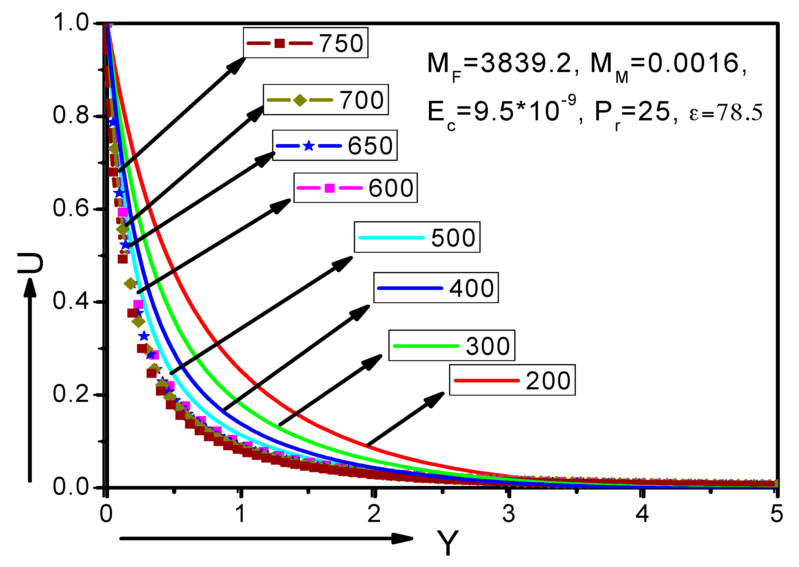
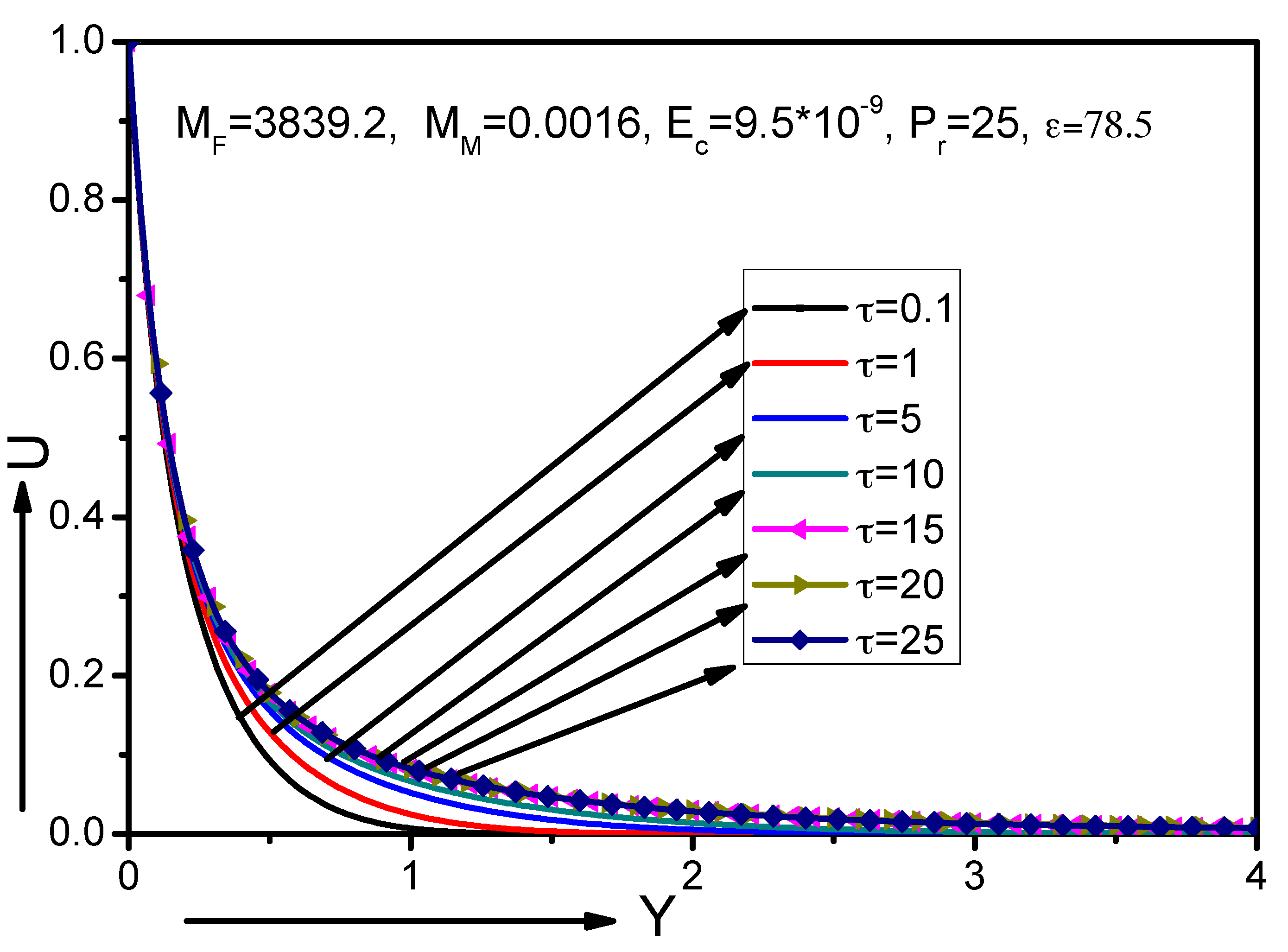
6. Results and Discussion

6.1. Justification of the Grid Space

To verify the independence of the obtained results on the grid used, i.e., from the grid $m\times n$ toward the X and Y directions, respectively, the code was run with a different space grids, namely $m=n=200,m=n=300,m=n=400,m=n=500,m=n=600,$ $m=n=700$, and $m=n=750$. It was found that the grid independency was achieved at about $m=n=600$ where minor changes were observed in comparison with the solution attained for $m=n=750$. A characteristic grid independency check is pictured in Figure 3 where the velocity no longer changed for $m=n=600$ and denser grids.

6.2. Steady-State Solution

For the steady-state solution, calculations were repeated up to non-dimensional time $\tau =25$. The major changes in the prime variables occurred up to the dimensionless time $\tau =10$, and minor changes occurred for $\tau =10\mathrm{to}25$. Thus, the solution for dimensionless time $\tau =25$ was considered the steady-state solution for this problem. Figure 4 shows a representative solution of the U velocity profile for different time steps and for grid points $m=600,n=600$. It was found that the velocity increased gradually as the time increased, until the steady-state $\left(\tau =25\right)$ condition was attained. For the steady-state solutions of all quantities presented, a check similar to the one mentioned above was performed to ensure that the solution depicted was indeed a steady-state solution.

6.3. Estimation of Parameters

For the solution procedure, we needed to assign some numerical values to the problem parameters. Since we adopted blood as the fluid in question, we considered the fluid to hold the properties of blood with a density $\rho =1050\mathrm{kg}{\mathrm{m}}^{-3}$ and viscosity $\mu =3.2\times {10}^{-3}\mathrm{kg}{\mathrm{m}}^{-1}{\mathrm{s}}^{-1}$, flowing with a maximum velocity $U_0=1.22\times {10}^{-2}\mathrm{m}{\mathrm{s}}^{-1}$ [16]. Also, we took $\sigma =0.8{\mathrm{s}\mathrm{m}}^{-1}$ [28], $c_p=3.9\times {10}^3{\mathrm{J}\mathrm{kg}}^{-1}{\mathrm{K}}^{-1}$, and $k=0.5{\mathrm{J}\mathrm{m}}^{-1}{\mathrm{s}}^{-1}{\mathrm{K}}^{-1}$ [17]. The sheet temperature was considered to be $T_w=37°\mathrm{C}$, while the ambient temperature was $T_c=41°\mathrm{C}$. Using these values, we calculated the dimensionless temperature number to be $\epsilon =78.5$ and the Prandtl number to be $P_r=25$.

Now, we rewrite the ferromagnetic $\left(M_F\right)$ and magnetohydrodynamic numbers $\left(M_M\right)$ as

$$M_F=\frac{{\mu }_{0}K{H}_0^2\left(T_c-T_w\right)}{\rho U_0^2}=\frac{{\mu }_0{H}_{0}K{H}_0\left(T_c-T_w\right)}{\rho U_0^2}=\frac{B_0{M}_0}{\rho U_0^2}$$

and

$$M_M=\frac{\sigma {\mu }_0^2{H}_0^2\nu }{\rho U_0^2}=\frac{\sigma B_0^2\nu }{\rho U_0^2}$$

(34)

where B₀ and M₀ are the magnetic induction number and magnetization number, respectively. For pure blood, it has been found that the saturation magnetization of $60{\mathrm{Am}}^{-1}$ is attained for a magnetic field strength above 6 T [8,11]. It is possible to attain order of magnitudes greater magnetization artificially, i.e., via the addition of magnetic nanoparticles, using much lower magnetic field strengths, such as 1 T or even less. The electrical conductivity of blood could also be artificially increased, and thus, the range of values of $M_F$ and $M_M$ could vary significantly depending on the specific application. For the present case, we considered some reference values of the magnetic field induction B₀, and we considered $M_F$ and $M_M$ as determined by Equation (34). It is apparent that someone could arrive at totally different values depending on a specialized application, such as reinforcing polarization or electrical conductivity, by adding magnetic nanoparticles or electrolytes, respectively. Some corresponding values of ferromagnetic $\left(M_F\right)$ and magnetohydrodynamic $\left(M_M\right)$ numbers with a reference magnetic induction are given in

Table 1. Reference magnetic field induction and corresponding values of $M_F$ and $M_M$.

$\mathbf{Reference}\mathbf{Magnetic}\mathbf{Field}\mathbf{Flux}(\overrightarrow{\mathit{B}})$	Magnetohydrodynamic Number (MM)	Ferromagnetic Number (MF)
2 T	0.000062	767.8
4 T	0.00025	1535.5
6 T	0.00056	2303.5
8 T	0.001	3071.2
9 T	0.0013	3455.1
10 T	0.0016	3839.2

.

Considering the above case scenario of the physical problem, as well as the above analysis of the magnetic numbers, we derived representative values for the Eckert number $E_c=9.5\times {10}^{-9}$; Prandtl number $P_r=25$; magnetohydrodynamic (MHD) number $M_M=$ $0,0.0016,0.001,0.00056,0.00025,0.000062$; and ferromagnetic (FHD) number $M_F=0,3839.2,3071.2,2303.5,1535.5,767.8$. We found that the abovementioned stability analysis gave the restrictions for the parameters, which were ${\mathrm{P}}_r\ge 0.733,M_F\le 1.73\times {10}^8$, and $M_M\le 2.1\times {10}^4.$ Thus, the values adopted for the above case scenario of the physical problem were well below the values of the ferromagnetic $\left(M_F\right)$ and magnetohydrodynamic $\left(M_M\right)$ numbers required for the validity of the numerical method stability. However, as it has already been noted, these limiting values of the ferromagnetic $\left(M_F\right)$ and magnetohydrodynamic $\left(M_M\right)$ numbers should kept in mind for the investigation of BFD flow problems where the polarization is controlled by the addition of magnetic nanoparticles.

In order to assess the validity and accuracy of the numerical results, we computed the Nusselt number for the steady-state condition with $M_F=0,M_M=0,H=H_x=H_y=P=E_c=0$, and compared them with Khan et al. [29] in

Table 2. Comparison of the Nusselt number for different values of $P_r$ with $M_F=0,M_M=0,H=H_x=H_y=P=E_c=0$.

${\mathit{P}}_{\mathit{r}}$	Present Result	Khan et al. [29]
0.2	0.1689	0.1694
0.7	0.4524	0.4544
2	0.909	0.9109
7	1.8930	1.8960
20	3.3532	3.3541

and observed that our results were in excellent agreement with those of Khan et al. [29]. Therefore, we conclude that our observation method was accurate in light of this comparison.

The effect of the magnetohydrodynamic and ferromagnetic parameters on the velocities U and V, and the temperature distribution T are shown in Figure 5, Figure 6 and Figure 7. It is observed from Figure 5, Figure 6 and Figure 7 that the fluid primary velocity and temperature distribution decreased with the increase of the MHD and FHD parameter, whereas the corresponding secondary velocities increased. This fact was due to the presence of a magnetic field, which is also called the Kelvin force, which acts against the flow. This resistive force slows down the fluid velocity component.

This abovementioned phenomenon pictured in Figure 5 and Figure 6, i.e., the decrease of the primary velocity with the simultaneous increase of the corresponding secondary ones as the magnetic field strength intensity increased, has also been observed in numerous BFD studies [11,13,15,17]. The increase in the secondary velocity was maximized at about Y = 1, and after that point, begins to decay, forming a bell-shaped distribution. For BFD problems of internal flows, it is a generally found that the formation of a vortex close to the area of the application of the magnetic field depends on the geometry of the physical plane and the magnetic field strength and gradient [11]. It seems that this vortex-like phenomenon tends to appear in the analogous stretching sheet boundary layer problems, emerging with an increase of the secondary velocity close to the magnetic source. This increase is always local, and finally, the secondary velocity distribution decays, forming a characteristic bell-shaped distribution through the boundary layer [13,15,17]. Moreover, Figure 5 and Figure 6 depict the distributions of the primary and secondary velocities for various magnetic field strengths for τ = 0.1, apart from that of τ = 15, which corresponds to the steady state. It was found that, as the time elapsed, the effect of the magnetic field on the flow was analogous to that observed on the final, steady state. Clearly, for a specific τ, the primary velocity u was reduced with the induction of the magnetic field intensity, whereas the secondary velocity v rose and was increased as the magnetic field strength also increased.

The variation of the dimensionless temperature T with Y is pictured in Figure 7. The dimensionless temperature was generally reduced at the area of the boundary layer as the magnetic field strength increased. It was apparent that the decrease of the dimensionless temperature meant an increase of the corresponding dimensional one. For greater values of the magnetic field in the steady state and for 1 < Y < 3, the dimensionless temperature had small negative values, which meant that the dimensional temperature was greater than that of the corresponding hydrodynamic case. This phenomenon was enhanced as the time passed toward the steady state. For smaller times, as for τ = 0.1, the temperature variation was confined in a smaller region in the boundary layer. Specifically, for τ = 0.1, the region of variation of the dimensionless temperature was Y < 1. Generally, the application of the magnetic field, at any time, had the influence of dropping the dimensionless temperature more rapidly than in the corresponding hydrodynamic case.

Another important flow characteristic concerning stretching sheet flow problems are the missing slope, which is also known as a skin friction and the rate of heat transfer coefficient as defined by the following relations [12,13,15,17]:

$C_{f_x}=-\frac{2{\tau }_w}{\rho {\left(cx\right)}^2}$, where ${\tau }_w=\mu {\frac{\partial u}{\partial y}|}_{y=0}$ is the wall shear stress, and $N{u}_x=\frac{x}{T_c-T_w}{\frac{\partial T}{\partial y}|}_{y=0}$, where $N{u}_x$ is the local Nusselt number.

Using the non-dimensional variables from Section 2, we concluded that the above quantities can be written as:

$C_{f_x}=-2c{\frac{\partial U}{\partial Y}|}_{Y=0}$ and $N{u}_x=X{\frac{\partial \overline{T}}{\partial Y}|}_{Y=0}$, where we can define ${\frac{\partial U}{\partial Y}|}_{Y=0}$ as the dimensionless wall shear parameter and ${\frac{\partial \overline{T}}{\partial Y}|}_{Y=0}$ as the dimensionless wall heat transfer parameter.

The change of the dimensionless wall shear parameter $-{\frac{\partial U}{\partial Y}|}_{Y=0}$, for the steady state, is shown in Figure 8. Here, we observed that the wall shear parameter varied nonlinearly with the distance X, regardless of the application of the magnetic field. We also observed that the values of the wall shear parameter increased as the strength of magnetic field increased. For grater values of the magnetic field strength, the values of this coefficient for X > 2 increased by more than 100% compared to the hydrodynamic case. This was justified because the application of the magnetic field for this kind of problems generally involves rising forces opposing the main flow direction; this also coincides with previously published results [13,15,16,17].

The variation of the wall heat transfer parameter for various values of magnetic field strength for the steady state is pictured in Figure 9. Generally, the variation of the wall heat transfer parameter with X was a nonlinear reduction. The increase of the magnetic field resulted in an increase of the wall heat transfer parameter. It seems that the increase of the dimensionless wall shear parameter observed in Figure 8 was related to an analogous increase of the dimensionless wall heat transfer parameter. For the steady state and for approximately X > 2, the increase of this coefficient was also beyond 150% for greater values of the magnetic field strength.

These results were extensive enough and the addition of two-dimensional results had nothing to add as far as the solution of the physical problem itself was concerned. If one observes the solution with respect the second direction, for these values of the parameters, it was shown that the solution actually follows a similar pattern. Therefore, it is concluded that adding the solution toward the second dimension had nothing to add other than complexity. On the other hand, the results were presented as one dimensional because for this type of problem, the majority of the derived results are one dimensional. Therefore, if the reader wants, they could perform calculations comparing the present results with results obtained from a reduced problem as described by a system of ordinary differential equations along with the corresponding boundary conditions as was used when the one-dimensional reduction was applied.

7. Conclusions

The BFD unsteady stretching sheet flow was studied. The numerical treatment was made using an explicit finite difference method (EFDM) with an elaborated stability and convergence analysis. The values of the key parameters corresponding to a physical case scenario were well in the range required for the stability and convergence of the numerical scheme. The computations for the steady state have shown the following:

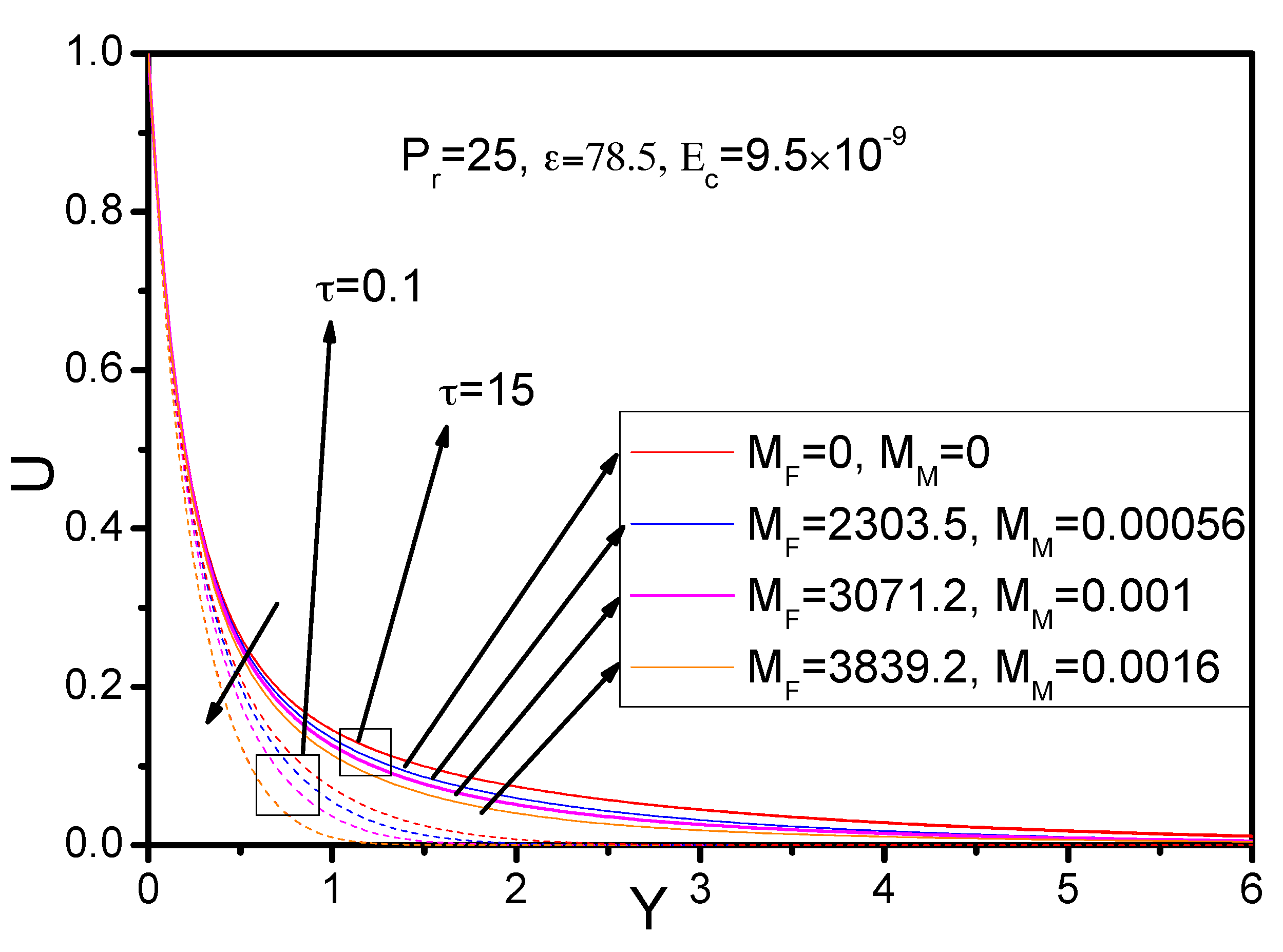
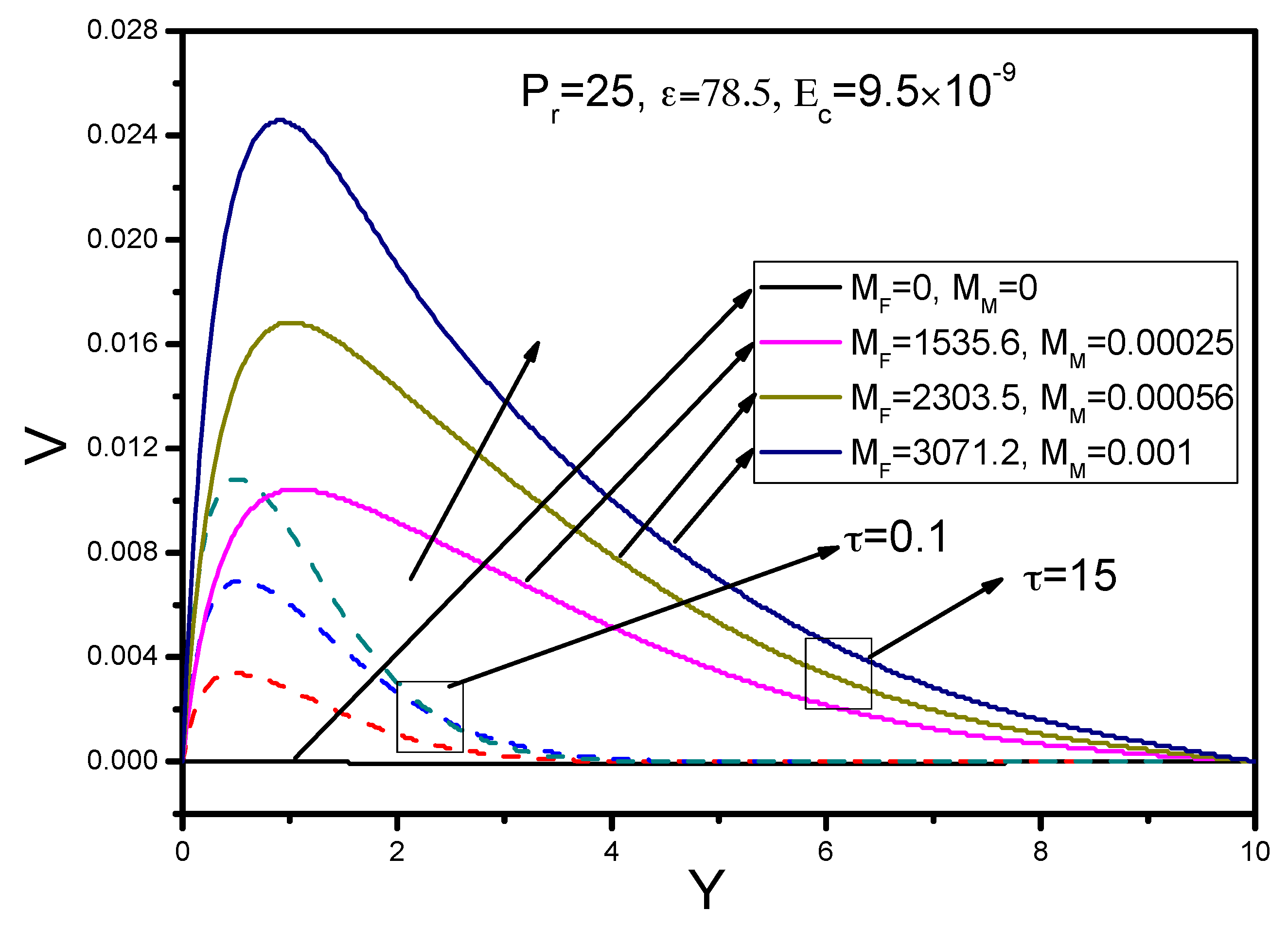
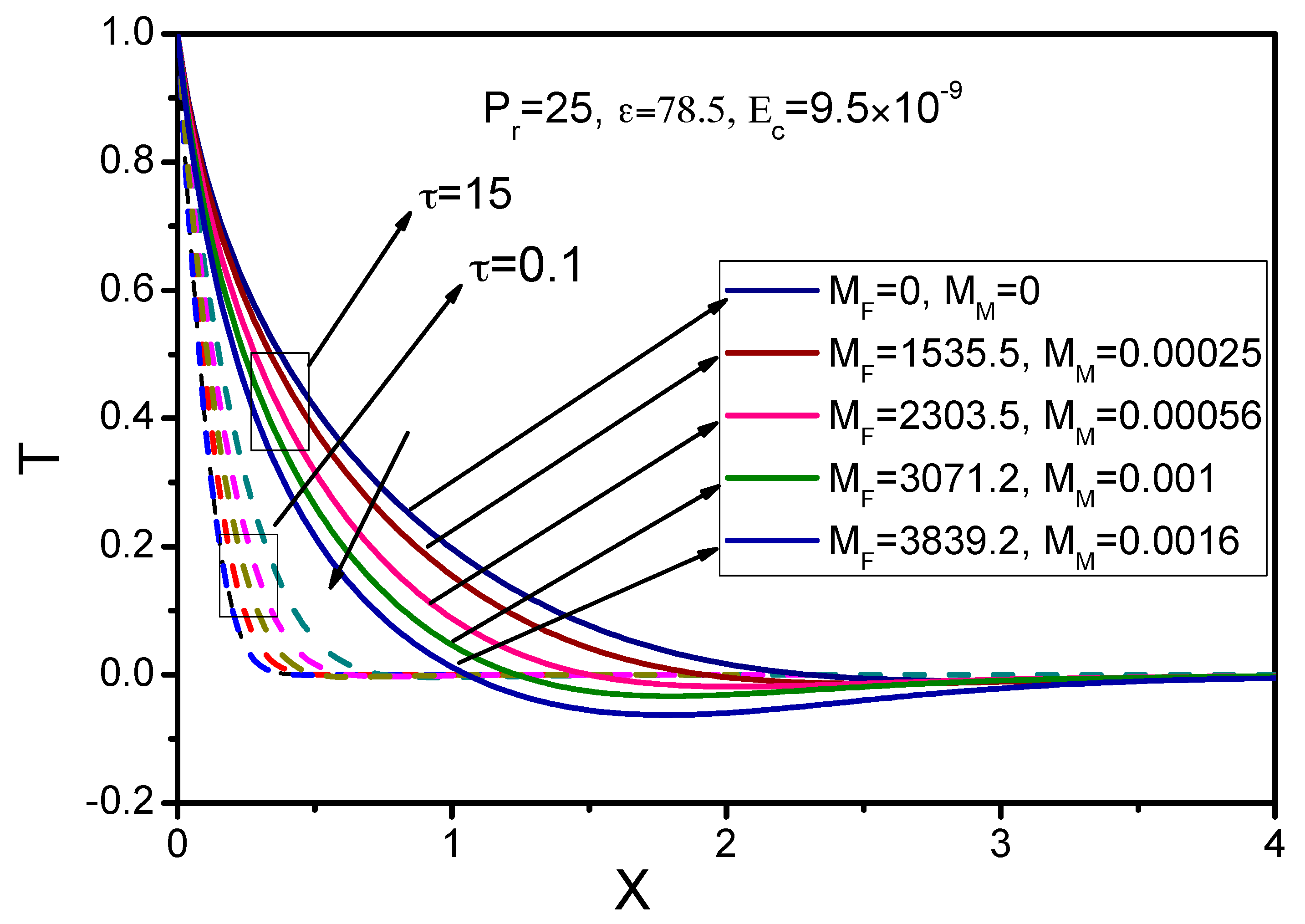
• The fluid primary velocity and temperature distribution decreased in the area of the boundary layer with the simultaneous increase of the MHD and FHD parameters, whereas the corresponding secondary velocities were increased.
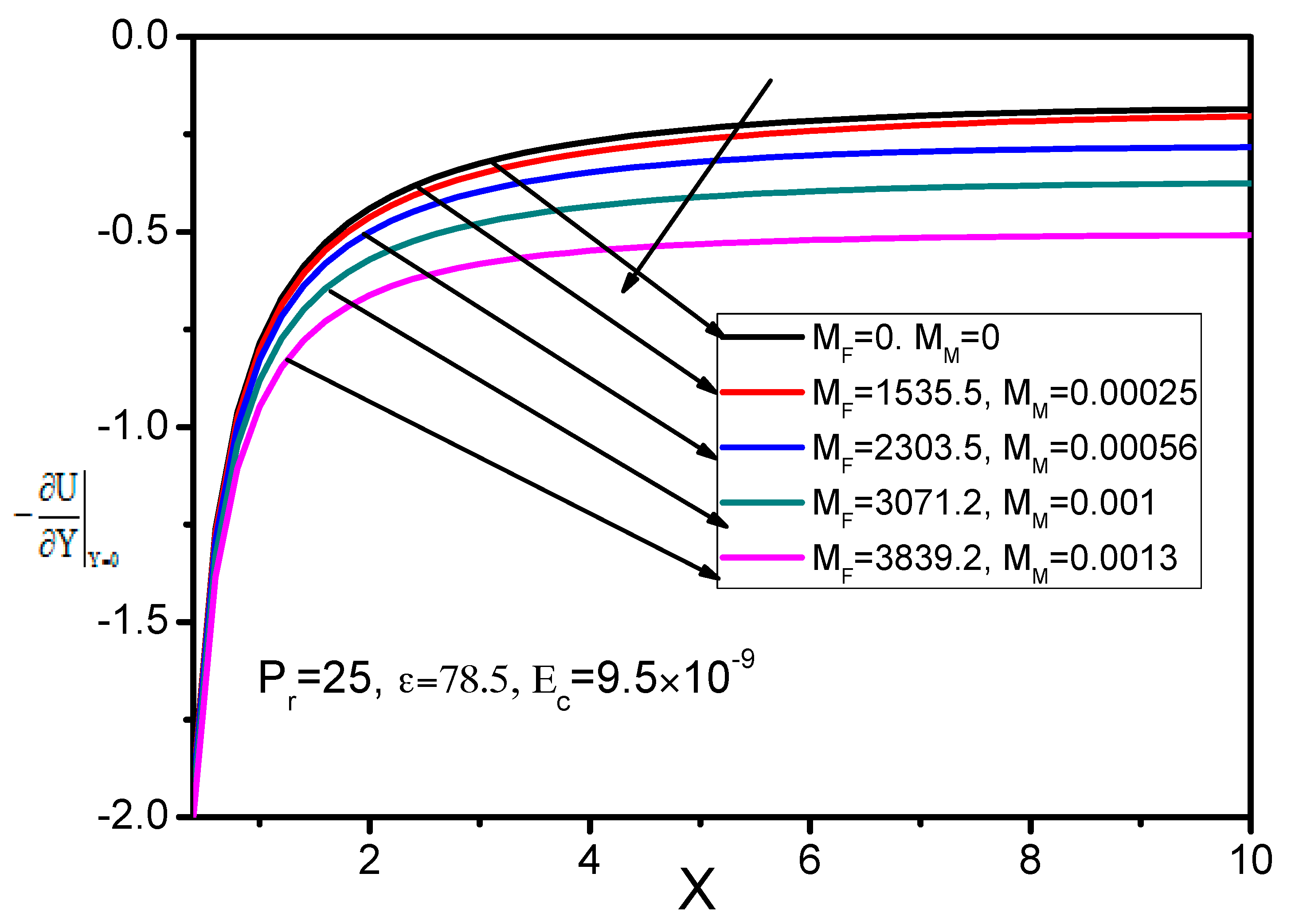
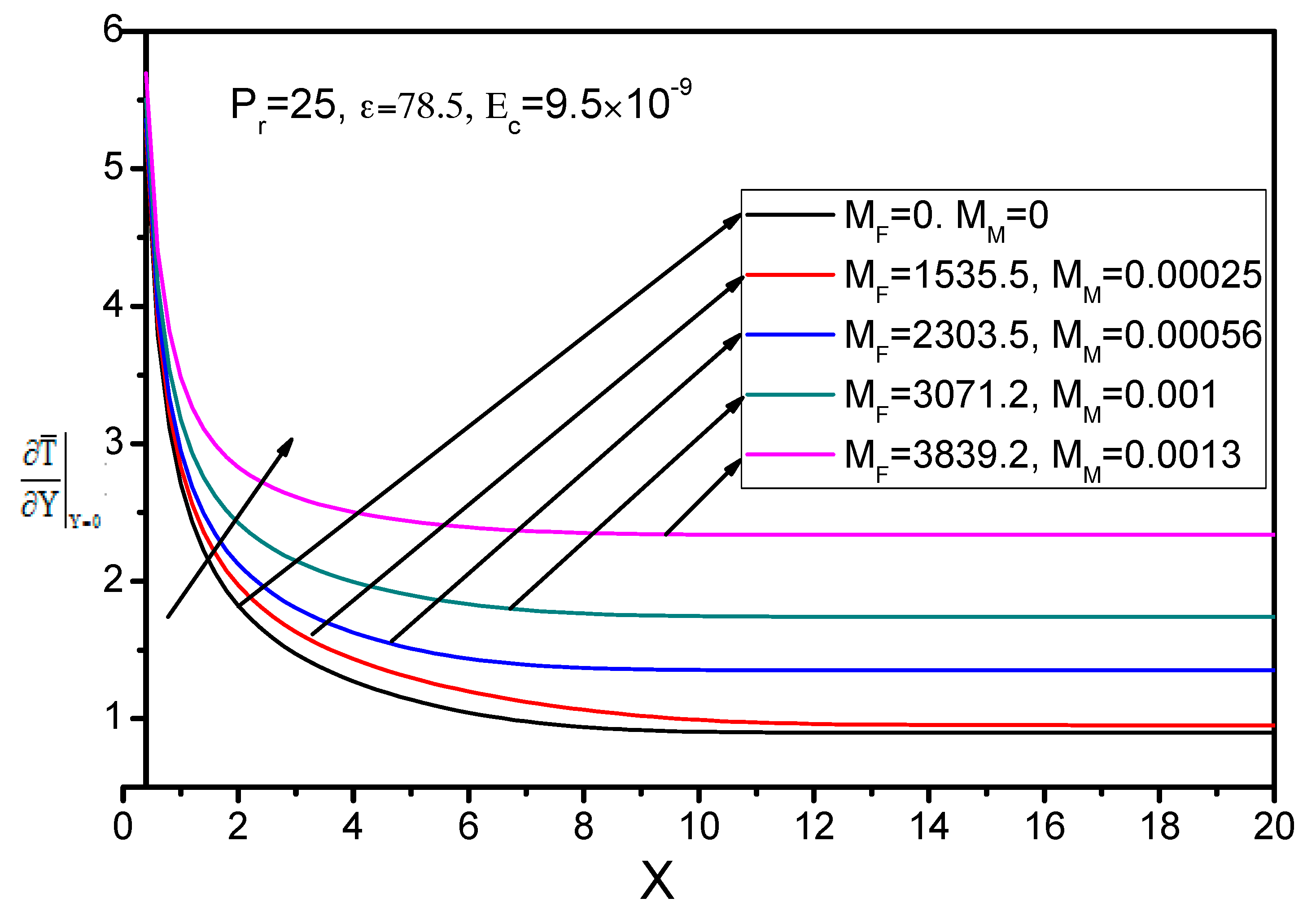
• The increment of the magnetic field resulted in a reduction of the skin friction coefficient on the wall, whereas the heat transfer on the wall was increased.
• With a greater elapsing of time $\left(\tau \right)$, the velocity and temperature profiles were found to be enhanced.

References

1. Haik, Y.; Pai, V.; Chen, C.J. Development of magnetic device for cell separation. J. Magn. Magn. Mater. 1999, 194, 261. [Google Scholar] [CrossRef]
2. Plavins, J.; Lauva, M. Study of colloidal magnetic binding erythrocytes: Prospects for cell separation. J. Magn. Magn. Mater. 1999, 122, 349. [Google Scholar] [CrossRef]
3. Voltairas, P.A.; Fotiadis, D.I.; Michalis, L.K. Hydrodynamics of magnetic drug targeting. J. Biomech. 2002, 35, 813–821. [Google Scholar] [CrossRef]
4. Ruuge, E.K.; Rusetski, A.N. Magnetic fluid as drug carries: Targeted transport of drugs by a magnetic field. J. Magn. Magn. Mater. 1993, 122, 335. [Google Scholar] [CrossRef]
5. Misra, J.C.; Sinha, A.; Shit, G.C. Flow of a biomagnetic viscoelastic fluid: Application to estimation of blood flow in arteries during electromagnetic hyperthermia, a therapeutic procedure for cancer treatment. Appl. Math. Mech. 2011, 13, 1405–1420. [Google Scholar] [CrossRef]
6. Lauva, M.; Plavins, J. Study of Colloidal Magnetite Binding Erythrocytes: Prospects for cell separation. J. Magn. Magn. Mater. 1993, 122, 349–353. [Google Scholar] [CrossRef]
7. Fiorentini, G.; Szasa, S. Hyperthermia today: Electric energy, a new opportunity in cancer treatment. J. Cancer Res. Ther. 2006, 2, 41–46. [Google Scholar] [CrossRef]
8. Haik, Y.; Chen, C.J.; Pai, V.M. Development of biomagnetic fluid dynamics. In Proceedings of the IX International SYMPOSIUM on Transport Properties in Thermal Fluid Engineering, Pacific Center of Thermal Fluid Engineering, Singapore, 25–28 June 1996; pp. 121–126. [Google Scholar]
9. Rosensweig, R.E. Ferrohydrodynamics; Cambridge University Press: Cambridge, UK, 1985. [Google Scholar]
10. Bashtovoy, V.G.; Berkovsky, B.M.; Vislovich, A.N. Introduction to Thermomechanics of Magnetic Fluids; Springer: Berlin/Heidelberg, Germany, 1988. [Google Scholar]
11. Tzirtzilakis, E.E. A mathematical model for blood flow in magnetic field. Phys. Fluids 2005, 17, 077103-15. [Google Scholar] [CrossRef]
12. Crane, L.J. Flow past a stretching plate. J. Appl. Math. Phys. 1970, 21, 645–647. [Google Scholar] [CrossRef]
13. Andersson, H.I.; Valnes, O.A. Flow of a heated ferrofluid over a stretching sheet in the presence of a magnetic dipole. Acta Mech. 1998, 128, 39–47. [Google Scholar] [CrossRef]
14. Zeeshan, A.; Majeed, A.; Ellahi, R. Effect of magnetic dipole on viscous ferro-fluid past a stretching surface with thermal radiation. J. Mol. Liq. 2016, 215, 549–554. [Google Scholar] [CrossRef]
15. Tzirtzilakis, E.E.; Kafoussias, N.G. Biomagnetic fluid flow over a stretching sheet with nonlinear temperature dependent magnetization. Z. Angew. Math. Phys. 2003, 54, 551–565. [Google Scholar]
16. Tzirtzilakis, E.E.; Tanoudis, G.B. Numerical study of Biomagnetic fluid flow over a stretching sheet with heat transfer. Int. J. Numer. Methods Heat Fluid Flow 2003, 13, 830–848. [Google Scholar] [CrossRef] [Green Version]
17. Murtaza, M.G.; Tzirtzilakis, E.E.; Ferdows, M. Effect of electrical conductivity and magnetization on the biomagnetic fluid flow over a stretching sheet. Z. Angew. Math. Phys. 2017, 68, 93. [Google Scholar] [CrossRef]
18. Ali, F.M.; Nazar, R.; Arifin, N.M.; Pop, I. MHD stagnation-point flow and heat transfer towards stretching sheet with induced magnetic field. Appl. Math. Mech. 2011, 32, 409–418. [Google Scholar] [CrossRef]
19. Misra, J.C.; Sinha, A. Effect of thermal radiation on MHD flow of blood and heat transfer in a permeable capillary in stretching motion. Heat Mass Transf. 2013, 49, 617–628. [Google Scholar] [CrossRef] [Green Version]
20. Das, S.; Chakraborty, S.; Jana, R.N.; Makinde, O.D. Entropy analysis of unsteady magneto-nanofluid flow past accelerating stretching sheet with convective boundary condition. Appl. Math. Mech. 2015, 36, 1593–1610. [Google Scholar]
21. Hayat, T.; Shafiq, A.; Alsaedi, A.; Shahzad, S.A. Unsteady MHD flow over exponentially stretching sheet with slip conditions. Appl. Math. Mech. 2016, 37, 193–208. [Google Scholar] [CrossRef]
22. Misra, J.C.; Shit, G.C.; Rath, H.J. Flow and heat transfer of a MHD viscoelastic fluid in a channel with stretching walls: Some applications to haemodynamics. Comput. Fluids 2008, 37, 1–11. [Google Scholar] [CrossRef] [Green Version]
23. Carnahan, B.; Luther, H.A.; Wilkes, J.O. Applied Numerical Methods; John Wiley and Sons: New York, NY, USA, 1969. [Google Scholar]
24. Tzirtzilakis, E.E.; Xenos, M.A. Biomagnetic fluid flow in a driven cavity. Meccanica 2013, 48, 187–200. [Google Scholar] [CrossRef]
25. Matsuki, H.; Yamasawa, K.; Murakami, K. Experimental Considerations on a new Automatic Cooling Device Using Temperature Sensitive Magnetic Fluid. IEEE Trans. Magn. 1977, 13, 1143–1145. [Google Scholar] [CrossRef]
26. Davidson, P.A. An Introduction to Magnetohydrodynamics; Cambridge University Press: Cambridge, UK, 2001. [Google Scholar]
27. Callahan, G.D.; Marner, W.J. Transient free convection with mass transfer on an isothermal vertical flat plate. Int. J. Heat Mass Transf. 1976, 19, 165–174. [Google Scholar] [CrossRef]
28. Gabriel, C.; Peyman, A.; Grant, E.H. Electrical conductivity of tissue at frequencies below 1 MHz. Phys. Med. Biol. 2009, 54, 4863–4878. [Google Scholar] [CrossRef] [PubMed]
29. Khan, M.S.; Wahiduzzaman, M.; Uddin, M.S.; Sazad, M.A.K. Finite difference solution of MHD free convection heat and mass transfer flow of a nanofluid along a stretching sheet with heat generation effects. Indian J. Theor. Phys. 2012, 60, 285–306. [Google Scholar]
Figure 1. Geometry of the flow field.
Symmetry 12 00253 g001
Figure 2. Grid of finite difference space.
Symmetry 12 00253 g002
Figure 3. Velocity profile for different grid space.
Symmetry 12 00253 g003
Figure 4. Steady case analysis for different time step.
Symmetry 12 00253 g004
Figure 5. Primary velocity for different value of MM and MF.
Symmetry 12 00253 g005
Figure 6. Secondary velocity for different value of MM and MF.
Symmetry 12 00253 g006
Figure 7. Temperature distribution for several value of MM and MF.
Symmetry 12 00253 g007
Figure 8. Variation of the skin friction coefficient for several values of MF and MM.
Symmetry 12 00253 g008
Figure 9. Variation of rate of heat transfer for several values of M F and M M
Symmetry 12 00253 g009