A Matching Pursuit Algorithm for Backtracking Regularization Based on Energy Sorting

Abstract

The signal reconstruction quality has become a critical factor in compressed sensing at present. This paper proposes a matching pursuit algorithm for backtracking regularization based on energy sorting. This algorithm uses energy sorting for secondary atom screening to delete individual wrong atoms through the regularized orthogonal matching pursuit (ROMP) algorithm backtracking. The support set is continuously updated and expanded during each iteration. While the signal energy distribution is not uniform, or the energy distribution is in an extreme state, the reconstructive performance of the ROMP algorithm becomes unstable if the maximum energy is still taken as the selection criterion. The proposed method for the regularized orthogonal matching pursuit algorithm can be adopted to improve those drawbacks in signal reconstruction due to its high reconstruction efficiency. The experimental results show that the algorithm has a proper reconstruction.

1. Introduction

Magnetic resonance (MR) image reconstruction technology has been long-established in clinical medical detection with the rapid development of medical image processing technology. It has become an essential means of medical diagnosis [1,2,3]. In practical medical applications, the traditional approach is to sample data according to the Shannon–Nyquist sampling technique. The data collected in this way can adequately represent the original signal, but they have massive amounts of redundancy. Therefore, these methods often lead to the overflow of acquisition data and the waste of sensors. It is of considerable significance to reduce the amount of data. The method of extracting a sinusoidal signal from the noise has attracted many scientists and using the compressibility of the signal to sample data is a new subject. It originates from the study of the acquisition of a finite-rate-of-innovation signal. Fixed deterministic sampling kernels are used to double the innovation rate instead of acquiring continuous signals at twice the Nyquist sampling frequency.

The compressed sensing (CS) [4,5,6,7] based on sparse representation has attracted significant attention as a new sampling theory in recent years. It breaks the limitation of Nyquist’s sampling theorem, compresses signal sampling simultaneously, saves a lot of time and storage space, and has become a new research direction in the field of signal processing [8,9,10]. CS theory has been widely used in many biomedical imaging systems and physical imaging systems, such as computed tomography, ultrasound medical imaging, and single-pixel camera imaging. Compressed sensing magnetic resonance imaging (CS-MRI) based on CS can reconstruct high-quality MR images through a small amount of sample data, which significantly shortens the scanning time, speeds up the processing of MR images, and improves work efficiency. The compressed sensing mainly includes two aspects: the first is the sampling and compression of the signal, and the second is the reconstruction of the original signal. The former is for sparse or compressible high-dimensional signals to acquire low dimensional measurement values through a measurement matrix. At the same time, the latter uses these low dimensional measurement data to restore the original signal as much as possible. However, how to design a recovery algorithm with fewer observation times, excellent reconstruction performance, and low complexity are essential challenges in the study of CS.

The basic pursuit manner [11,12,13,14] has been put forward by some scholars for this problem. The convex optimization process has a good reconstruction effect, but it is often disadvantageous to practical applications because it takes an excessively long time to run. For this reason, the greedy iterative algorithm [15,16,17,18] has been favored by the vast majority of researchers because of its low complexity and simple geometric principle. Among all the kinds of reconstruction algorithms studied at present, the greedy algorithm is the most widely used. However, in greedy algorithms, more attention is paid to a sparse unknown reconstruction algorithm, which does not need the precondition of known signal sparseness. The representative algorithms are the sparsity adaptive matching pursuit and the regularized adaptive matching pursuit algorithms. They approximate sparsity by setting an initial step and expanding the support set step by step, while the backtracking adaptive orthogonal matching pursuit uses backtracking detection to reconstruct the unknown sparseness signal. In recent years, a forward–backward pursuit (forward–backward pursuit) algorithm was proposed to estimate sparsity by iteratively accumulating the difference between the front and back steps.

An energy-based adaptive matching pursuit algorithm increases the sparsity level gradually according to the increase of the iteration residual energy. Furthermore, the adaptive matching-pursuit-based difference reconstruction algorithm uses the rate of change between the measurement matrix and the residual inner product elements to approximate the sparsity adaptively. The proposed BRAMP algorithm is also an adaptive algorithm for compressed sensing reconstruction.

The orthogonal matching pursuit algorithm (OMP) [19,20,21], the regularized orthogonal matching pursuit algorithm (ROMP) [22,23], uses each atom and the residual value of the measurement matrix for the inner product. Then, the atom that is most matched with the residual is placed in the support set using some principles. Once the atom is selected, it will not be deleted until the end of the iteration. The other is a class of compressive sampling matching pursuit algorithm (CoSaMP) [24,25], the subspace tracking algorithm (SP) [26,27]. After selecting the matched atoms, they added a backtracking function to delete unstable atoms to better guarantee the quality of the reconstructed signal. The OMP algorithm continues the principle of atom selection in a matching pursuit algorithm. Although the signal can be accurately reconstructed with only one atom being selected in each iteration, the efficiency of the algorithm is low. The ROMP algorithm, stagewise orthogonal matching pursuit algorithm, and generalized orthogonal matching pursuit algorithm can select more than one atom in each iteration, which speeds up the convergence of the algorithm. However, they cannot guarantee that the selected atoms in each iteration are correct. If the wrong atoms are selected in the previous iteration, the choice of atoms in the next iteration will be affected. The CoSaMP algorithm and the SP algorithm can select more than one atom at each iteration.

Meanwhile, the backtracking procedure is introduced to improve the reconstruction accuracy. The above algorithms increase the number of atoms to candidate sets to improve the performance of the algorithm. Due to the influence of noise observation, the performance of reconstructing signals by the above algorithms is not ideal. A regularized orthogonal matching pursuit algorithm uses regularization criteria as atomic screening rules. It can ensure that the energy of selected atoms is much larger than that of non-selected atoms, and its reconstruction performance is better than other greedy algorithms.

In this research, the regularization method was adopted to select the atomic advantage effectively, and the ROMP and SP algorithms were used to screen the atomic backtracking strategy. Further, a matching pursuit algorithm for regular backtracking based on the energy ranking (ESBRMP) was proposed. The experimental results show that this algorithm had a better reconstruction effect.

2. Compressed Sensing Theory

Let $x$ be the $N$ length of the original signal, $y$ is the $M$ length of the observed signal, ${\Phi }_{M\times N}(M<N)$ is the measurement matrix, and they meet with $y=\Phi x$. If $x$ includes $K$ sparse signals and $M\ge K\times \lg (N)$ between $K$, $M$, and $N$, $x$ could achieve the accurate reconstruction. The problem to be solved in this paper is how to reconstruct the signal $x$ from the observed signal $y$, which is usually solved using the following optimization problem:

$$\min {\Vert x\Vert }_0,\hspace{1em}s.t.\hspace{1em}y=\Phi x.$$

(1)

In practice, a certain degree of error is allowed. Therefore, the original optimization problem can be transformed into a simpler approximate solution. $\delta$ is a minimal constant:

$$\min {\Vert x\Vert }_0,\hspace{1em}s.t. {\Vert y-\Phi x\Vert }_2^2\le \delta .$$

(2)

The minimum norm problem is an NP difficult problem, and it is challenging to solve the problem directly. The matching pursuit algorithm provides a powerful tool for the approximate solution, and Tropp and Gilbert [18] pointed out that the methods for sparse signal reconstruction have a specific stability. Furthermore, the OMP algorithm continues the selection rule of atoms in the matching pursuit algorithm and realizes the orthogonalization of the selected atom set recursively to ensure the optimization of the iteration, thus reducing the number of iterations. Needell and Vershynin [22], based on the OMP algorithm, proposed the ROMP algorithm, where the regularization process is used in the OMP algorithm for a known sparsity. The difference between the ROMP algorithm and the OMP algorithm is that, first, the algorithm selects multiple atoms as a candidate set based on the relevant principles, and second, some atoms are selected by the regularization principle from the candidate set, and then incorporated into the final support set to realize the rapid and effective selection of the atom. The SP and CoSaMP algorithms use the idea of back-stepping filtering. The reconstruction quality and the reconstruction complexity of these algorithms are similar to that of linear programming (LP).

3. Reconstruction Processes

The ROMP algorithm can accurately reconstruct all the matrices and all sparse signals that satisfy the restricted isometry property (RIP) [28], and the reconstruction speed is fast. The ROMP algorithm first selects the atoms according to the correlation principle and calculates the correlation coefficient by calculating the absolute value of the inner product between the residual and each atom in the measurement matrix $\Phi$:

$$u=\left\{u_j|u_j=\left|<r,{\varphi }_j>\right|,j=1,2,3\cdots ,N\right\}.$$

(3)

The ROMP algorithm uses the regularization process to carry out the two filters of the atom. Through Equation (4), the correlation coefficients of the atoms corresponding to the index value set are divided into several groups. That is, the correlation coefficient of the atom corresponding to the medium index is divided into several groups according to Equation (4):

$$\left|u(i)\right|\le 2\left|u(j)\right|,\hspace{1em}i,j\in J_0;J_0\in J$$

(4)

The key to the regularization process is to select a set of atomic index values corresponding to the most significant energy correlation coefficients from the perception matrix, store them in the updated support set, and complete the secondary selection. Then, the atomic index value corresponding to a group of correlation coefficients with the maximum energy is deposited into $J_0$. 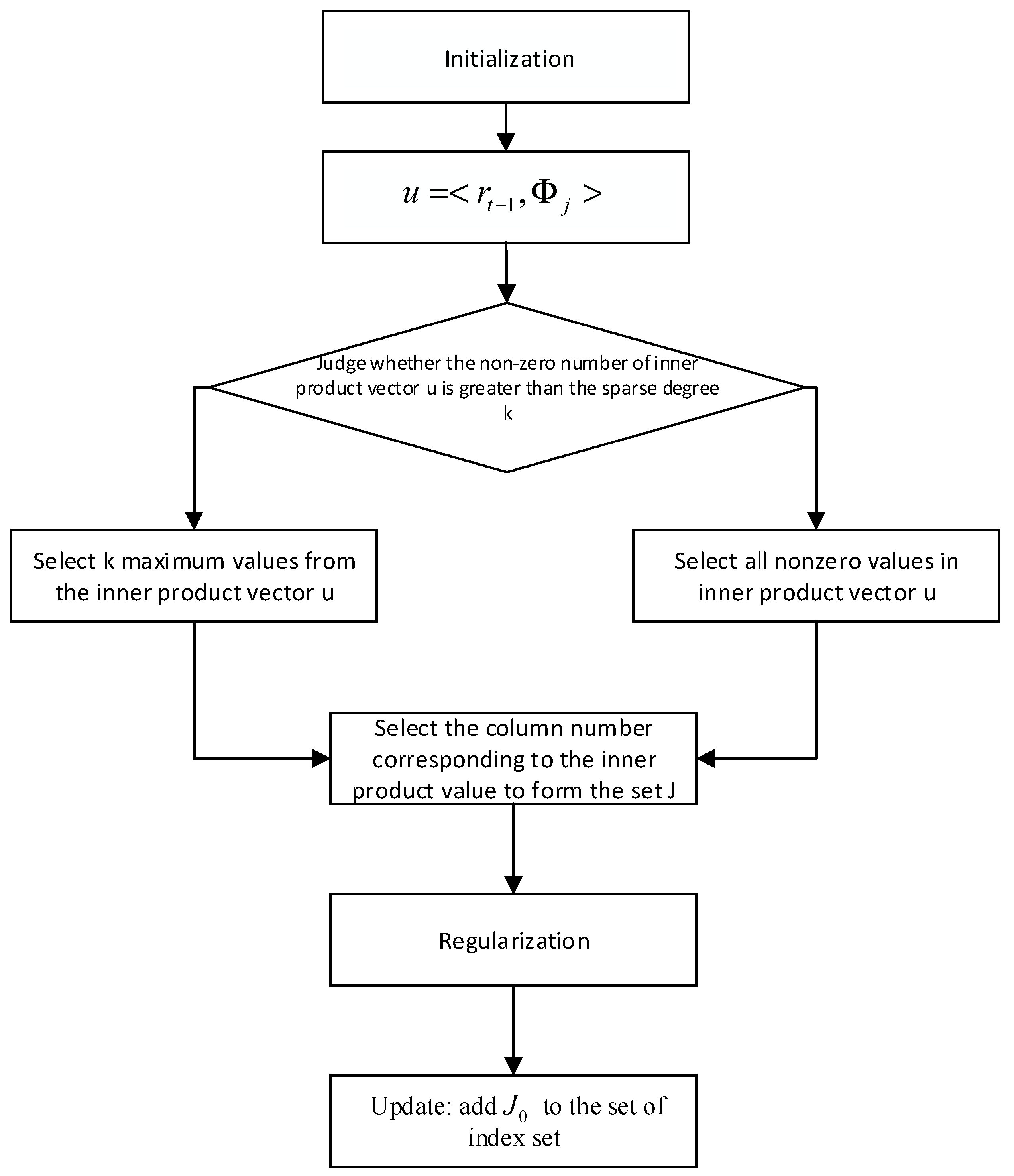The regularization process allows the ROMP algorithm to obtain the support set $|\Lambda |$ with a lower atomic number than ${\Phi }_{\Lambda }$ to reconstruct the signal accurately for most iterations. For the atoms that have not been selected into the support set, the regularization process can ensure that their energy is much smaller than the energy of the selected atoms, which is a simple and effective way of undertaking atomic screening. It could improve the stability of the signal reconstruction. After a particular iteration to get the support set for the reconstruction of the signal, the least squares method is used for the signal approximation and the remainder update. The flow chart of the ROMP algorithm is shown in Figure 1. It can be expressed as:

$$\widehat{x}=\arg \hspace{0.17em}\min {\Vert y-{\Phi }_{\Lambda }x\Vert }_2,$$

(5)

$$r_{new}=y-{\Phi }_{\Lambda }\widehat{x}.$$

(6)

The ROMP algorithm is represented as follows:

(1) Initialization: $r_0=y$, $\Lambda =\varphi$, iterating $t=1$, repeating the following steps $K$ times or until $|\Lambda |\ge 2K$.

(2) Calculation: $u=<r_{t-1},{\Phi }_j>$.

(3) The set of the largest non-zero coordinates of $K$ or all its non-zero coordinates, and the small one is set to $J$.

(4) Regularization: In all subsets with comparable coordinates $J_0\in J$, where $\left|u(i)\right|\le 2\left|u(j)\right|, i,j\in J_0{J}_0\in J$, select the maximum energy for reconstructing the original signal.

(5) Update: Add $J_0$ to the index set $\Lambda =\Lambda \cup J_0$, $x=\arg \min {\Vert y={\Phi }_{\Lambda }x\Vert }_2$, $r=y-\Phi x$.

The ROMP algorithm selects the atom through a regularization criterion in a reasonable condition. When the signal energy distribution is uniform or showing the distribution of an extreme energy state, i.e., the maximum total energy as the selection criteria, the algorithm may not accurately choose the required columns, and therefore the ROMP algorithm performance becomes unstable. The ROMP algorithm for energy sorting is proposed to solve the unstable problem, which is combined with the advantages of the ROMP algorithm and the SP algorithm. For the selection principle, first, a screening is carried out using the correlation criterion to select the column vector with the maximum inner product of the column and the iterative error vector. Then, the set of column vectors with the energy ratio less than two is selected in the selected column vector based on the regularization criterion. Lastly, the algorithm selects the set of columns that meet the requirements in all the column sets through the energy screening criteria.

The steps of the energy sorting are as follows:

(1) The correlation criterion and regularization standard selects a set of all columns: ${\Sigma }_i$, $i=1,2,3,\cdots L$.

(2) For the ${\Sigma }_i$ set of all columns, the energy $E_i$, the number of column vectors $Nu{m}_i$, and the energy average $Ev{e}_i$ are counted, where $i=1,2,3,\cdots L$.

(3) Select the maximum $n$ energy set $E_j$ by setting the energy threshold, $j=1,2,\cdots n$.

(4) Select a column $E_l$ from $E_j$ that is lower than the threshold.

(5) Find the descending order of $E_l$ through energy values, and select the set of energy averages not less than $k$ ($0<k<1$) times of later from the maximum energy value. This is the set of columns that are screened.

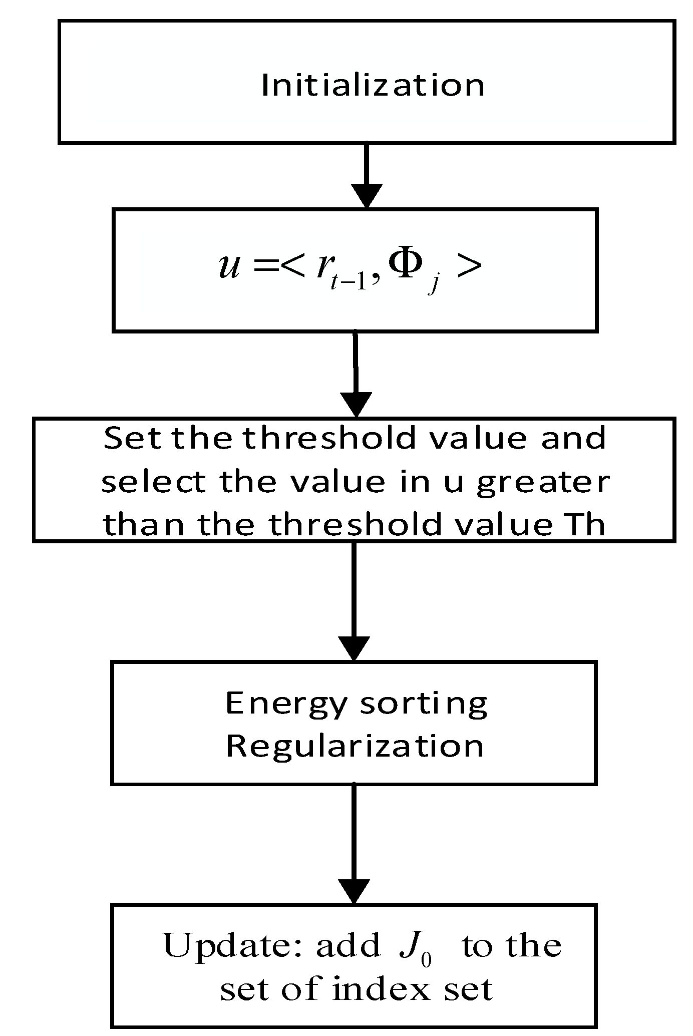
In the above steps, the purpose of step 3 is to ensure that the selected set energy is more significant than most of the sets. The purpose of steps 4 and 5 is to ensure that the selected set energy distribution is more reasonable than others. The set of columns that are filtered can contain more useful signal information. The flow chart of the ESBRMP algorithm is shown in Figure 2.

The steps of the ESBRMP algorithm are as follows:

(1)

Initialization: Set the residual $r_0=y$, $\Lambda =\varphi$.

(2)

Calculate the inner product between the residuals $r_{i-1}$ and the atoms of the observation matrix.

(3)

Set the threshold value, select the value larger than the threshold value $Th$ from $u$, and make up the set $J$ of the sequence number $j$ corresponding to these values.

(4)

Energy sorting and finding subsets $J_0\in J$.

(5)

Update the index set ${\Lambda }_i={\Lambda }_{i-1}\cup J_0$ and update the support set ${\Gamma }_i={\Gamma }_{i-1}\cup J_0$.

(6)

Solve the least squares problem $\widehat{\theta }=\arg \min \Vert y-A_t{\theta }_t\Vert$.

(7)

Backtracking update support set: Based on the backtracking idea, a new support set is made up of the larger $aL$ elements ($0<a<1$, A is the number of B)

(8)

Update the residual ${\widehat{r}}_t=y-A_t\widehat{\theta }$.

(9)

Judge whether ${\Vert {\widehat{r}}_t\Vert }_2\le {\Vert {\widehat{r}}_{t-1}\Vert }_2$ is established. If it is established, stop iterating; if it is not established, determine whether the number of initial stages s can be reached. If it is reached, the iteration is stopped; if it is not reached, return to the second step and continue to iterate.

4. Experimental Results and Discussion

The one-dimensional Gaussian random signal with an original signal length was reconstructed under different numbers of sparsity and measurement. The measurement matrix was a Gaussian random matrix. The length, sparsity, compression ratio, and the reconstruction performance of the observed signal are shown in Figure 3 and Figure 4. Figure 3 shows the ESBRMP algorithm’s reconstruction signal and residual. Figure 4 is the traditional OMP algorithm’s reconstruction signal and residual.

From the above experiments, it can be seen that the ESBRMP algorithm had a better effect on the reconstruction of the one-dimensional signal, and the residual of reconstruction was small. The related experiments were carried out on the reconfiguration rate, sparsity, and measurement of the signal, as shown in Figure 5 and Figure 6. Under different sparsities, the relationship between the measurement and the signal reconstruction rate is shown in Figure 5. When the sparsity was low, the original signal could be restored with a lower number of measurements, and the lower number of measurements produced a lower signal reconstruction rate when the sparsity was high.

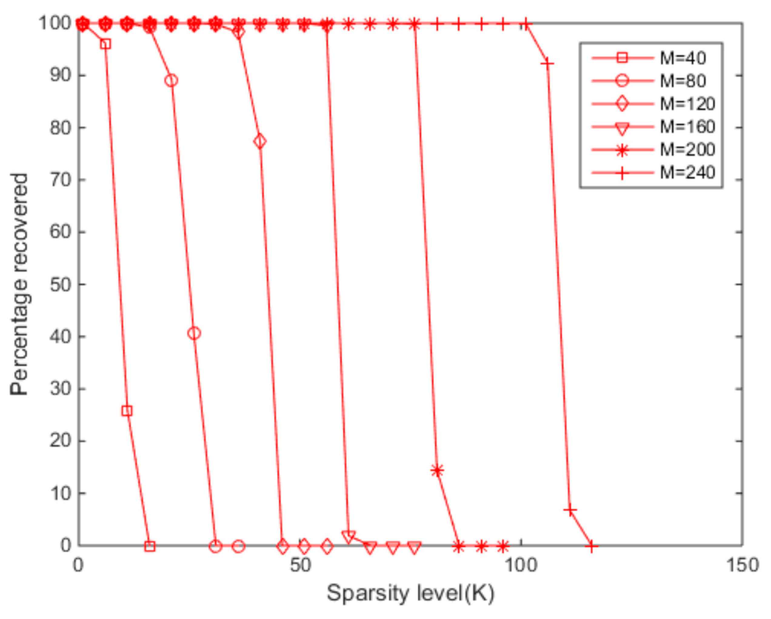
Under different numbers of measurements, the relation between the sparsity and the signal reconstruction rate is shown in Figure 6. When the number of measurements was low, the original signal could be restored with a lower sparsity, and the lower sparsity produced a lower signal reconstruction rate when the number of measurements was higher. Overall, regarding the signal reconstruction rate, the size of the sparsity was directly proportional to the number of measurements. The sparsity was more significant than usual, and the more measurements we needed to ensure that the signal had a high reconstruction rate.

The performance of the ESBRMP algorithm was compared to other typical greedy pursuit algorithms, such as the OMP, ROMP, SP, and CoSaMP algorithms. Moreover, the comparison between the exact reconstruction probability and reconstruction accuracy was verified.

The accurate reconstruction probability of the signal was compared with other algorithms. The accurate reconstruction of the signal was defined as the actual signal, which gives the same position of the non-zero elements in the recovery signal in the ideal condition without noise. The accurate reconstruction rate of the signal for different measurements M is given in Figure 7 and Figure 8. From Figure 7, for all reconstruction algorithms, the exact reconstruction probability of the first signal increased with the increase of the number of measurements M. For this algorithm, when the number of measurements was more significant than 35, the reconstruction probability of the ESBRMP algorithm was close to 1. When the number of measurements was greater than 25, the reconstruction probability of the ESBRMP algorithm was more than the OMP, ROMP, and SP algorithms. Overall, for the same signal, the number of measurements required to stabilize the reconstructed signal using the ESBRMP algorithm was less than the OMP, ROMP, and SP algorithms.

When the sparsity is greater than 60 in Figure 8, the reconstruction probability was close to 0. When the number of measurements was between 25 and 60, the reconstruction probability of the ESBRMP algorithm was higher than the other algorithms. Overall, for the same signal, the sparsity required to stabilize the reconstructed signal using the ESBRMP algorithm was higher than the other algorithms. The accurate reconstruction rate of all kinds of algorithms decreased gradually with the increase of sparsity, which was because the amount of information contained in the signal was related to the sparsity K of the signal. The sparsity K was more extensive than others, which meant there was more meaningful information. In the signal reconstruction, the atoms contained in the observation matrix were determined. More atoms were needed for the reconstruction of the signal with a larger sparsity K, while the number of atoms needed to satisfy the dictionary, the possibility of representing the signal, and the precision reconstruction rate was lower than others. On the contrary, for signals with a smaller sparsity K, the number of atoms used to represent the reconstruction was smaller. Moreover, there were many kinds of atom combinations satisfied in the dictionary, which made it possible to represent the signal and it had a higher precision reconstruction rate.

In order to further illustrate the performance of the ESBRMP algorithm, Lena images with the size of 256 × 256 were selected to compare the peak signal to noise ratio (PSNR) and the reconstruction time of the reconstructed images. First, an orthogonal wavelet transform (coif3) was used for the transform, then each column of the transformed matrix was reconstructed, and finally, the reconstructed image was obtained using the inverse wavelet transform. The measurement matrix was an orthogonal observation matrix.

Table 1. Qualities of images reconstructed and running time by different algorithms. PSNR: Peak signal to noise ratio.

Algorithms	M/N = 0.3		M/N = 0.4		M/N = 0.5
	PSNR (dB)	T (s)	PSNR (dB)	T (s)	PSNR (dB)	T (s)
OMP	23.7848	16.3249	26.3581	35.4372	29.6349	62.9146
ROMP	19.3325	2.8873	22.6383	3.0273	26.8823	3.5338
CoSaMP	22.1336	4.1558	24.0518	6.3511	25.8473	9.2915
ESBRMP	26.2538	3.2903	28.6912	5.1083	31.2703	8.9474

compares the average PSNR and reconstruction time of the reconstructed images with different compression ratios. Under the same conditions, the larger the PSNR, the higher the quality of the reconstructed images.

From Table 1, it can be seen that the PSNR value of the reconstructed image of the ESBRMP algorithm was higher than that of other algorithms, and even in the case of a low sampling rate, it still had a better reconstruction effect. The reconstruction time of the ESBRMP algorithm was higher than the ROMP algorithm and less than the other algorithms.

Table 2. PSNR of the different images using different algorithms.

Algorithms	Lena	Fruits	Cameraman	Pepers
OMP	29.6349	30.9803	28.0214	29.1471
ROMP	26.8921	28.8023	24.0257	25.7125
CoSaMP	25.8473	27.2755	24.1903	25.0361
ESBRMP	31.2703	33.4108	29.1827	30.5297

shows the reconstruction effects of different images at the same sampling rate. It can still be seen that the ESBRMP algorithm also had a strong reconstruction ability and reasonable reconstruction time for other images, which shows that the ESBRMP algorithm had better applicability than others.

The reconstruction time was related to the number of atoms needed for the signal reconstruction; the more atoms used for reconstruction, the longer the reconstruction time. Through the analysis of the accurate reconstruction rate of signal reconstruction, the results show that the larger the signal sparsity, the more atoms that were needed, and the longer the reconstruction time. On the contrary, the smaller the signal sparsity, the fewer atoms that were needed, and the shorter the reconstruction time. The reconstruction probability of the ESBRMP algorithm in the environment without noise was more than for the OMP, ROMP, and SP algorithms, and had a high probability of signal reconstruction.

5. Conclusions

In this paper, a matching pursuit algorithm for backtracking regularization based on energy sorting (ESBRMP) was proposed. The algorithm uses energy sorting to carry out two atomic screening and uses backtracking to delete individual unreliable atoms. Experimental results showed that the ESBRMP algorithm could reconstruct sparse signals with a high probability and had a high reconstruction accuracy without a noisy environment.