Crowd Simulation with Arrival Time Constraints

Abstract

Finding collision-free paths for crowd simulation has been a core technique in video games and the film industry; it has drawn a great deal of attention from computer animation researchers for several decades. Additionally, theoretical modeling of pedestrian has been a hot topic in physics as well because it allows us to predict any architectural failure of buildings and many city planning problems. However, the existing studies for path planning cannot guarantee the arrival order, which is critical in many cases, such as arrival symmetry of the characters within video games or films. To resolve this issue, a path planning algorithm has been developed with a novel method for satisfying the arrival-order constraints. The time constraint we suggest is the temporal duration for each character, specifying the order in which they arrive at their target positions. In addition to the algorithm that guarantees the arrival order of objects, a new user interface is suggested for setting up the arrival order. Through several experiments, the proposed algorithm was verified, and can successfully find collision-free paths, while satisfying the time constraint set by the new user interface. Given the available literature, the suggested algorithm and the interface are the first that support arrival order, and their usability is proven by user studies.

1. Introduction

Crowd simulation has been one of the core techniques in many industries including entertainment, transportation and architecture for many years. Particularly, computer games and feature films have many scenes where numerous agents move together. To create those crowd scenes, we need a technique to obtain collision-free paths for each individual. Various approaches have been proposed till now, under the category of multi-agent path planning techniques. One of the most popular methods is the velocity obstacles (VO) method. It can predict where the other moving objects might be in the future within the pre-defined time duration by extrapolating their velocities; hence, collisions are avoided accordingly [1]. These methods formulate a set of collision regions in the velocity domain from all neighboring characters and static obstacles at each time frame and use an optimization technique to find an optimal velocity that is as close as possible to the preferred velocity and does not intersect with the collision region. This continuous optimal speed selection creates collision-free paths for every individual. Extensions of the original idea have been proposed, such as HRVO (hybrid reciprocal velocity obstacle) [2], ORCA (optimal reciprocal collision avoidance) [3], and AVO (acceleration velocity obstacle) [4], which have their own advantages and disadvantages. Because these methods can produce collision-free paths for many three-dimensional (3D) characters successfully, they have been integrated into current commercial game engines, such as Unity or Unreal.

However, in many cases, collision-free paths alone do not suffice. If game designers or movie directors were able to control crowds so that they arrive at a particular position in a particular order, it would be possible to express various effects. For example, an entire crowd can be moved from an initial position to a target position at the same time, and could be made to engage with enemies. However, none of the previous studies [2,3,4] consider these critical time constraints when simulating multi-agents. Instead, they are concerned with ensuring that no collisions occur while the agents move to their target positions. In this study, we try to obtain the collision-free paths for crowds, subject to arrival-time constraints. Since we assume that agents have zero knowledge about the environment, they do not know how long it takes to get to the intended position. Therefore, it is very difficult to set the absolute arrival time. Instead, our algorithm focuses on the relative time difference among the agents’ arrivals. This would give the arrival-order constraints over the crowds. For example, all agents could be made to arrive at their intended position simultaneously, or given an initial line formation, we can make them arrive at their target positions from left to right. As another example, we can make moving objects symmetrically arrive at the targeted positions at the video games, or the films. Furthermore, we can control the arrival times of drones to give more impressive effects to attendances. In summary, supporting the relative arrival times of objects to specific positions can further increase the controllability of objects.

To solve the ordered arrival-time constraint, this study proposes algorithms featuring three main contributions. First, to meet the time constraints, we put a velocity-adjustment layer on top of the existing ORCA method. This layer adjusts the velocities of all agents so that they arrive at their target positions in a particular order. Whereas the original ORCA method has a fixed range of speed, the proposed method allows the maximum speed parameter to change, to meet the time constraints. Although the original ORCA algorithm creates collision-free paths for multiple agents, it cannot be used to control their relative arrival times. That is, it cannot control the order in which the agents arrive. However, the proposed methods not only produce the collision-free paths, but also satisfy the arrival-time constraints.

Second, to find a set of waypoints for a highly complicated environment, a modified PRM (probabilistic roadmap) method is proposed, which can reduce the potential future collisions for multiple agents. The modification scatters the shared waypoints of multiple agents slightly so that the agents can have different waypoints; this has the effect of reducing future collisions.

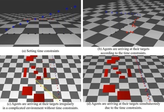
Third, a novel user interface is proposed for setting the time constraints. Usually, the timeline interface has been widely used for time-domain multimedia applications. However, it is not efficient for multi-agent simulation because a timeline must be given for each agent. If hundreds of agents are to be simulated, then the same number of timelines must be created, which is not easy to control. The novel interface instead integrates the time constraints with the environment. Specifically, it is assumed that the y-axis (up vector) of the environment is a time domain. When the target position of each agent is set up, another time point is allowed for setting their arrival time. The farther the point is from the ground, the later the agent arrives at the goal. A key point is that the time point does not represent the absolute time of arrival. Instead, the gap between two time points is of significance, as it represents the time difference between two arrival times. Through a series of experiments, it was verified that the proposed algorithm could exactly create paths for many agents satisfying diverse time constraints in real-time. Furthermore, a new user interface is proposed that can be used to set constraints around 30 percent faster than the timeline interface.

The remainder of this paper is organized as follows: Section 2 lists and overviews all the related work. Section 3 illustrates the proposed algorithm in detail. In Section 4, we show experimental results, including performance graphs. Finally, Section 5 concludes the paper with discussion and future work. In this paper, the terms “crowds” and “multi-agents” are used interchangeably.

2. Related Work

For the past few decades, crowd simulation has been one of the more active research areas in the computer animation research community, and many different approaches have been proposed [5]. Excellent module-based software architecture for pedestrians, including motion synthesis and path planning has also been proposed [6]. Crowd simulation techniques can be divided into two categories: macroscopic models and microscopic models [7,8,9]. Macroscopic models usually view the entire crowd as a single group and focus on the natural flow of crowd movement. Continuum crowds and aggregate dynamics [10] are two popular macroscopic crowd simulation models. As these approaches do not factor in individual behavior, detailed quality of motion in simulation is not their top priority. Recently, Karamouzas et al. analyzed a large corpus of real crowd data and found that interaction energy between two pedestrians follows a power law as a function of their projected time to collision [11]. Using this law, they were able to simulate a more realistic flow of movement, including the self-forming lane phenomena. They further proposed an implicit crowd simulation [12] method. This method was based on an energy-based formulation in a physics-based simulation. To update the agent’s position, they proposed an optimization-based integration scheme. In their formula, the entire crowd was considered to solve the optimization; this made it hard to implement the method for large crowds in real-time, although the overall movement of crowds was quite realistic.

Conversely, microscopic models focus on individual behaviors and interactions between agents. The classical social force model and Boids model [13,14] are two widely used models, for simulating flocks based on interactions between individuals. Another algorithm integrates the popular A* path planning with crowd density information so that agents could avoid high-density areas when they plan a path [15]. In [16], the algorithm applies PLE (principle of least effort), a general principle of crowds, to find a biomechanically energy-efficient collision-free trajectory by performing an optimization on the total amount of metabolic energy used when traveling to the goal.

Some other methods have been proposed for multi-agent path planning to meet constraints. For example, the MAPF-POST (multi-agent path finding) algorithm suggested in [17] took into account kinematic constraints such as the maximum translational and rotational velocities of agents, and built a simple temporal network to post-process the output of an MAPF solver using artificial intelligence (AI) to create a plan-execution schedule. This method is similar to our proposed method, in that both methods targets creating collision-free paths for a multi-agent system, while satisfying constraints. However, the constraints in [17] include only kinematic constraints. The proposed study aims to solve the problem of temporal constraints, which gives more controllability to the agents.

The proposed method solves the time constraint problem by augmenting a new functional layer that adjusts velocities to meet the given time constraints on the existing velocity-based models. Among the velocity-based models, ORCA (optimal reciprocal collision avoidance) has an advantage in obtaining a collision-free path for n-body moving objects [3]. In this formulation, each agent considers a neighboring moving object and constructs a half-plane defined in velocity space that is selected to guarantee collision avoidance. The agent then keeps selecting their optimal velocity from the intersection of all half-planes, which can be done efficiently using a simple optimization technique [3]. This method enables agents to avoid collisions while they are moving to their respective target positions. However, there are still some cases when they get stuck, and it takes time to extract themselves from the situation. In addition, the original ORCA method does not focus on how long it takes for agents to arrive at the target positions. Instead, it only emphasizes obtaining only collision-free paths. The proposed method modified the existing ORCA to satisfy time constraints. First, the algorithm checks the visibility to the current waypoint, all the time. If the waypoint is visible, it uses the time-constrained maximum speed parameter rather than the fixed one, which can expand the range of speeds, to support constrained arrival times. Second, once the ORCA decides the collision-free final velocity through the optimization process, the algorithm adjusts it automatically to meet the time duration constraints.

Meanwhile, the robotics research community has been working on computing collision-free, feasible motion paths for an object from a given starting position to a given target, in a complicated workspace. To this end, the probabilistic roadmap (PRM) approach is a commonly used motion planning technique [18]. The core part of this approach is a sampling method that samples the configuration space of the moving objects. In a simple two-dimensional (2D) environment where agents are moving on a flat ground, the sampling involves obtaining a set of 2D points distributed in the environment that do not collide with static obstacles. Further, those 2D points are connected to generate a roadmap. The roadmap is then used as a set of waypoints to find a path. To find a path for the given initial and target points, the Dijkstra algorithm is applied on the roadmap [19]. One of the problems of the method is that it is not made for multi-agents. Although the method can produce a path in a highly complicated environment where a lot of obstacles exist, for a finite number of samples, if the initial and final positions of two agents are similar, then there is a high probability that these two agents keep colliding during the simulation. To solve this problem, a method is proposed to perturb waypoints in the paths so that the agents have slightly different waypoints in their respective paths; this can reduce the possibility of collision.

In terms of setting time constraints, the timeline interface has been used for multimedia-related authoring tools [20]. In the timeline interface, a horizontal bar represents an event in the time domain. Users can put a marker on the bars, cut them out or concatenate them together. This is quite efficient for a simple time-related manipulation task. However, it is not efficient for crowd simulation, because a timeline must be created for each agent. As the number of individuals increases, the number of timelines must increase as well. In this paper, the timeline interface is integrated with the environment directly. Through this interface, users can conveniently set the time duration constraints interactively. In addition, users can use a grouping tool for setting time constraints to multiple agents at the same time.

3. Proposed Algorithms

3.1. Problem Statement

The problem consists of path planning for N agents, with arrival time constraints between agent pairs. Each agent is assigned a target point, which is denoted as $G_i\in {\mathbf{R}}^2$, where $0\le i\le N$ and each G_i consists of a set of waypoints $\left\{W_j\in {\mathbf{R}}^2\right\}$ to get to the target G_i, where $0\le j\le m$. The arrival-time constraints are represented as $T_i\in R$, and ∆T_i is the difference of adjacent two T_i and their average $\widehat{T}$. Given these configurations, collision-free paths must be found for all agents such that for each agent, the difference between the actual arrival time and the estimated average arrival time, $∆A_j = \widehat{A} - A_i$ matches $∆T_i$.

3.2. Overview

The simulation follows the steps illustrated in Figure 1. In the pre-processing step within Figure 1, given a set of static obstacles, the algorithm constructs a roadmap through the PRM planning method. At run time, the user first specifies the target position and time duration constraints for all agents. Then, the waypoints are obtained through a roadmap query to the PRM. The waypoints behave like sub-goals, as the agent moves to the target. The current waypoint is set to the starting waypoint in the beginning, and moves to the next waypoint as the agent passes by. The preferred velocity can be computed from the current waypoint and the agent’s position. Further, the visibility is checked to see if there are any obstacles up to the current waypoint. If there is no obstacle, then the maximum speed parameter is adjusted so that the agent can move through the current waypoint, while satisfying the time constraints.

As illustrated in [3], given the preferred velocity and maximum speed parameter, the algorithm constructs a set of ORCA half-planes from neighboring agents and static obstacles, and applies linear programming to obtain the optimal velocity. At the final step, the optimal velocity is adjusted again to satisfy the time duration constraint. Once the final velocity is computed, an Euler integration is applied to update the agents’ positions.

3.3. Pre-Processing Step

This section explains the roadmap construction using the PRM method. To navigate through the highly complicated environment where many static obstacles exist, the agents must have a rough picture of the paths that they move along. For this purpose, the algorithm constructs a roadmap that guides agents to the target positions. There are many sophisticated high-level motion planning algorithms available in robotics research, including PRM, RRT (rapidly-exploring random tree), and others [18]. Among them, we use the PRM owing to its simplicity in implementation. Figure 2 shows an example of a roadmap constructed by the PRM.

One issue of the original PRM is that it does not support multiple agents, due to which two agents can sometimes have similar paths if their initial and target positions are not separated far enough. To solve this problem, the proposed algorithm randomly perturbs the path when the two agents share the same waypoint. Assume that there are two paths P₁ and P₂ as shown in Figure 3. In Figure 3a, it happens that both P₁ and P₂ have the same waypoint w_i. In this case, if those two agents have a similar speed, then there is a high chance that the two agents would bump into each other at some point in time. To prevent this collision, the algorithm maintains an internal count variable for each waypoint. If a certain path uses a waypoint, then the count variable increases its value. If another path lies on the same waypoint, then instead of using the original waypoint, the algorithm finds a new position that is close to the original waypoint. The new position should not lie on any static obstacles and should be a within a threshold distance range from the original waypoint. Figure 3b explains the new position, perturbed from the original waypoint.

3.4. ORCA with Modified Preferred Velocity

The velocity obstacle (VO) is defined as a set of velocities that lead to a collision for moving an agent a, if the agent maintains its current velocity for a short period [1], given other dynamically moving agents playing the role of moving obstacles. In general, VO is defined in velocity space. Specifically, assume that $V{O}_a$ is a VO induced by agent a. Then, VO is constructed by translating a collision cone, a set of velocities that lead to a collision eventually, given the velocity of agent a, denoted by $v_a$. Figure 4 illustrates the VO for agent a given another agent b. Although we discuss the method only for agent a given another agent b, the method can be applied to the agent b given agent a, because the method is reciprocal.

To avoid collision, the agent should find a new optimal velocity outside VO_a. The meaning of optimal in our approach requires the input of a preferred velocity. The preferred velocity is a vector obtained by multiplying a speed parameter with a direction vector. The direction vector is defined a unit vector from the agent’s position to the current waypoint. The optimal velocity must then be chosen to stay outside of $V{O}_a$ and to be as close to the preferred velocity as possible. In our approach, rather than using fixed maximum speed $S_{max}$, it is allowed change, depending on the visibility. This approach makes the agent arrive at the waypoint a little early, which gives some extra time to adjust the velocity to meet the time constraint.

The visibility check decides if there are obstacles to the current waypoint. Clearly, all waypoints are sampled so that they are not inside static obstacles. Therefore, the visibility checking here only accounts for other moving agents in the straight line to the current waypoint assuming that current waypoint is visible from the current agent unless there are other agents in between. Mathematically, assume that we have agent $\mathit{a}$ at the position $p_a$ and their current waypoint is $w_i$. Then, if the distance $d$, the length of the perpendicular vector to $w_i-p_a$ as indicated in Figure 5, is smaller than the agent’s size $r_a$, it shows that the waypoint $w_i$ is not visible from $p_a$. Otherwise, the agent can go to the waypoint directly. The distances $d$ and $l$ are calculated by following Equations (1) and (2):

$$d=\sqrt{{\Vert \overrightarrow{p_b{p}_a}\Vert }^2-l^2}$$

(1)

$$l=\overrightarrow{p_b{p}_a}·\frac{w_i-p_a}{\Vert w_i-p_a\Vert }$$

(2)

Depending on the visibility, the preferred velocity can be calculated as follows:

$$v_a^{pref}= \{\begin{array}{cc}{S}^{*}{}_{max}\frac{w_i-p_a}{\Vert w_i-p_a\Vert }& : if visible \\ S_{max}\frac{w_i-p_a}{\Vert w_i-p_a\Vert }& : if not visible\end{array}$$

(3)

where $w_i$ is the current waypoint, $p_a$ is the current position of agent $\mathit{a}$ and $S^{*}{}_{max}=S_{max}\ast l\ast k. S_{max}^{*}$ is the modified maximum speed of the agent, which is a scalar value, where $S_{max}$ is the original maximum speed parameter and $k$ is the distance constant value, which works as a control parameter on how imminent the collisions are. The scalar $l$ represents the length of the projection of the vector $\overrightarrow{p_b{p}_a}$ on to the vector $\overrightarrow{w_i{p}_a}$. The value of $k$ controls the magnitude of $S_{max}.$

Then, the optimal velocity $v_a^{opt}$ can be defined as follows:

$$\begin{gathered} v_a^{opt}=\mathbf{arg}min\Vert v-v_a^{pref}\Vert \\ \mathrm{where} v\in \{v\in {\mathbf{R}}^2|\Vert v\Vert <S_{max}, v\notin V{O}_a\}. \end{gathered}$$

(4)

To choose an optimal velocity, it must be outside of the $V{O}_a$ and be as close to the preferred velocity as possible. The optimal velocity can be found through a mathematical optimization technique such as a linear programming [1].

The problem of the original VO is that sometimes oscillations may occur during simulation because there is no guarantee that the desired velocity chosen by the agent a lies outside the VO when another agent chooses their velocity simultaneously. To fix this issue, the algorithm is upgraded so that each agent takes half of the responsibility of avoiding collision. It is called the RVO (reciprocal velocity obstacle). To implement the RVO efficiently while minimizing unnatural movement, the ORCA algorithm was proposed [3]. The ORCA argues that the velocity obstacles, along with the so-called half-plane that contains a set of collision-free velocities, generate smooth trajectories. Let $v_a$ represent the current velocity. In ORCA, a new parameter called the finite time horizon $\tau$ is introduced. The finite time horizon $\tau$ is the period that guarantees collision-free movement, which means that future collisions are ignored beyond $\tau$. With $\tau$, the $V{O}_a$ is often truncated into $V{O}_a^{\tau }$, which would reshape the collision cone (to be rounder). Let $q$ be the nearest point on the border of $V{O}_a^{\tau }$, $u$ be the vector connecting $q$ and $v_a$, and $n$ be the outward normal vector of $q$ and $V{O}_a^{\tau }$. Then, $q$ can be calculated as follows:

$$\begin{gathered} q=\mathbf{arg}min\Vert u-v_a\Vert \\ \mathrm{where} v\notin V{O}_a^{\tau }, u=q-v_a \end{gathered}$$

(5)

To calculate the optimal vector for n neighboring agents, ORCA defines the half-plane as a plane perpendicular to $n$ at the point $v_a+\frac{1}{2}u$. Figure 6 shows the ORCA and the truncated $V{O}_a^{\tau }$. More details on ORCA algorithm can be found in [3].

3.5. Adjustment of Velocity for Time Constraints

Given arrival-time constraints, the velocity of the agent must be adjusted to satisfy the constraints. First, the algorithm calculates the arrival-time to the target of each agent. To calculate it, the total length of the path for a given set of waypoints is needed. For this, the distances between adjacent waypoints are summed. Assume that the set of waypoints for agent a is $\left\{w_i\right\}$. Then the total length of the path, $D_a$, can be calculated as follows:

$$D_a= {\displaystyle \sum }\Vert w_i-w_{i-1}\Vert$$

(6)

Since the $D_a$ does not take collision avoidance into account, the actual trajectory that the agent moves along may be different from this path. Assuming that the agent a maintains its current velocity, and that $D_a$ is the total length of the path it traverses, the estimated arrival time $A_a$ can be calculated as follows:

$$A_a=\frac{D_a}{\left(\Vert v_a\Vert + \mathsf{\epsilon }\right)} ,$$

(7)

where $v_a$ is the current velocity, and $\mathsf{\epsilon }$ is the smallest floating point value to prevent division by zero.

Since $A_a$ is estimated at every time frame, $\mathsf{\epsilon }$ is required, as sometimes the agent may not move during the simulation, which generates a zero velocity. Given the estimated value $A_a$ for agent a, the velocity can be recalculated for given time constraints $T_a$. The time constraint $T_a\in R$, is a scalar value that indicates the arrival time of agent a. The key point to note is that $T_a$ does not mean the absolute time at which the agent a arrives at the target. In the proposed simulation, the difference of this value with time constraints of other agents is of more importance. Mathematically, assume that there is a set of constraints $T_i$ where $0\le i\le n$. For example, $T_0$ is the time constraint for agent 0, $T_1$ is the time constraint for agent 1, and so on. Succinctly, the value of $T_i$ is meaningful only when it is compared with some other $T_j$. That is, if $T_i$ is smaller than $T_j,$ agent i arrives at its target position faster than agent j. The extent by which the agent i arrives before agent j depends on the difference between $T_i$ and $T_j$. For example, let three agents and their $T_i$ be 0.1, 0.5, and 0.3, respectively. Then, the order of arrival is the first, the third, and the second.

The difference between two $T_i$ is the difference in arrival times. By changing values, the arrival time can be controlled. For instance, if $T_i$ is the same for all agents, they must arrive at their targets simultaneously. For the three-agent example above, the suggested algorithm does not distinguish between the cases when all $T_i$ are 0.1, or when all $T_i$ are 0.2. To adjust the speed of agents based on $T_i$, a standard arrival-time is needed. In this approach, the standard arrival time is set as the average of $T_i$, denoted as $\widehat{T}$. Controlling the speed of particular agents, now depends on the difference between $T_i$ and $\widehat{T}.$ Similarly, the algorithm calculates the average arrival time,$\widehat{A}$, for all agents:

$$\widehat{A}=\frac{1}{n}{\displaystyle \sum }{A}_i$$

(8)

Given $\widehat{A}$ and $\widehat{T}$, the adjusted velocity $v_i^{\prime }$ can be calculated for agent i by:

$$v_i^{\prime }=\frac{(\widehat{A}-min(∆t_i,∆t_{max}))+A_i}{D_i}{\widehat{v}}_i$$

(9)

where $∆t_i=\widehat{\mathrm{T}}-T_i$, $∆t_{max}$ is the allowable maximum $∆t,$ and ${\widehat{v}}_i$ is the normalized velocity.

In the proposed algorithm, velocity is allowed to change only when the current waypoint is visible. This basic strategy is to make each agent adjust their speed as often as possible whenever the current waypoint is visible. The maximum $∆t_{max}$ is set so that $∆t_i$ cannot be larger than a threshold, which is needed to prevent an unnecessarily large arrival-time difference.

3.6. User Interface for Setting Time Constraints

To set a time constraint for a specific agent, an efficient user interface is needed. The timeline interface has been used for multimedia applications that require time-domain data. However, it is not easy to apply it for crowd simulations, where a lot of agents move together. If a timeline is to be put for each agent, the number of timelines can be too many, which needs a lot of scrolling for a given fixed window size. In the proposed approach, a simple interface is designed, integrated with the environment directly. Figure 7 shows the user interface. It is assumed that the y-axis (up vector) of the environment is the time domain. Then, the target points are duplicated into so-called time points, and each time point is allowed to move along the y-axis. The farther the time point is from the ground, the longer the corresponding agent takes to arrive. By changing this target position on the y-axis, the order of arrivals can be controlled. Simply selecting with a mouse and dragging enable control over the time points. Group selection can also be allowed so that multiple constraints can be moved up and down at the same time.

4. Experiments

A crowd simulation system was built on Microsoft Windows 10. The hardware specifications included the following: a single Intel i7 CPU with a 16 GB main memory. The graphics card was NVidia’s GeForce GTX 1060. OpenGL was used for 3D rendering. The library for the original ORCA algorithm was provided by [17]. For all the experiments in this section, the number of samples of the PRM planning was set to 1000, the perturbation value of r was set to 1.0, and the distance constant k for calculating $S^{*}{}_{max}$ in Equation (3) was set to 5.0. For the ORCA, the maximum speed $S{}_{max}$ was set to 2.0 and the agent’s size, r_i was heuristically set to 0.5. For fast neighbor searching, a simple grid-bin method was used on a KD (K-dimension) tree structure. To increase the understandability of the figures in this section, a result video was created. Please refer to the accompanying video and Supplementary Materials at online https://youtu.be/qu_sxFoRhdg.

Figure 8 shows the simulation result for 10 agents. In the first scenario, the simulation without time constraints is compared with the one with time constraints. The initial positions of agents are arranged vertically. The time constraints are set such that all agents arrive at their targets simultaneously. If the time constraints were not set, all agents would make their way to the target independently. However, when the time constraints are set, the agents adjust their velocities considering all other agents, and finally arrive at the targets at the same time. Fast-moving agents decrease their speed, and slow-moving agents increase their speed. The total amount of time taken to reach their targets is similar in both cases (13 and 12 s, respectively).

Figure 9 shows the proposed user interface for time constraints integrated with the environment. Users can adjust the relative time gap between two agents by moving the time points up and down, i.e., by conveniently dragging the mouse. In this scenario, agents were required to arrive at their target positions in the left-to-right order. The simulation result shows that the constraints are exactly satisfied. The total simulation time was around 14 s. The time difference between the first and last arrivals was around 6 s. The value of $∆t$ between two adjacent time constraints was 1.5–2.0 s.

Figure 10 shows another simulation example, where all agents formed a circle at the beginning and tried to get to the opposite target positions. The time constraints were set to make them arrive at the targets simultaneously, which is a harsh condition, as there is heavy traffic at the center. The result shows that all agents were able to solve the situation, and eventually maneuver to their targets at the same time. The total simulation time was around 24 s, which took longer than other scenarios due to the heavy traffic in the middle.

Figure 11 shows the scenario where the environment has static obstacles. The algorithm applies the modified PRM to obtain the waypoints for each agent. The arrival order was set in an arch and symmetry style so that agents gradually arrive at their targets, from the center to both ends. The result shows that the agents avoided all obstacles and made their way to their targets in a specific order. The total simulation time was around 14 s. In addition, to test the scalability of the proposed algorithm, it was tested with more agents and in more complicated environments. Figure 12 shows the simulation result of 30 agents in the environment with relatively more obstacles. To make the scenario more complex, all agents were required to arrive at their target positions simultaneously. The result shows that the proposed algorithm satisfies the arrival-time constraints for all the agents.

Figure 13 shows how the algorithm makes the agents satisfy the arrival-time constraints. The x-axis represents the particular agents and y-axis indicates the time domain. The time constraint and the actual arrival times are put in the same time domain together for comparison, although the two are conceptually different. The value of time constraints shown in blue lines indicate y, the time points of the environment, and orange lines indicate absolute arrival times. As can be seen in the figure, the two lines have almost identical shapes, meaning that the agents’ arrival times satisfy the constraints.

The graph in Figure 14 represents the performance. On the same complicated environment as in the final scenario, the number of agents were increased from 5 to 100 and the frame rate was checked. The result shows that the proposed algorithm has linear performance as the number of agents is increased, and maintains a stable real-time performance. Even when the number of agents was increased to 100, the framerate did not go below 40 frames/s, which substantiates the real-time performance. Note that the framerate takes the simulation and rendering times into account.

In summary, the proposed algorithm was tested in several scenarios. Given a set of targets, the targets were specified to the agents randomly. This setting generates a different result for each simulation. It was found that the simulation time ranges between 10–20 s, when the Euclidean distance between agent and target is around 10 units. During the simulation, no collisions were observed between the agents. This demonstrates that the proposed algorithm is reliable and has a stable real-time performance.

Since the suggested algorithm is the first for path planning with time constraints, it was compared with the A* path planning algorithm in

Table 1. Comparison between the proposed modified PRM and the A* algorithm in terms of construction time.

	Modified PRM	A*
Time	1.2 s	3.2 s

, in terms of the total amount of time taken for construction. The amount of time includes the pre-processing steps, in both cases. More details on the A* algorithm and its efficiency can be found in [21,22].

To this end, 3000 samples were used for the PRM and a grid size of 0.1 was set in the A* algorithm, in the environment of size 1000 × 1000 units. The result shows that the modified PRM is 2.6 times faster than the A* algorithm, even while supporting the time constraint that the A* algorithm does not. The speculation behind this, is that the A* algorithm requires a significant amount of time to calculate all-pair-paths. Once the pre-processing is done, actual path planning for the given initial and target positions can be done in real-time, for both cases.

To check the efficiency of the proposed user interface, a simple experiment was performed, in which 30 agents were created and the time taken to set the time-arrival constraints was checked. For comparison, a timeline interface was also built with FLTK (fast light toolkit). Figure 15 shows the two user interfaces together. Three students were asked to randomly set generated time constraints with both interfaces, and the amount of time taken to set the constraints was checked.

Table 2. Usability test result.

	Age/Gender	Timeline Interface	Proposed Interface
A	24/F	196 s	152 s
B	28/M	224 s	175 s
C	27/M	222 s	165 s
Average		214 s	164 s

shows the comparison result. The proposed interface enabled the users to set the time constraint around 30% faster than the generic timeline interface. The reason for this is that the users spent a considerable amount of time scrolling across the screen to find the timeline for a particular agent. This would be worse when the number of agents is beyond the display-limit of the widget. In the proposed user interface, however, the user can change the position of the camera, and the perspective so that many time points can be seen at the same time, which helps the user find the constraints faster.

5. Discussions

In this study, a time-constrained crowd path planning algorithm is proposed. The constraint that was enforced over the agents is a time gap. By doing so, it is possible to control the arrival time of each agent, and symmetrical arrival orders of objects can be specified for various effects in video games, films, and robots. The basic collision avoidance structure of the proposed algorithm is based on the popular ORCA algorithm. However, to use it for a highly complicated environment, the PRM method is applied to obtain the waypoints up to the target position. The preferred velocity, which is the important parameter in the ORCA, is also adjusted automatically, rather than keeping it fixed during the simulation. The final velocity is also altered to satisfy the time duration constraints at each frame. Through experiments, it was verified that the proposed algorithm can simulate the agents to meet the time constraints in real-time, and the paths were planned 2.6 times faster than the A* algorithm. In addition to proposing the algorithm for supporting time constraints, a novel user interface was also suggested, where target points are represented by relative positions in the y-axis. It is assumed that the y-axis of the environment is the time domain. By dragging a mouse, users can conveniently change the position along the y-axis and control the timeline 30% faster than a general interface.

However, the proposed algorithm and the user interface have limitations. Since we assume that the y-axis of the environment represents time, the algorithm is not applicable to non-flat environments. However, this can be resolved as the height of the environment can be taken into account when the time constraints are set. Figure 16 shows an example. Although A and B have different heights along the y-axis, their arrival times should be the same because their distances from the ground are the same. We would like to extend the proposed interface for this kind of uneven terrain. Another limitation is that there may be cases where the time constraint cannot be satisfied. In particular, when agents are occupied with avoiding collisions, there is no time to adjust their velocities to satisfy the time constraints. In that case, our algorithm may not work. For example, when a large number of agents are densely packed in a highly complicated environment they get stuck and barely move to their targets. In this case, adjustment of velocities cannot be carried out as all agents are engaged in avoiding collisions. In the future, we would like to find a density threshold parameter within which the proposed algorithm would continue to work. Furthermore, all experiments are carried out assuming that all the constraints are set reasonably. However, arbitrarily set constraints may cause the algorithm to fail. On the user interface level, these kinds of constraints can be prohibited by limiting the position of time points. This can be taken up as a future study.

As another potential investigation for the future, we would like to implement the proposed algorithm on a GPU (graphics processing unit). To animate a large number of agents, the high performance of a GPU can be exploited. Using a GPU is quite appropriate for crowd simulation because each agent can independently decide its velocity-warranting the use of the parallel computational power of the GPU. As another prospective study, rather than representing the agent as a sphere, we would like to use a real 3D character and utilize its motion data instead. This would pose a problem in synthesizing motion because the agents may change their speed continuously. In the future, we would like to integrate a motion synthesizing algorithm with the current path planning method.