Article

Stability Analysis and Dual Solutions of Micropolar Nanofluid over the Inclined Stretching/Shrinking Surface with Convective Boundary Condition

1
School of Quantitative Sciences, Universiti Utara Malaysia, Sintok 06010, Malaysia
2
KCAET Khairpur Mirs, Sindh Agriculture University, Tandojam Sindh 70060, Pakistan
3
Department of Mathematics and Social Sciences, Sukkur IBA University, Sukkur 65200, Pakistan
4
Faculty of Mathematics and Statistics, Ton Duc Thang University, Ho Chi Minh City 72915, Vietnam
5
Department of Mathematics, Cankaya University, Ankara 06790, Turkey
6
Department of Medical Research, China Medical University Hospital, China Medical University, Taichung 40447, Taiwan
7
Institute of Space Sciences, 077125 Magurele-Bucharest, Romania
8
Department of Mathematics, College of Arts and Sciences, Prince Sattam bin Abdulaziz University, Wadi Aldawaser 11991, Saudi Arabia
*
Author to whom correspondence should be addressed.
Symmetry 2020, 12(1), 74; https://doi.org/10.3390/sym12010074
Submission received: 30 November 2019 / Revised: 23 December 2019 / Accepted: 24 December 2019 / Published: 2 January 2020
(This article belongs to the Special Issue Symmetry in Newtonian and Non-Newtonian Fluids)

Abstract

:
The present study accentuates the heat transfer characteristics of a convective condition of micropolar nanofluid on a permeable shrinking/stretching inclined surface. Brownian and thermophoresis effects are also involved to incorporate energy and concentration equations. Moreover, linear similarity transformation has been used to transform the system of governing partial differential equations (PDEs) into a set of nonlinear ordinary differential equations (ODEs). The numerical comparison has been done with the previously published results and found in good agreement graphically and tabular form by using the shooting method in MAPLE software. Dual solutions have been found in the specific range of shrinking/stretching surface parameters and the mass suction parameter for the opposing flow case. Moreover, the skin friction coefficient, the heat transfer coefficient, the couple stress coefficient, and the concentration transfer rate decelerate in both solutions against the mass suction parameter for the augmentation of the micropolar parameter respectively. The first (second) solution is the stable (unstable) solution and can (not) be considered as a real solution as the values of the smallest eigenvalues are positive (negative).

1. Introduction

During the past two decades researchers have constructed or modified the models of fluid where gyrating micro-components is the necessary factor. There exists such a model known as the micropolar fluid model. Initially, this model was introduced by Eringen [1] in which he added microscopic velocity field and atomic rotating motion in the fluid. These kinds of fluids contain rigid/spherical particles, nonsymmetric stress tensor, and micro rotational characteristics during the flow. Some common daily life examples of micropolar fluids are ferrofluids, bubbly fluids, animal blood, liquid crystals, mixture of red and white cells, etc. [2,3]. Lukaszewicz [4] wrote a detailed book on micropolar fluid in which he explained that micropolar fluid contains five more viscosities of coefficients. It can be concluded from the survey of the past published literature that micropolar nanofluid has received much attention from many researchers. Micropolar nanofluid is the extension of Buongiorno’s model [5] by considering the angular momentum effect on the fluid flow model. Hsiao et al. [6] examined micropolar nanofluid by using Buongiorno’s model and found that the intensity of the thermophoresis enhanced the temperature of the fluid. Hayat et al. [7] considered the micropolar nanofluid over the stretching surface and found a single solution. Micropolar nanofluid over the vertical surface was investigated by Noor et al. [8]. They successfully obtained one solution. Haq et al. [9] studied the stagnation point flow of the micropolar nanofluid over the vertical sheet in which they considered the model of Buongiorno. Furthermore, only one solution was obtained successfully even in the opposing case. Recently, micropolar nanofluid in the presence of magnetic force was investigated by Patel et al. [10] in which they also noticed a single solution. Rafique et al. [11] considered micropolar nanofluid on the inclined stretching plane where they obtained a single local similarity solution. Moreover, they claimed that the effect of the Brownian motion is then inversely proportional to the rate of heat transfer. The same authors published an article of the local similarity solution (all parameters are not truly similar) in which they examined the stagnation point flow of micropolar nanofluid on the inclined plane with the effect of magnetohydrodynamic (MHD) and chemical reaction [12]. They successfully obtained only one solution. Some advances of the micropolar nanofluid can be seen in these articles in which researchers obtained a single solution [13,14,15,16,17,18,19,20]. Further, the dual solutions of micropolar nanofluid on the vertical surface were investigated by Lund et al. [21] in which they found that dual solutions are only possible in some ranges of the suction parameter. Dero et al. [22] found triple solutions during the examination of micropolar nanofluid over the stretching and shrinking surfaces. It was noticed that thermophoresis and Brownian motion are good agents to increase the thickness of thermal boundary layer and temperature of the fluid. However, they did not perform a stability analysis. Dual solutions, without performing the stability analysis, of micropolar nanofluid over the shrinking/stretching surface was found by Magodora et al. [23] in the presence of thermal effect. Triple solutions of micropolar nanofluid over the shrinking surface with the effect of the velocity slip was obtained by Ali et al. [24] in which they performed the analysis of stability in order to determine the stable solution. A few more related research articles of the micropolar fluid and nanofluid for the multiple solutions can be seen in References [25,26,27,28,29,30]. A vast analysis of the published works reveals that no one has considered micropolar nanofluid model over the inclined plane for multiple solutions. Further, stability analysis is performed which also can be considered as one of the prime objectives of the current study. Therefore, the effect of the inclined angle on the steady flow of the micropolar nanofluid over the linear plane is being examined. It is expected that this investigation would add an innovative approach for those researchers who are interested to find the characteristics of the multiple solutions of the micropolar nanofluid.
The boundary layer flow of fluids attracts numerous researchers due to its vast applications over stretching/shrinking surface on different fields of sciences such as mechanical, aeronautical, and civil engineering. Some applications of boundary layer flows are tinning and strengthening of copper wires, elastic sheets, non-stop cooling, fiber turning, wire drawing, expulsion of polymer, paper, and food processing, etc. It seems that Sakiadis [31] was the first who examined the boundary layer flow. Later on, many researchers considered boundary layer flow of Newtonian and non-Newtonian fluids. It should be noted that a lot of works have been done on boundary layer flow. However, we considered recently published works of boundary layer flow of nanofluids over stretching/shrinking surface for multiple solutions. Raju et al. [32] investigated nanofluid over non-linear stretching surface and found dual solutions. Oblique stagnation point flow of nanofluid on shrinking surface was examined by Li et al. [33] and successfully noticed dual solutions in the range of stretching/shrinking parameter. Nanofluid with the effect of Soret and Dufour was investigated and noticed a dual solution without performing the analysis of the stability of the solutions [34]. Dero et al. [35] studied the unsteady flow of nanofluid on stretching/shrinking surface by considering various slip effects. Zaib et al. [36] used a single-phase nanofluids model for micropolar fluid and found dual solutions. The model of single-phase nanofluid in the presence of binary chemical reaction of the cross-flow of nanofluid over the stretching/shrinking surface was studied by Khan et al. [37]. They noticed dual solutions in various ranges of the physical parameters. Lund et al. [38] considered nanofluid over non-linear shrinking surface with the effect of viscous dissipation and found two solutions. They stated that the first solution can be realizable as compared to the second solution by performing the analysis of stability on the solutions. The advance works on boundary layer flow of various fluids can be seen in these articles [39,40,41,42,43,44,45]. In light of the above-mentioned references and literature survey, it is concluded that micropolar nanofluid over the inclined shrinking/stretching surface has not yet been studied for multiple solutions and these results are novel. Therefore, we attempt to examine micropolar nanofluid due to its rising desires in various areas of engineering and industries.

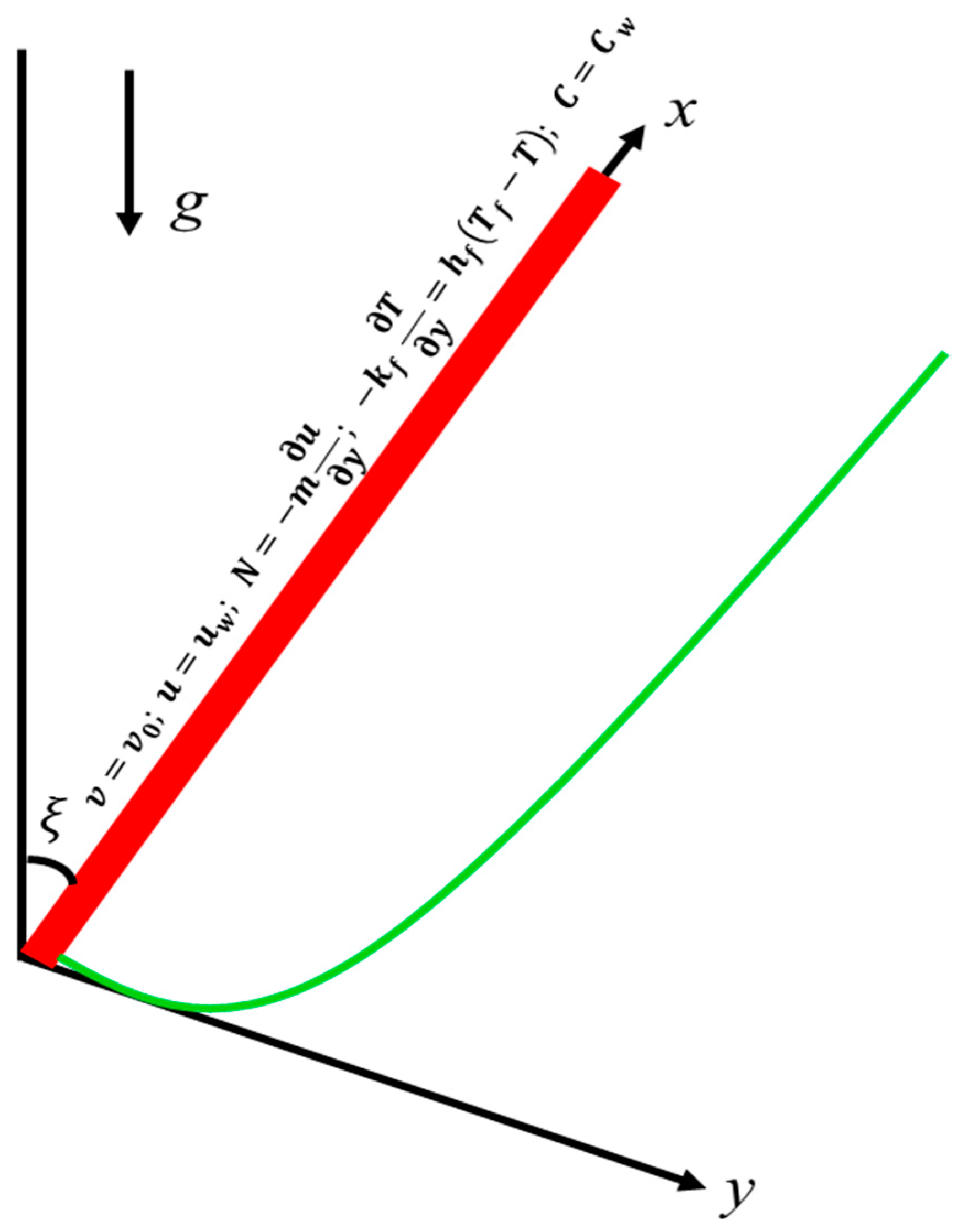
2. Problem Formulation

Two-dimensional steady flow of incompressible micropolar nanofluid on the linear inclined shrinking surface has been considered. Physical model and coordinate system of the problem is explained in Figure 1. Under the consideration of velocity and angular velocity field, temperature and nanoparticles volume fraction of the boundary layer equations for the flow of micropolar nanofluid can be written in the Buongiorno model [5] as below
  .   V = 0
ρ f d V d t = P + ( μ f + κ ) 2 V + κ ( × N ) + ρ f [ β T ( T T ) + β C ( C C ) ] g cos ξ
ρ f j d N d t = γ 2 N κ ( 2 N × V )
( ρ c ) p d T d t = k 2 T + ( ρ c ) f [ D B C   .   T + D T T ( T ) 2 ]
d C d t = D B 2 C + D T T 2 T
in which V [ u ( x , y ) , v ( x , y ) , 0 ] is the velocity vector, N is the microrotation vector, the spin gradient viscosity is γ , micro-rotation viscosity coefficient is κ , the gravitational acceleration is g , j is micro-inertia density, μ f , ρ f ,   p ,   D B ,   k , D T , ( ρ c ) f , ( ρ c ) p , and ξ stand for dynamic viscosity of base fluid, the densities of base fluid, pressure, the coefficient of Brownian motion, the thermal conductivity of base fluid, the thermophoretic diffusion coefficient, and the effective heat capacity of the base fluid, the effective heat capacity of the nanoparticle material, angle respectively. Further, T and C are the respective temperature and concentration, β T and β C are the respective coefficient of thermal and nanoparticle volumetric expansion.
According to scale analysis, we have the following boundary layer equations:
u x + v y = 0
u   u x   +   v   u y = ( ϑ f + κ ρ ) 2 u y 2 + κ ρ f N y + [ β T ( T T ) + β C ( C C ) ] g cos ξ
u N x + v N y = 1 ρ j [ γ 2 N y 2 κ ( 2 N + u y ) ]
u   T x   +   v   T y   = α f   2 T y 2   +   τ w   [ D B   C y   T y   +   D T T   ( T y ) 2 ]
u   C x   +   v   C y = D B   2 C y 2   +   D T T   2 T y 2
subject to boundary condition
v = v 0 ;   u = u w ;   N = m u y ;   k f   T y = h f ( T f T ) ;   C = C   w   a t   y = 0 u 0 ;   N 0 ;   T T ;   C C   a s   y
where u w = c x is the velocity of sheet and c is the constant, α f is the thermal diffusivity, τ w is the ratio of effective heat capacity, v 0 is the suction/injection parameter, C and T are the ambient concentration and temperature respectively, such that T f > T and C w > C . Following similarity will be used to get similarity solution of Equations (7)–(10) with subject to boundary conditions Equation (11). Moreover, m is the constant, where m = 0 which means that microelements are unable to rotate, when = 0 .5 which implies that antisymmetric part of the stress tensor is vanishing and where m = 1 which indicates the model of the turbulent flow.
η = y a ϑ f , u = a x f ( η ) , v = a ϑ f f ( η ) , N = a ϑ f a x g ( η ) , θ ( η ) = ( T T ) ( T f   T ) , ( η ) = ( C C ) C w C ,
By applying above relations and Equation (12) in Equations (7)–(10), we have
( 1 + K ) f + f f f 2 + K g + ( λ T θ + λ C ) cos ξ = 0
( 1 + K 2 )   g + f g g f 2 K g K f = 0
1 P r θ + f θ + N b θ + N t ( θ ) 2 = 0
1 S c + f + 1 S c N t N b θ = 0
along boundary conditions
f ( 0 ) = S ,   f ( 0 ) = λ , g ( 0 ) = m f ( 0 ) ,   θ ( 0 ) = B i [ 1 θ ( 0 ) ] ,   ( 0 ) = 1 f ( η )     0 ,   g ( η ) 0 ,   θ ( η ) 0 ,   ( η ) 0   a s   η
Here prime denotes the differentiation with respect to η , K = κ μ is the micropolar parameter, λ T = G r x T ( R e x ) 2 is the Buoyancy constraint where G r x T = g β T ( T T ) x 3 ϑ f ϑ f , λ C = G r x C ( R e x ) 2 is the buoyancy force due to concentration difference where G r x C = g β C ( T T ) x 3 ϑ f ϑ f , P r = ϑ f α f is the Prandtl number, N b = τ w D B ( C w C )   ϑ f , N t = τ w D T ( T f T )   ϑ f T are the Brownian motion and thermophoresis parameters. Moreover, S c = ϑ f D B is the Schmidt number, S = v 0 a ϑ f is the Suction/Blowing parameter, λ = c a is the stretching and shrinking parameter, and Biot number or convective parameter is i = h f k f ϑ f a .
The physically quantity of interest are Skin friction coefficient, local Nusselt number and local Sherwood number, which can be expressed as
C f = [ ( μ + κ ) u y + κ N ] y = 0 ρ u w 2 ,   N u = x [ k T y ] y = 0 ( T f   T ) ,   S h = x ( C y ) y = 0 C w C
Using Equation (12) in Equation (18), we have
C f ( R e x ) 1 2 = ( 1 + ( 1 m ) K ) f ( 0 ) ,   N u ( R e x ) 1 2 = θ ( 0 ) ,   S h ( R e x ) 1 2 = ( 0 )
where R e x = a x 2 / ϑ f is local Reynolds number.

3. Stability Analysis

The analysis of the stability of the solutions is a significant analysis to check the consistency of the multiple similarities as well as local similarity solutions. It is worth mentioning that a boundary layer problem might have one, zero, or multiple solutions. For instance, if there exist non-unique solutions in any boundary layer problem but the investigators succeed in obtaining one solution only, that solution may be the second solution (not real/unstable). It may prompt the distortion of the heat transfer attributes and flow. For dual solutions, the double set of initial suppositions (one (second) set for first (second) solution) are required to get two disparate profiles (solutions) of the velocity, temperature and concentration in the numerical method subject to condition that both the first and second profiles must asymptotically fulfill the boundary conditions. The following researchers have considered this analysis in their studies [46,47,48,49,50].
According to Merkin [51] and Dero et al. [52], the first stage in the stability analysis is to change the system of governing equations into a system of an unsteady problem by introducing τ = a t where t is the time since the disturbance may decay or grow with time. Thus, we have now following system of equations
u t + u   u x   +   v   u y = ( ϑ f + κ ρ ) 2 u y 2 + κ ρ f N y + [ β T ( T T ) + β C ( C C ) ] g cos ξ
N t + u N x + v N y = 1 ρ j [ γ 2 N y 2 κ ( 2 N + u y ) ]
T t + u   T x   +   v   T y   = α f   2 T y 2   +   τ w   [ D B   C y   T y   +   D T T   ( T y ) 2 ]
C t + u   C x   +   v   C y = D B   2 C y 2   +   D T T   2 T y 2
The new similarity transformation with τ = a t can be expressed as
η = y a ϑ f , τ = a t ,   u = a x f ( η ,   τ ) η , v = a ϑ f f ( η ,   τ ) , N = a ϑ f a x g ( η ,   τ ) , θ ( η , ,   τ ) = ( T T ) ( T w   T ) ,   ( η ,   τ ) = ( C C ) C w C ,  
Using Equation (24) into Equations (20)–(23), we get
( 1 + K ) 3 f η 3 + f 2 f η 2 ( f η ) 2 + K g η + ( λ T θ + λ C ) cos ξ 2 f τ η = 0
( 1 + K 2 )   2 g η 2 + f g η g f η Kg K 2 f η 2 g τ = 0
1 P r 2 θ η 2 + f θ η + N b η θ η + N t ( θ η ) 2 θ τ = 0
1 S c 2 η 2 + f η + 1 S c N t N b 2 θ η 2 τ = 0
with the following boundary conditions
f ( 0 , τ ) = S ;   f ( 0 ,   τ ) η = λ ;   g ( 0 , τ ) = m 2 f ( 0 ,   τ ) η 2 ;   θ ( 0 ,   τ ) η = B i [ 1 θ ( 0 ) ] ;   ( 0 , τ ) = 1 f ( η ,   τ ) η 0 ;   g ( η , τ ) 0 ;   θ ( η , τ ) 0 ; ( η , τ ) 0   a s   η
The following functions are used to obtain the behavior of the solution’s stability by perturbing with the disturbance [53].
{ f ( η , τ ) = f 0 ( η ) + e ε τ F ( η ) g ( η , τ ) = g 0 ( η ) + e ε τ G ( η ) θ ( η , τ ) = θ 0 ( η ) + e ε τ H ( η ) ( η , τ ) = 0 ( η ) + e ε τ S ( η )  
where F ( η ) , G ( η ) , H ( η ) , and S ( η ) are small relative to f 0 ( η ) , g 0 ( η ) , θ 0 ( η ) and 0 ( η ) , respectively. Further, f 0 ( η ) , g 0 ( η ) , θ 0 ( η ) and 0 ( η ) are the steady state solutions of the problem and ε is the unknown eigenvalue. Now, by substituting Equation (30) in Equations (25)–(28), we get following system of linearized eigenvalue problem
( 1 + K ) F 0 + f 0 F 0 + F 0 f 0 2 f 0 F 0 + K G 0 + + ( λ T H 0 + λ C S 0 ) cos ξ + ε F 0 = 0
( 1 + K 2 ) G 0 + f 0 G 0 + F 0 g 0 g 0 F 0 g 0 F 0 2 K G 0 K F 0 + ε G 0 = 0
1 P r H 0 + f 0 H 0 + F 0 θ 0 + N b 0 H 0 + N b S 0 θ 0 + 2 N t θ 0 H 0 + ε H 0 = 0
S 0 + S c ( f 0 0 + F 0 S 0 ) + N t N b H 0 + S c . ε S 0 = 0
with the boundary conditions
F 0 ( 0 ) = 0 ,   F 0 ( 0 ) = 0 ,   G 0 ( 0 ) = m F 0 ( 0 ) ,   H 0 = B i H 0 ( 0 ) ,   S 0 ( 0 ) = 0 F 0 ( η ) 0 ,   G 0 ( η ) 0 ,   H 0 ( η ) 0 ,   S 0 ( η ) 0   a s   η .  
According to Haris et al. [54], one boundary condition should be relaxed in the BVP4C solver to obtain the values of the smallest eigenvalue ε 1 . Here, F 0 ( η ) 0   a s   η is relaxed to F 0 ( 0 ) = 1 .

4. Numerical Method

It is very difficult to find the exact solutions for ODEs system when it contains non-linearity. In this case, researchers opted for numerical approach. Since we are dealing with highly non-linear system of ODEs Equations (13)–(16) subject to boundary conditions Equation (17), shooting method is adopted to solve the system. However, this system needs to be reduced to the equivalent system of first order ODEs as follows
p = f , q = p ; q = 1 ( 1 + K ) { p 2 f q K y 1 ( λ T θ + λ C ϕ ) cos ξ }  
y 1 = g ;   y 1 = 2 ( 2 + K ) { g p f y 1 + 2 K g + K q }  
r = θ ;   r = P r { f r N b s . r N t r 2 }  
s = ϕ ;   s = S c f s N t N b   r
subject to initial conditions
f ( 0 ) = S ; p ( 0 ) = λ ; q ( 0 ) = α 1 ; g ( 0 ) = m α 1 , y 1 ( 0 ) = α 2 ; θ ( 0 ) = 1 + α 3 Bi ; r ( 0 ) = α 3 ;   ϕ ( 0 ) = 1 ; s ( 0 ) = α 4
In order to solve Equations (36)–(39) subject to initial conditions Equation (40), the initial values α 1 , α 2 , α 3 and α 4 are required. These values are approximated by using the shooting method. Then, the resultant system of first order ODEs is solved by employing Runge–Kutta of 4th order. By assuming η = 10 , the calculated values of f ( η ) = 0 ; g ( η ) = 0 ;   θ ( η ) = 0 ; and   ( η ) = 0 are compared with given boundary condition f ( 10 ) = 0 ; g ( 10 ) = 0 ;   θ ( 10 ) = 0 ; and   ( 10 ) = 0 and the estimated values of α 1 , α 2 , α 3 and α 4 , are adjusted to obtain a better approximate solution.

5. Results and Discussion

In this section, the results of the considered problems are discussed. In this analysis, we have taken the Prandtl number for the water is Pr = 6.2 in order to check the effect of micropolar parameters over the inclined plane. The comparison and the authenticity of our numerical solution for the skin friction f ( 0 ) with the results of Bhattacharyya et al. [55] is portrayed in Figure 2 in which the latter solution is highlighted with the solid lines while the new solution is shown with the dashed lines. Further, our results are compared numerically for some selected values of N b and N t and found in a good agreement with Khan and Pop [56] as highlighted in Table 1. Table 2 displays the values of the smallest eigenvalue with fixed parameters λ T = 0.2 ,   λ C = 0.2 ,   ξ = 45 o ,   m = 0.5 ,   P r = 6.2 ,   N b = 0.3 ,   N t = 0.5 ,   S c = 1 ,   λ = 1   and   B i = 5 . It is noticed that the positive (negative) values of smallest eigenvalues ε 1 indicates that the first (second) solution is stable (unstable). The solution in this paper is obtained for both branches which we refer as dual solutions. Throughout the paper, the first solution is represented by the solid blue lines, while the second solution is represented by the dashed red lines. The critical points in all the figures is marked by the small green dot where both the solution behavior is changed at this position. These multiple solutions were found for different parameters and their results are plotted in distinct graphs.
Figure 3 was drawn for the skin friction coefficient along x-axis f ( 0 ) against the parameter S or various values of non-Newtonian parameter K . The critical points of K are S c 1 ,   S c 2 , and S c 3 where dual solutions exist. Moreover, after these points, there is no solution range. Absolute viscosity reduces for the higher values of the micropolar parameter due to this reduction, the first solution decreases. On the other hand, the dual trend is noticed in the second solution. Figure 4 shows the behavior of f ( 0 ) against λ for various values of angle ξ . The coefficient of skin friction is higher at the inclined plane in the first solution. Moreover, the dual solutions can be found in the shrinking case only. It is also noticed that λ has an inverse relation with the profile of f ( 0 ) . The impacts of the material parameter K on the g ( 0 ) for S are demonstrated in Figure 5. It is noticed that the couple’s stress coefficient is higher in the first solution for the higher values of the suction as resistance is created in the fluid flow. On the other hand, dual behavior is noticed in the second solution. Figure 6 is plotted to show the effect of λ on the g ( 0 ) for the various values of ξ . The behavior is revealed in Figure 4. Figure 7 depicts a decreasing behavior in both branches of the solution as the non-Newtonian parameter K is increased. It can be explained as a material parameter enhances the heat transfer rate due to the reduction in the absolute viscosity. As a result, the thickness of the thermal boundary layer becomes thinner. The impact of angle ξ on the θ ( 0 ) against the parameter λ is highlighted in Figure 8. The heat transfer rate reduces in both solutions when λ increases.
Figure 9 displays the influences of K on the rate of mass transfer ϕ ( 0 ) against S . It elucidates that both solutions are decelerating for the larger values of K . In general, it can be noticed that the concentration boundary layer is moving down when K is increased. The effects of the angle parameter ξ on the rate of mass transfer against the parameter λ is captured in Figure 10. The similar behavior of solutions is observed in Figure 10 as is noticed in Figure 9.
Figure 11 and Figure 12 show the behavior of the profiles for the f ( η ) and g ( η ) for the various values of the material parameter K , respectively. Figure 11 demonstrated that the momentum boundary layer is declined in the first solution and inclined in the second solution as K is increased for some fixed angle value ξ as highlighted in the above figure, while the impact of the same corresponding parameter on the g ( η ) is plotted in Figure 12 where the identical behavior is seen in the upper branch solution and the total reverse behavior is observed in the second branch solution. Figure 13, Figure 14 and Figure 15 are plotted in order to expose the behavior of temperature profile θ ( η ) for various values of N t thermophoresis parameter, B i the Biot number and the Brownian motion parameter N b , respectively. More exactly, it is scrutinized from Figure 13, Figure 14 and Figure 15 that when we are augmenting the values of N t , B i and N b , the temperature profile is boosted up in all the figures in both solutions, respectively.
Figure 16, Figure 17 and Figure 18 are designed in order to interpret the behavior of concentration profile ϕ ( η ) for various values of N t thermophoresis parameter, B i the Biot number and the Brownian motion parameter N b , respectively. Thus, it is investigated further, from Figure 16 and Figure 17 that when we augment the values of N t and B i the concentration boundary layer is larger in both branches of solutions, respectively, whilst the total reverse behavior is observed in Figure 18 for the augmentation of the Brownian motion parameter N b .

6. Conclusions

The two-dimensional steady flow of incompressible micropolar nanofluid on the linear inclined shrinking/stretching surface has been considered in the presence of convective condition. The self-similar equations are solved numerically. The microrotation and the angle ξ effect on the flow implements when the material parameter vagaries. It is observed that due to the augmentation in the micropolar parameter the steady flow needs more amount of mass suction and the stretching and shrinking parameter. More exactly, in all the phenomenon the dual similarity solutions for velocity, temperature and concentration exist. The skin friction coefficient, the heat transfer coefficient, the g ( 0 ) and the mass transfer rate decelerate in both solutions (first and second solution) against the mass suction parameter for the augmentation of the material parameter K , respectively. On the other hand, the impact of the angle parameter ξ against the parameter λ on the skin friction, mass transfer rate and g ( 0 ) shows an increasing behavior in both solutions whilst the reverse flow is observed for the heat transfer rate.

Author Contributions

Conceptualization, L.A.L. and Z.O.; Funding acquisition, D.B.; Investigation, U.K. and I.K.; Methodology, L.A.L., U.K. and I.K.; Project administration, I.K.; Software, L.A.L., I.K., Z.O., U.K. and K.S.N.; Supervision, I.K.; Review and Revision: D.B. and K.S.N.; Formal Analysis: D.B. and K.S.N. All authors have read and agreed to the published version of the manuscript.

Funding

This research received no external funding.

Acknowledgments

The authors are thankful to the Universiti Utara Malaysia (UUM) for supporting this work.

Conflicts of Interest

The authors declare no conflict of interest.

References

  1. Eringen, A.C. Simple micropolar fluids. Int. J. Eng. Sci. 1964, 2, 205–207. [Google Scholar] [CrossRef]
  2. Koriko, O.K.; Animasaun, I.L.; Omowaye, A.J.; Oreyeni, T. The combined influence of nonlinear thermal radiation and thermal stratification on the dynamics of micropolar fluid along a vertical surface. Multidiscip. Model. Mater. Struct. 2019, 15, 133–155. [Google Scholar] [CrossRef]
  3. Shah, Z.; Kumam, P.; Dawar, A.; Alzahrani, E.O.; Thounthong, P. Study of the Couple Stress Convective Micropolar Fluid Flow in a Hall MHD Generator System. Front. Phys. 2019, 7, 171. [Google Scholar] [CrossRef]
  4. Lukaszewicz, G. Micropolar Fluids: Theory and Applications; Brikhauser: Basel, Switzerland, 1999. [Google Scholar]
  5. Buongiorno, J. Convective transport in nanofluids. J. Heat Transf. 2006, 128, 240–250. [Google Scholar] [CrossRef]
  6. Hsiao, K.L. Micropolar nanofluid flow with MHD and viscous dissipation effects towards a stretching sheet with multimedia feature. Int. J. Heat Mass Transf. 2017, 112, 983–990. [Google Scholar] [CrossRef]
  7. Hayat, T.; Khan, M.I.; Waqas, M.; Alsaedi, A.; Khan, M.I. Radiative flow of micropolar nanofluid accounting thermophoresis and Brownian moment. Int. J. Hydrogen Energy 2017, 42, 16821–16833. [Google Scholar] [CrossRef]
  8. Noor, N.F.M.; Haq, R.U.; Nadeem, S.; Hashim, I. Mixed convection stagnation flow of a micropolar nanofluid along a vertically stretching surface with slip effects. Meccanica 2015, 50, 2007–2022. [Google Scholar] [CrossRef]
  9. Haq, R.U.; Nadeem, S.; Akbar, N.S.; Khan, Z.H. Buoyancy and radiation effect on stagnation point flow of micropolar nanofluid along a vertically convective stretching surface. IEEE Trans. Nanotechnol. 2014, 14, 42–50. [Google Scholar]
  10. Patel, H.R.; Mittal, A.S.; Darji, R.R. MHD flow of micropolar nanofluid over a stretching/shrinking sheet considering radiation. Int. Commun. Heat Mass Transf. 2019, 108, 104322. [Google Scholar] [CrossRef]
  11. Rafique, K.; Anwar, M.I.; Misiran, M. Numerical Study on Micropolar Nanofluid Flow over an Inclined Surface by Means of Keller-Box. Asian J. Probab. Stat. 2019, 1–21. [Google Scholar] [CrossRef]
  12. Rafique, K.; Anwar, M.I.; Misiran, M.; Khan, I.; Seikh, A.H.; Sherif, E.S.M.; Nisar, K.S. Numerical Analysis with Keller-Box Scheme for Stagnation Point Effect on Flow of Micropolar Nanofluid over an Inclined Surface. Symmetry 2019, 11, 1379. [Google Scholar] [CrossRef] [Green Version]
  13. Sithole, H.; Mondal, H.; Magagula, V.M.; Sibanda, P.; Motsa, S. Bivariate Spectral Local Linearisation Method (BSLLM) for unsteady MHD Micropolar-nanofluids with Homogeneous–Heterogeneous chemical reactions over a stretching surface. Int. J. Appl. Comput. Math. 2019, 5, 12. [Google Scholar] [CrossRef]
  14. Nadeem, S.; Abbas, N.; Elmasry, Y.; Malik, M.Y. Numerical analysis of water based CNTs flow of micropolar fluid through rotating frame. Comput. Methods Progr. Biomed. 2020, 186, 105194. [Google Scholar] [CrossRef]
  15. Ibrahim, W.; Gadisa, G. Finite element analysis of couple stress micropolar nanofluid flow by non-Fourier’s law heat flux model past stretching surface. Heat Transf. Asian Res. 2019. [Google Scholar] [CrossRef]
  16. Abbas, Z.; Mushtaq, T.; Shehzad, S.A.; Rauf, A.; Kumar, R. Slip flow of hydromagnetic micropolar nanofluid between two disks with characterization of porous medium. J. Braz. Soc. Mech. Sci. Eng. 2019, 41, 465. [Google Scholar] [CrossRef]
  17. Alzahrani, E.O.; Shah, Z.; Alghamdi, W.; Ullah, M.Z. Darcy–Forchheimer Radiative Flow of Micropoler CNT Nanofluid in Rotating Frame with Convective Heat Generation/Consumption. Processes 2019, 7, 666. [Google Scholar] [CrossRef] [Green Version]
  18. Abidi, A.; Raizah, Z.; Madiouli, J. Magnetic Field Effect on the Double Diffusive Natural Convection in Three-Dimensional Cavity Filled with Micropolar Nanofluid. Appl. Sci. 2018, 8, 2342. [Google Scholar] [CrossRef] [Green Version]
  19. Raslan, K.; Mohamadain, S.; Abdel-wahed, M.; Abedel-aal, E. MHD Steady/Unsteady Porous Boundary Layer of Cu–Water Nanofluid with Micropolar Effect over a Permeable Surface. Appl. Sci. 2018, 8, 736. [Google Scholar] [CrossRef] [Green Version]
  20. Anwar, M.I.; Shafie, S.; Hayat, T.; Shehzad, S.A.; Salleh, M.Z. Numerical study for MHD stagnation-point flow of a micropolar nanofluid towards a stretching sheet. J. Braz. Soc. Mech. Sci. Eng. 2017, 39, 89–100. [Google Scholar] [CrossRef] [Green Version]
  21. Lund, L.A.; Omar, Z.; Khan, I. Mathematical analysis of magnetohydrodynamic (MHD) flow of micropolar nanofluid under buoyancy effects past a vertical shrinking surface: Dual solutions. Heliyon 2019, 5, e02432. [Google Scholar] [CrossRef] [Green Version]
  22. Dero, S.; Rohni, A.M.; Saaban, A. MHD micropolar nanofluid flow over an exponentially stretching/shrinking surface: Triple solutions. J. Adv. Res. Fluid Mech. Therm. Sci. 2019, 56, 165–174. [Google Scholar]
  23. Magodora, M.; Mondal, H.; Sibanda, P. Dual solutions of a micropolar nanofluid flow with radiative heat mass transfer over stretching/shrinking sheet using spectral quasilinearization method. Multidiscip. Model. Mater. Struct. 2019. [Google Scholar] [CrossRef]
  24. Ali Lund, L.; Ching, D.L.C.; Omar, Z.; Khan, I.; Nisar, K.S. Triple local similarity solutions of Darcy-Forchheimer Magnetohydrodynamic (MHD) flow of micropolar nanofluid over an exponential shrinking surface: Stability analysis. Coatings 2019, 9, 527. [Google Scholar] [CrossRef] [Green Version]
  25. Turkyilmazoglu, M. Flow of a micropolar fluid due to a porous stretching sheet and heat transfer. Int. J. Non-Linear Mech. 2016, 83, 59–64. [Google Scholar] [CrossRef]
  26. Turkyilmazoglu, M. Mixed convection flow of magnetohydrodynamic micropolar fluid due to a porous heated/cooled deformable plate: Exact solutions. Int. J. Heat Mass Transf. 2017, 106, 127–134. [Google Scholar] [CrossRef]
  27. Lok, Y.Y.; Ishak, A.; Pop, I. Oblique stagnation slip flow of a micropolar fluid towards a stretching/shrinking surface: A stability analysis. Chin. J. Phys. 2018, 56, 3062–3072. [Google Scholar] [CrossRef]
  28. Lund, L.A.; Omar, Z.; Dero, S.; Khan, I. Linear stability analysis of MHD flow of micropolar fluid with thermal radiation and convective boundary condition: Exact solution. Heat Transf. Asian Res. 2019, 49. [Google Scholar] [CrossRef]
  29. Raza, J.; Rohni, A.M.; Omar, Z. Rheology of micropolar fluid in a channel with changing walls: Investigation of multiple solutions. J. Mol. Liq. 2016, 223, 890–902. [Google Scholar] [CrossRef]
  30. Mahmood, A.; Chen, B.; Ghaffari, A. Hydromagnetic Hiemenz flow of micropolar fluid over a nonlinearly stretching/shrinking sheet: Dual solutions by using Chebyshev Spectral Newton Iterative Scheme. J. Magn. Magn. Mater. 2016, 416, 329–334. [Google Scholar] [CrossRef]
  31. Sakiadis, B.C. Boundary-layer behavior on continuous solid surfaces: I. Boundary-layer equations for two-dimensional and axisymmetric flow. AIChE J. 1961, 7, 26–28. [Google Scholar]
  32. Raju, C.S.K.; Sandeep, N.; Babu, M.J.; Sugunamma, V. Dual solutions for three-dimensional MHD flow of a nanofluid over a nonlinearly permeable stretching sheet. Alex. Eng. J. 2016, 55, 151–162. [Google Scholar] [CrossRef] [Green Version]
  33. Li, X.; Khan, A.U.; Khan, M.R.; Nadeem, S.; Khan, S.U. Oblique Stagnation Point Flow of Nanofluids over Stretching/Shrinking Sheet with Cattaneo–Christov Heat Flux Model: Existence of Dual Solution. Symmetry 2019, 11, 1070. [Google Scholar] [CrossRef] [Green Version]
  34. Reddy, J.V.R.; Sugunamma, V.; Sandeep, N. Dual solutions for nanofluid flow past a curved surface with nonlinear radiation, Soret and Dufour effects. J. Phys. Conf. Ser. 2018, 1000, 012152. [Google Scholar] [CrossRef] [Green Version]
  35. Dero, S.; Uddin, M.J.; Rohni, A.M. Stefan blowing and slip effects on unsteady nanofluid transport past a shrinking sheet: Multiple solutions. Heat Transf. Asian Res. 2019, 48, 2047–2066. [Google Scholar] [CrossRef]
  36. Zaib, A.; Haq, R.U.; Sheikholeslami, M.; Khan, U. Numerical analysis of effective Prandtl model on mixed convection flow of γAl 2 O 3-H 2 O nanoliquids with micropolar liquid driven through wedge. Phys. Scr. 2019. [Google Scholar] [CrossRef]
  37. Khan, U.; Zaib, A.; Khan, I.; Nisar, K.S. Activation energy on MHD flow of titanium alloy (Ti6Al4V) nanoparticle along with a cross flow and streamwise direction with binary chemical reaction and non-linear radiation: Dual Solutions. J. Mater. Res. Technol. 2019. [Google Scholar] [CrossRef]
  38. Lund, L.A.; Omar, Z.; Khan, I.; Dero, S. Multiple solutions of Cu-C 6 H 9 NaO 7 and Ag-C 6 H 9 NaO 7 nanofluids flow over nonlinear shrinking surface. J. Cent. South Univ. 2019, 26, 1283–1293. [Google Scholar] [CrossRef]
  39. Jamaludin, A.; Nazar, R.; Pop, I. Mixed convection stagnation-point flow of a nanofluid past a permeable stretching/shrinking sheet in the presence of thermal radiation and heat source/sink. Energies 2019, 12, 788. [Google Scholar] [CrossRef] [Green Version]
  40. Mahanthesh, B.; Gireesha, B.J. Dual solutions for unsteady stagnation-point flow of Prandtl nanofluid past a stretching/shrinking plate. Defect Diffus. Forum 2018, 388, 124–134, Trans Tech Publications. [Google Scholar] [CrossRef]
  41. Ali Lund, L.; Omar, Z.; Khan, I.; Raza, J.; Bakouri, M.; Tlili, I. Stability Analysis of Darcy-Forchheimer Flow of Casson Type Nanofluid Over an Exponential Sheet: Investigation of Critical Points. Symmetry 2019, 11, 412. [Google Scholar] [CrossRef] [Green Version]
  42. Lund, L.A.; Omar, Z.; Khan, I.; Kadry, S.; Rho, S.; Mari, I.A.; Nisar, K.S. Effect of Viscous Dissipation in Heat Transfer of MHD Flow of Micropolar Fluid Partial Slip Conditions: Dual Solutions and Stability Analysis. Energies 2019, 12, 4617. [Google Scholar] [CrossRef] [Green Version]
  43. Junoh, M.M.; Md Ali, F.; Pop, I. Magnetohydrodynamics Stagnation-Point Flow of a Nanofluid Past a Stretching/Shrinking Sheet with Induced Magnetic Field: A Revised Model. Symmetry 2019, 11, 1078. [Google Scholar] [CrossRef] [Green Version]
  44. Revnic, C.; Ghalambaz, M.; Groşan, T.; Sheremet, M.; Pop, I. Impacts of Non-Uniform Border Temperature Variations on Time-Dependent Nanofluid Free Convection within a Trapezium: Buongiorno’s Nanofluid Model. Energies 2019, 12, 1461. [Google Scholar] [CrossRef] [Green Version]
  45. Khashi’ie, N.S.; Md Arifin, N.; Nazar, R.; Hafidzuddin, E.H.; Wahi, N.; Pop, I. A Stability Analysis for Magnetohydrodynamics Stagnation Point Flow with Zero Nanoparticles Flux Condition and Anisotropic Slip. Energies 2019, 12, 1268. [Google Scholar] [CrossRef] [Green Version]
  46. Mahapatra, T.R.; Nandy, S.K.; Vajravelu, K.; Van Gorder, R.A. Stability analysis of the dual solutions for stagnation-point flow over a non-linearly stretching surface. Meccanica 2012, 47, 1623–1632. [Google Scholar] [CrossRef]
  47. Mahapatra, T.R.; Nandy, S.K. Stability of dual solutions in stagnation-point flow and heat transfer over a porous shrinking sheet with thermal radiation. Meccanica 2013, 48, 23–32. [Google Scholar] [CrossRef]
  48. Barletta, A.; Rees, D.A.S. Stability analysis of dual adiabatic flows in a horizontal porous layer. Int. J. Heat Mass Transf. 2009, 52, 2300–2310. [Google Scholar] [CrossRef]
  49. Alarifi, I.M.; Abokhalil, A.G.; Osman, M.; Lund, L.A.; Ayed, M.B.; Belmabrouk, H.; Tlili, I. MHD flow and heat transfer over vertical stretching sheet with heat sink or source effect. Symmetry 2019, 11, 297. [Google Scholar] [CrossRef] [Green Version]
  50. Lund, L.A.; Omar, Z.; Khan, I. Quadruple solutions of mixed convection flow of magnetohydrodynamic nanofluid over exponentially vertical shrinking and stretching surfaces: Stability analysis. Comput. Method. Program. Biomed. 2019, 182, 105044. [Google Scholar] [CrossRef]
  51. Merkin, J.H. On dual solutions occurring in mixed convection in a porous medium. J. Eng. Math. 1986, 20, 171–179. [Google Scholar] [CrossRef]
  52. Dero, S.; Rohni, A.M.; Saaban, A.; Khan, I.; Seikh, A.H.; Sherif, E.-S.M.; Nisar, K.S. Dual Solutions and Stability Analysis of Micropolar Nanofluid Flow with Slip Effect on Stretching/Shrinking Surfaces. Energies 2019, 12, 4529. [Google Scholar] [CrossRef] [Green Version]
  53. Weidman, P.D.; Kubitschek, D.G.; Davis, A.M. The effect of transpiration on self-similar boundary layer flow over moving surfaces. Int. J. Eng. Sci. 2006, 44, 730–737. [Google Scholar] [CrossRef]
  54. Harris, S.D.; Ingham, D.B.; Pop, I. Mixed convection boundary-layer flow near the stagnation point on a vertical surface in a porous medium: Brinkman model with slip. Transp. Porous Med. 2009, 77, 267–285. [Google Scholar] [CrossRef]
  55. Bhattacharyya, K.; Mukhopadhyay, S.; Layek, G.C.; Pop, I. Effects of thermal radiation on micropolar fluid flow and heat transfer over a porous shrinking sheet. Int. J. Heat Mass Transf. 2012, 55, 2945–2952. [Google Scholar] [CrossRef]
  56. Khan, W.A.; Pop, I. Boundary-layer flow of a nanofluid past a stretching sheet. Int. J. Heat Mass Transf. 2010, 53, 2477–2483. [Google Scholar] [CrossRef]
Figure 1. Physical model and coordinate system.
Symmetry 12 00074 g001
Figure 2. Comparison of f ( 0 ) with results of Bhattacharyya et al., when m = 0.5 ,   λ = 1 ,   ξ = 90 ° .
Symmetry 12 00074 g002
Figure 3. f ( 0 ) versus the suction S for varying material parameter K .
Symmetry 12 00074 g003
Figure 4. f ( 0 ) versus the stretching/shrinking parameter λ for varying angle ξ .
Symmetry 12 00074 g004
Figure 5. g ( 0 ) versus the suction S for varying material parameter K .
Symmetry 12 00074 g005
Figure 6. g ( 0 ) versus the stretching/shrinking parameter λ for varying angle ξ .
Symmetry 12 00074 g006
Figure 7. θ ( 0 ) versus the suction S for varying material parameter K .
Symmetry 12 00074 g007
Figure 8. θ ( 0 ) versus the stretching/shrinking parameter λ for varying angle ξ .
Symmetry 12 00074 g008
Figure 9. ( 0 ) versus the suction S for varying material parameter K .
Symmetry 12 00074 g009
Figure 10. ( 0 ) versus the stretching/shrinking parameter λ for varying angle ξ .
Symmetry 12 00074 g010
Figure 11. f ( η ) for various values of material parameter K .
Symmetry 12 00074 g011
Figure 12. g ( η ) for various values of material parameter K .
Symmetry 12 00074 g012
Figure 13. θ ( η ) for various values of thermophoresis parameter N t .
Symmetry 12 00074 g013
Figure 14. θ ( η ) for various values of Biot number B i .
Symmetry 12 00074 g014
Figure 15. θ ( η ) for various values of Brownian motion parameter N b .
Symmetry 12 00074 g015
Figure 16. ϕ ( η ) for various values of thermophoresis parameter N t .
Symmetry 12 00074 g016
Figure 17. ϕ ( η ) for various values of Biot number B i .
Symmetry 12 00074 g017
Figure 18. ϕ ( η ) for various values of Brownian motion parameter N b .
Symmetry 12 00074 g018
Table 1. Comparison of results for the reduced Nusselt and Sherwood numbers when S = 0 ,   λ = 1 ,   B i = ,   ξ = 90 ° ,   K = 0 ,   S c = 10 ,   P r = 10.
N b N t Khan andPop [56]PresentResults
θ ( 0 ) ( 0 ) θ ( 0 ) ( 0 )
0.10.10.95242.12940.95242.1294
0.30.52012.52860.520052.5285
0.50.32113.03510.32123.0351
0.20.20.36542.51520.36542.5152
0.30.27312.65550.27312.6555
0.50.16812.88830.16812.8883
Table 2. Smallest eigen values for different values of K and S .
K S ε 1
1st Solution2nd Solution
031.53376−1.51742
2.51.08913−1.20287
20.97563−0.8101
0.530.86261−0.96571
2.50.54185−0.67231
20.05935−0.03765
130.45512−0.52843

