Efficient Three-Step Class of Eighth-Order Multiple Root Solvers and Their Dynamics

Abstract

This article proposes a wide general class of optimal eighth-order techniques for approximating multiple zeros of scalar nonlinear equations. The new strategy adopts a weight function with an approach involving the function-to-function ratio. An extensive convergence analysis is performed for the eighth-order convergence of the algorithm. It is verified that some of the existing techniques are special cases of the new scheme. The algorithms are tested in several real-life problems to check their accuracy and applicability. The results of the dynamical study confirm that the new methods are more stable and accurate than the existing schemes.

1. Introduction

Solving nonlinear problems is very important in numerical analysis and finds many applications in physics, engineering, and other applied sciences [1,2]. These problems occur in a variety of areas such as initial and boundary values, heat and fluid flow, electrostatics, or even in global positioning systems (GPS) [3,4,5,6]. It is difficult to find analytical solutions for nonlinear problems, but numerical techniques may be used to obtain approximate solutions. Therefore, iterative schemes provide an attractive alternative to solve such problems. When we discuss iterative solvers for finding multiple roots of nonlinear equations of the form $f\left(x\right)=0$, where $f\left(x\right)$ is a real function defined in a domain $D\subseteq \mathbb{R}$, we recall the classical modified Newton’s method [1,2,7] (also known as Rall’s algorithm), given by:

$$x_{n+1}=x_n-m\frac{f\left(x_n\right)}{f^{\prime }\left(x_n\right)},n=0,1,2,3,\cdots ,$$

(1)

where m is the multiplicity of the required solution. Given the multiplicity $m\ge 1$, in advance, the algorithm converges quadratically for multiple roots. We find one-point iterative functions in the literature, but in the scope of the real world, they are not of practical interest because of their theoretical limitations regarding convergence order and the efficiency index. Moreover, most of the one-point techniques are computationally expensive and inefficient when they are tested on numerical examples. Therefore, multipoint iterative algorithms are better candidates to qualify as efficient solvers. The good thing about multipoint iterative schemes without memory for scalar nonlinear equations is that we can establish a conjecture about their convergence order. According to the Kung–Traub conjecture [1], any multipoint method without memory can reach its convergence order of at most $2^{n-1}$ for n functional evaluations. A number of researchers proposed various optimal fourth-order techniques (requiring three functional evaluations per iteration) [8,9,10,11,12,13] and non-optimal approaches [14,15] for approximating multiple zeros of nonlinear functions. Nonetheless, a limited number of multipoint point iterative algorithms having a sixth-order of convergence were formulated. Thukral [16] proposed the following sixth-order multipoint iteration scheme:

$$\begin{array}{cc}\hfill y_n& =x_n-m\frac{f\left(x_n\right)}{f^{\prime }\left(x_n\right)},\hfill \\ \hfill z_n& =x_n-m\frac{f\left(x_n\right)}{f^{\prime }\left(x_n\right)}\sum _{i=1}^3{\left(\frac{f\left(y_n\right)}{f\left(x_n\right)}\right)}^{\frac{i}{m}},\hfill \\ \hfill x_{n+1}& =z_n-m\frac{f\left(x_n\right)}{f^{\prime }\left(x_n\right)}{\left(\frac{f\left(z_n\right)}{f\left(x_n\right)}\right)}^{\frac{1}{m}}{\left[\sum _{i=1}^3{\left(\frac{f\left(y_n\right)}{f\left(x_n\right)}\right)}^{\frac{i}{m}}\right]}^2.\hfill \end{array}$$

(2)

Geum et al. [17] presented a non-optimal class of two-point sixth-order as follows:

$$\begin{array}{ccc}\hfill y_n& =& x_n-m\frac{f\left(x_n\right)}{f^{\prime }\left(x_n\right)},m>1,\hfill \\ \hfill x_{n+1}& =& y_n-Q(u_n,s_n)\frac{f\left(y_n\right)}{f^{\prime }\left(y_n\right)},\hfill \end{array}$$

(3)

where $u_n=\sqrt[m]{\frac{f\left(y_n\right)}{f\left(x_n\right)}}$, $s_n=\sqrt[m-1]{\frac{f^{\prime }\left(y_n\right)}{f^{\prime }\left(x_n\right)}}$ and $Q:\mathbb{C}\to \mathbb{C}$ is a holomorphic function in the neighborhood of origin $(0,0)$. However, the main drawback of this algorithm is that it is not valid for simple zeros (i.e., for $m=1$).

In 2016, Geum et al. [18] developed another non-optimal family of three-point sixth-order techniques for multiple zeros consisting of the steps:

$$\begin{array}{ccc}\hfill y_n& =& x_n-m\frac{f\left(x_n\right)}{f^{\prime }\left(x_n\right)},m\ge 1,\hfill \\ \hfill w_n& =& y_n-mG\left(u_n\right)\frac{f\left(x_n\right)}{f^{\prime }\left(x_n\right)},\hfill \\ \hfill x_{n+1}& =& w_n-mK(u_n,v_n)\frac{f\left(x_n\right)}{f^{\prime }\left(x_n\right)},\hfill \end{array}$$

(4)

where $u_n=\sqrt[m]{\frac{f\left(y_n\right)}{f\left(x_n\right)}}$ and $v_n=\sqrt[m]{\frac{f\left(w_n\right)}{f\left(x_n\right)}}$. The weight functions $G:\mathbb{C}\to \mathbb{C}$ and $K:{\mathbb{C}}^2\to \mathbb{C}$ are analytic in the neighborhood of zero and $(0,0)$, respectively. It can be seen that (3) and (4) require four function evaluations to achieve sixth-order convergence. Therefore, they are not optimal in the sense of the Kung and Traub conjecture [1]. It is needless to mention that several authors have tried to develop optimal eighth-order techniques for multiple zeros, but without success to the authors’ best knowledge. Motivated by this fact, Behl et al. [19] introduced an optimal eighth-order iterative family for multiple roots given by:

$$\begin{array}{cc}\hfill y_n& =x_n-m\frac{f\left(x_n\right)}{f^{\prime }\left(x_n\right)},\hfill \\ \hfill z_n& =y_n-u_{n}Q\left(h_n\right)\frac{f\left(x_n\right)}{f^{\prime }\left(x_n\right)},\hfill \\ \hfill x_{n+1}& =z_n-u_n{v}_{n}G(h_n,v_n)\frac{f\left(x_n\right)}{f^{\prime }\left(x_n\right)},\hfill \end{array}$$

(5)

where $Q:\mathbb{C}\to \mathbb{C}$ is analytic in the neighborhood of $\left(0\right)$ and $G:{\mathbb{C}}^2\to \mathbb{C}$ is holomorphic in the neighborhood of $(0,0)$, with $u_n={\left(\frac{f\left(y_n\right)}{f\left(x_n\right)}\right)}^{\frac{1}{m}}$, $h_n=\frac{u_n}{a_1+a_2{u}_n}$, and $v_n={\left(\frac{f\left(z_n\right)}{f\left(y_n\right)}\right)}^{\frac{1}{m}}$. Moreover, $a_1$ and $a_2$ and free disposable real parameters.

Zafar et al. [20] presented an optimal eighth-order family using the weight function approach as follows:

$$\begin{array}{cc}\hfill y_n& =x_n-m\frac{f\left(x_n\right)}{f^{\prime }\left(x_n\right)},\hfill \\ \hfill z_n& =y_n-m{u}_{n}H\left(u_n\right)\frac{f\left(x_n\right)}{f^{\prime }\left(x_n\right)},\hfill \\ \hfill x_{n+1}& =z_n-u_n{v}_n(A_2+A_3{u}_n)P\left(v_n\right)G\left(w_n\right)\frac{f\left(x_n\right)}{f^{\prime }\left(x_n\right)},\hfill \end{array}$$

(6)

where $A_2$ and $A_3$ are real parameters and the weight functions $H,P,G:\mathbb{C}\to \mathbb{C}$ are analytic in the neighborhood of zero, with $u_n={\left(\frac{f\left(y_n\right)}{f\left(x_n\right)}\right)}^{\frac{1}{m}}$, $v_n={\left(\frac{f\left(z_n\right)}{f\left(y_n\right)}\right)}^{\frac{1}{m}}$, and $w_n={\left(\frac{f\left(z_n\right)}{f\left(x_n\right)}\right)}^{\frac{1}{m}}$.

It is clear from the above review of the state-of-the-art that we have a very small number of optimal eighth-order techniques that can handle the case of multiple zeros. Moreover, these types of methods have not been discussed in depth to date. Therefore, the main motivation of the current research work is to present a new optimal class of iterative functions having eighth-order convergence, exploiting the weight function technique for computing multiple zeros. The new scheme requires only four function evaluations $\left(\mathrm{i}.\mathrm{e}.,f\left(x_n\right),f^{\prime }\left(x_n\right),f\left(y_n\right)\mathrm{and}f\left(z_n\right)\right)$ per iteration, which is in accordance with the classical Kung–Traub conjecture. It is also interesting to note that the optimal eighth-order family (5) proposed by Behl et al. [19] can be considered as a special case of (7) for some particular values of the free parameters. In fact, the Artidiello et al. [21] family can be obtained as a special case of (7) in the case of simple roots. Therefore, the new algorithm can be treated as a more general family for approximating multiple zeros of nonlinear functions.

The rest of the paper is organized as follows. Section 2 presents the new eighth-order scheme and its convergence analysis. Section 2.1 discuss some special cases based on the different choices of weight functions employed in the second and third substeps of (7). Section 3 is devoted to the numerical experiments and the analysis of the dynamical behavior, which illustrate the efficiency, accuracy, and stability of (7). Section 4 presents the conclusions.

2. Construction of the Family

In this section, we develop a new optimal eighth-order scheme for multiple roots with known multiplicity $m\ge 1$. Here, we establish the main theorem describing the convergence analysis of the proposed family with the three steps as follows:

$$\begin{array}{cc}\hfill y_n& =x_n-m\frac{f\left(x_n\right)}{f^{\prime }\left(x_n\right)},\hfill \\ \hfill z_n& =y_n-m{u}_n\frac{f\left(x_n\right)}{f^{\prime }\left(x_n\right)}H\left(t_n\right),\hfill \\ \hfill x_{n+1}& =z_n-u_n{v}_n\frac{f\left(x_n\right)}{f^{\prime }\left(x_n\right)}G(t_n,s_n),\hfill \end{array}$$

(7)

where the weight functions H and G are such that $H:\mathbb{C}\to \mathbb{C}$ is analytic in the neighborhood of origin and $G:{\mathbb{C}}^2\to \mathbb{C}$ is holomorphic in the neighborhoods of $(0,0)$, with $u_n={\left(\frac{f\left(y_n\right)}{f\left(x_n\right)}\right)}^{\frac{1}{m}}$, $t_n=\frac{u_n}{b_1+b_2{u}_n}$, $v_n={\left(\frac{f\left(z_n\right)}{f\left(y_n\right)}\right)}^{\frac{1}{m}}$, and $s_n=\frac{v_n}{b_3+b_4{v}_n},$$b_i\in \mathbb{R}$ (for $i=1,2,3,4$) being arbitrary parameters.

In the following Theorem 1, we demonstrate how to construct weight functions H and G so that the algorithm arrives at the eighth order without requiring any additional functional evaluations.

Theorem 1.

Assume that $f:\mathbb{C}\to \mathbb{C}$ is an analytic function in the region enclosing the multiple zero $x=\alpha$ with multiplicity $m\ge 1$. The iterative Equation (7) has eighth-order convergence when it satisfies the conditions:

$$\left\{\begin{array}{c}H\left(0\right)=1,H^{\prime }\left(0\right)=2b_1,G_{00}=m,G_{10}=2m{b}_1,G_{01}=m{b}_3,\hfill \\ G_{20}=m(H^{″}\left(0\right)+2b_1^2),G_{11}=4m{b}_1{b}_3,G_{30}=m(H^{\left(3\right)}\left(0\right)+6b_1{H}^{″}\left(0\right)-24b_1^3-12b_1^2{b}_2),\hfill \end{array}\right.$$

(8)

where $G_{ij}={\displaystyle \frac{{\partial }^{i+j}G}{\partial t^i\partial s^j}}{|}_{(t=0,s=0)}$, $i,j\in \{0,1,2,3,4\}$.

Proof. 

Let $x=\alpha$ be a multiple zero of $f\left(x\right)$. Using the Taylor series expansion of $f\left(x_n\right)$ and $f^{\prime }\left(x_n\right)$ in the neighborhood of $\alpha$, we obtain:

$$f\left(x_n\right)=\frac{f^{\left(m\right)}\left(\alpha \right)}{m!}{e}_n^m\left(1+c_1{e}_n+c_2{e}_n^2+c_3{e}_n^3+c_4{e}_n^4+c_5{e}_n^5+c_6{e}_n^6+c_7{e}_n^7+c_8{e}_n^8+O\left(e_n^9\right)\right)$$

(9)

and:

$$\begin{array}{cc}\hfill f^{\prime }\left(x_n\right)=& \frac{f^m\left(\alpha \right)}{m!}{e}_n^{m-1}(m+c_1(m+1)e_n+c_2(m+2)e_n^2+c_3(m+3)e_n^3+c_4(m+4)e_n^4+c_5(m+5)e_n^5\hfill \\ & +c_6(m+6)e_n^6+c_7(m+7)e_n^7+c_8(m+8)e_n^8+O\left(e_n^9\right)),\hfill \end{array}$$

(10)

respectively, where $e_n=x_n-\alpha$, $c_k={\displaystyle \frac{1}{k!}}{\displaystyle \frac{f^{\left(k\right)}\left(\alpha \right)}{f^{\prime }\left(\alpha \right)}}$, and $k=1,2,3,\dots$.

Using the above Equations (9) and (10) in the first substep of (7), we get:

$$\begin{array}{cc}\hfill y_n-\alpha & =\frac{c_1{e}_n^2}{m}+\frac{(-(1+m)c_1^2+2m{c}_2)e_n^3}{m^2}+\sum _{j=1}^5{\Gamma }_j{e}_n^{j+3}+O\left(e_n^9\right),\hfill \end{array}$$

(11)

where ${\Gamma }_j={\Gamma }_j(m,c_1,c_2,\cdots ,c_8)$ are given in terms of $m,c_1,c_2,c_3,\cdots ,c_8$ for $1\le j\le 5$. The explicit expressions for the first two terms ${\Gamma }_1$ and ${\Gamma }_2$ are given by ${\Gamma }_1=\frac{1}{m^3}\{3m^2{c}_3+{(m+1)}^2{c}_1^3-m(3m+4)c_2{c}_1\}$ and ${\Gamma }_2=\frac{1}{m^4}\{{(m+1)}^3{c}_1^4-2m(2m^2+5m+3)c_2{c}_1^2+2m^2(2m+3)c_3{c}_1+2m^2(c_2^2(m+2)-2c_{4}m)\}$.

Using the Taylor series expansion again, we obtain:

$$\begin{array}{cc}\hfill f\left(y_n\right)=& f^{\left(m\right)}\left(\alpha \right)e_n^{2m}[\frac{\left(\frac{c_1}{m}\right){}^m}{m!}+\frac{(2c_{2}m-c_1^2(m+1)){\left(\frac{c_1}{m}\right)}^m{e}_n}{c_{1}m!}+{\left(\frac{c_1}{m}\right)}^{1+m}\frac{1}{2m!c_1^3}\{(3+3m+3m^2+m^3)c_1^4\hfill \\ & -2m(2+3m+2m^2)c_1^2{c}_2+4(-1+m)m^2{c}_2^2+6m^2{c}_1{c}_3\}{e}_n^2+\sum _{j=1}^5{\overline{\Gamma }}_j{e}_n^{j+3}+O\left(e_n^9\right)]\hfill \end{array}$$

(12)

and:

$$\begin{array}{cc}\hfill u_n& =\frac{c_1{e}_n}{m}+\frac{(2c_{2}m-c_1^2(m+2))e_n^2}{m^2}+{\gamma }_1{e}_n^3+{\gamma }_2{e}_n^4+{\gamma }_3{e}_n^5+O\left(e_n^6\right),\hfill \end{array}$$

(13)

where:

$$\left\{\begin{array}{cc}\hfill {\gamma }_1& =\frac{1}{2m^3}\left[c_1^3(2m^2+7m+7)+6c_3{m}^2-2c_2{c}_{1}m(3m+7)\right],\hfill \\ \hfill {\gamma }_2& =-\frac{1}{6m^4}[c_1^4(6m^3+29m^2+51m+34)-6c_2{c}_1^{2}m(4m^2+16m+17)+12c_3{c}_1{m}^2(2m+5)+12m^2(c_2^2(m+3)\hfill \\ & -2c_{4}m\left)\right],\hfill \\ \hfill {\gamma }_3& =\frac{1}{24m^5}[-24m^3(c_2{c}_3(5m+17)-5c_{5}m)+12c_3{c}_1^2{m}^2(10m^2+43m+49)+12c_1{m}^2\{c_2^2(10m^2+47m+53)\hfill \\ & -2c_{4}m(5m+13)\}-4c_2{c}_1^{3}m(30m^3+163m^2+306m+209)+c_1^5(24m^4+146m^3+355m^2+418m+209)].\hfill \end{array}\right.$$

(14)

Now, using the above Equation (14), we get:

$$\begin{array}{cc}\hfill t_n& =\frac{c_1}{m{b}_1}{e}_n+\sum _{i=1}^4{\Theta }_j{e}_n^{j+1}+O\left(e_n^6\right),\hfill \end{array}$$

(15)

where ${\Theta }_j={\Theta }_j(b_1,b_2,m,c_1,c_2,\cdots ,c_8)$ are given in terms of $b_1,b_2,m,c_1,c_2,\cdots ,c_8$, and the two coefficients ${\Theta }_1$ and ${\Theta }_2$ are written explicitly as ${\Theta }_1=-\frac{b_2{c}_1^2+b_1((2+m)c_1^2-2m{c}_2)}{m^2{b}_1^2},{\Theta }_2=\frac{1}{2m^3{b}_1^3}[2b_2^2{c}_1^3+4b_1{b}_2{c}_1((2+m)c_1^2-2m{c}_2)+b_1^2\{(7+7m+2m^2)c_1^3-2m(7+3m)c_1{c}_2+6m^2{c}_3\}]$.

Since we have $t_n={\displaystyle \frac{u_n}{b_1+b_2{u}_n}}=\mathcal{O}\left(e_n\right)$, it suffices to expand weight function $H\left(t_n\right)$ in the neighborhood of origin by means of Taylor expansion up to the fifth-order term, yielding:

$$H\left(t_n\right)\approx H\left(0\right)+H^{\prime }\left(0\right)t_n+\frac{1}{2!}{H}^{″}\left(0\right)t_n^2+\frac{1}{3!}{H}^{\left(3\right)}\left(0\right)t_n^3+\frac{1}{4!}{H}^{\left(4\right)}\left(0\right)t_n^4+\frac{1}{5!}{H}^{\left(5\right)}\left(0\right)t_n^5,$$

(16)

where $H^{\left(k\right)}$ represents the $k^{\mathrm{th}}$ derivative. By inserting the Equations (9)–(16) in the second substep of (7), we have:

$$\begin{array}{cc}\hfill z_n-\alpha =& \frac{(m-H\left(0\right))c_1}{m^2}{e}_n^2+\frac{2m(m-H\left(0\right))b_1{c}_2-\left(H^{\prime }\left(0\right)+(m+m^2-3H\left(0\right)-mH\left(0\right))b_1\right)c_1^2}{m^3{b}_1}{e}_n^3\hfill \\ & +\sum _{s=1}^5{\Omega }_s{e}_n^{s+3}+O\left(e_n^9\right),\hfill \end{array}$$

(17)

where ${\Omega }_s={\Omega }_s(H\left(0\right),H^{\prime }\left(0\right),H^{″}\left(0\right),H^{\left(3\right)}\left(0\right),H^{\left(4\right)}\left(0\right),m,b_1,b_2,c_1,c_2,\cdots ,c_8)$, $s=1,2,3,4,5$.

From the error Equation (17), it is clear that to obtain at least fourth-order convergence, the coefficients of $e_n^2$ and $e_n^3$ must vanish simultaneously. This result is possible only for the following values of $H\left(0\right)$ and $H^{\prime }\left(0\right)$, namely:

$$H\left(0\right)=m,H^{\prime }\left(0\right)=2m{b}_1,$$

(18)

which can be calculated from the Equation (17).

Substituting the above values of $H\left(0\right)$ and $H^{\prime }\left(0\right)$ in (17), we obtain:

$$\begin{array}{cc}\hfill z_n-\alpha & =\frac{(m(9+m)b_1^2-H^{″}\left(0\right)+4m{b}_1{b}_2)c_1^3-2m^2{b}_1^2{c}_1{c}_2}{2m^4{b}_1^2}{e}_n^4+\sum _{r=1}^4{L}_r{e}_n^{s+4}+O\left(e_n^9\right),\hfill \end{array}$$

(19)

where $L_r=L_r(H^{″}\left(0\right),H^{\left(3\right)}\left(0\right),H^{\left(4\right)}\left(0\right),m,b_1,b_2,c_1,c_2,\cdots ,c_8)$, $r=1,2,3,4$.

Using the Taylor series expansion again, we can write:

$$\begin{array}{c}\hfill f\left(z_n\right)=f^{\left(m\right)}\left(\alpha \right)e_n^{4m}\left[\frac{2^{-m}}{m!}\left(\frac{(m(9+m)b_1^2-H^{\prime \prime }\left(0\right)+4m{b}_1{b}_2)c_1^3-2m^2{b}_1^2{c}_1{c}_2}{m^4{b}_1^2}\right){}^m+\sum _{s=1}^5{\overline{P}}_s{e}_n^s+O\left(e_n^6\right)\right],\end{array}$$

(20)

and:

$$\begin{array}{cc}\hfill v_n=& \frac{(m(9+m)b_1^2-H^{″}\left(0\right)+4m{b}_1{b}_2)c_1^2-2m^2{b}_1^2{c}_2}{2m^3{b}_1^2}{e}_n^2+{\Delta }_1{e}_n^3+{\Delta }_2{e}_n^4+{\Delta }_3{e}_n^5+O\left(e_n^6\right),\hfill \end{array}$$

(21)

where ${\Delta }_1=\frac{1}{3m^4{b}_1^3}[3H^{″}\left(0\right)b_2{c}_1^3-12m{b}_1^2{b}_2{c}_1((3+m)c_1^2-2m{c}_2)+3b_1\left(((3+m)H^{″}\left(0\right)-2m{b}_2^2)c_1^3-2m{H}^{″}\left(0\right)c_1{c}_2\right)-m{b}_1^3\{(49+27m+2m^2)c_1^3-6m(9+m)c_1{c}_2+6m^2{c}_3\}]$.

Now, using the above Equation (21), we obtain:

$$\begin{array}{cc}\hfill s_n=\frac{v_n}{b_3+b_4{v}_n}=& \frac{(-H^{″}\left(0\right)+(9+m)b_1^2+4b_1{b}_2)c_1^2-2m{b}_1^2{c}_2}{2m^3{b}_1^2{b}_3}{e}_n^2+{\sigma }_1{e}_n^3+{\sigma }_2{e}_n^4+{\sigma }_3{e}_n^5+O\left(e_n^6\right),\hfill \end{array}$$

(22)

where ${\sigma }_i={\sigma }_i(m,b_1,b_2,b_3,b_4,H^{″}\left(0\right),H^{\left(3\right)}\left(0\right),c_1,c_2,c_3,c_4,c_5)$ for $1\le i\le 3,$ with the explicit coefficient ${\sigma }_1$ written as:

$$\begin{array}{cc}\hfill {\sigma }_1& =\frac{1}{6m^3{b}_1^3{b}_3}\left[\left(H^{\left(3\right)}\left(0\right)+\left(98+54m+4m^2\right)b_1^3-6H^{″}\left(0\right)b_2+24(3+m)b_1^2{b}_2-6b_1\left((3+m)H^{″}\left(0\right)-2b_2^2\right)\right)c_1^3\right.\hfill \\ & \left.-12m{b}_1\left(-H^{″}\left(0\right)+(9+m)b_1^2+4b_1{b}_2\right)c_1{c}_2+12m^2{b}_1^3{c}_3\right)].\hfill \end{array}$$

From Equations (15) and (22), we conclude that $t_n$ and $s_n$ are of orders $e_n$ and $e_n^2$, respectively. We can expand the weight function $G(t,s)$ in the neighborhood of $(0,0)$ by Taylor series up to fourth-order terms:

$$\begin{array}{cc}\hfill G(t_n,s_n)& \approx G_{00}+G_{10}{t}_n+G_{01}{s}_n+\frac{1}{2!}\left(G_{20}{t}_n^2+2G_{11}{t}_n{s}_n+G_{02}{s}_n^2\right)+\frac{1}{3!}\left(G_{30}{t}_n^3+3G_{21}{t}_n^2{s}_n+3G_{12}{t}_n{s}_n^2+G_{03}{s}_n^3\right)\hfill \\ & +\frac{1}{4!}\left(G_{40}{t}_n^4+4G_{31}{t}_n^3{s}_n+6G_{22}{t}_n^2{s}_n^2+4G_{13}{t}_n{s}_n^3+G_{04}{s}_n^4\right),\hfill \end{array}$$

(23)

where $G_{ij}=\frac{{\partial }^{i+j}}{\partial t^i\partial s^j}G(t,s){|}_{(t=0,s=0)}$, $i,j\in \{0,1,2,3,4\}$.

Using the Equations (9)–(23) in (7), we have:

$$\begin{array}{cc}\hfill e_{n+1}& =\frac{(G_{00}-m)c_1((H^{″}\left(0\right)-(m+9)b_1^2-4b_1{b}_2)c_1^2+2m{b}_1^2{c}_2)}{2b_1^2{m}^4}{e}_n^4+\sum _{i=1}^4{R}_i{e}_n^{i+4}+O\left(e_n^9\right),\hfill \end{array}$$

(24)

where $R_i=R_i(m,b_1,b_2,b_3,b_4,H\left(0\right),H^{\prime }\left(0\right),H^{″}\left(0\right),H^{\left(3\right)}\left(0\right),c_1,c_2,\cdots ,c_8)$, $i=1,2,3,4$.

To obtain at least sixth-order convergence, we need to adopt $G_{00}=m$. Furthermore, substituting $G_{00}=m$ in $R_1=0$, one obtains:

$$G_{10}=2b_{1}m.$$

(25)

Inserting $G_{00}=m$ and $G_{10}=2b_{1}m$ in $R_2=0$, we obtain the following relations:

$$G_{01}-m{b}_3=0,G_{20}-m{H}^{″}\left(0\right)-2m{b}_1^2=0,$$

(26)

which further yield:

$$G_{01}=m{b}_3,G_{20}=m{H}^{″}\left(0\right)+2m{b}_1^2.$$

(27)

By substituting the values of $G_{00}$, $G_{10}$, $G_{01}$, and $G_{20}$ in $R_3=0$, we obtain the following two independent equations:

$$\begin{array}{c}{G}_{11}-4b_1{b}_{3}m=0,\hfill \\ 3G_{11}{H}^{″}\left(0\right)-(G_{30}-m{H}^{\left(3\right)}\left(0\right))b_3+12m(7+m)b_1^3{b}_3-6b_1\left(2G_{11}{b}_2+m{H}^{″}\left(0\right)b_3\right)-3b_1^2\left(G_{11}(9+m)-12m{b}_2{b}_3\right)=0,\hfill \end{array}$$

(28)

which further give:

$$G_{11}=4b_1{b}_{3}m,G_{30}=m(H^{\left(3\right)}\left(0\right)+6b_1{H}^{″}\left(0\right)-24m{b}_1^3-12m{b}_1^2{b}_2).$$

(29)

Now, in order to obtain eighth-order convergence of the proposed scheme (7), the coefficients of $e_n^4$, $R_1,R_2,R_3$ defined in (24) must be equal to zero. Therefore, using the value of $G_{00}=m$ and substituting the values of $R_i^s$ (i = 1, 2, 3) from Relations (25)–(29) in (7), one gets the following error equation:

$$\begin{array}{cc}\hfill e_{n+1}& =\frac{1}{48m^8{b}_1^5{b}_3^2}\left[c_1(4b_2{c}_1^2+b_1((9+m)c_1^2-2m{c}_2)\right][-24G_{21}{b}_1{b}_2{b}_3{c}_1^4+(-G_{40}+m{H}^{\left(4\right)}\left(0\right))b_3^2{c}_1^4-24b_1^3{b}_2{c}_1^2\hfill \\ & \left(\left(G_{02}(9+m)-m(23+3m)b_3^2-2m(9+m)b_{3}b4\right)c_1^2+2m\left(-G_{02}+3m{b}_3^2+2m{b}_3{b}_4\right)c_2\right)-6b_1^2\left(4b_2^2\right(2G_{02}\hfill \\ & -3m{b}_3^2-4m{b}_3{b}_4)c_1^4+G_{21}{b}_3{c}_1^2\left((9+m)c_1^2-2m{c}_2\right))+.b_1^4\left(\right(-3G_{02}{(9+m)}^2+2m\left(431+102m+7m^2\right)b_3^2\hfill \\ & +6m{(9+m)}^2{b}_3{b}_4)c_1^4-12m\left(-G_{02}(9+m)+2m(17+2m)b_3^2+2m(9+m)b_3{b}_4\right)c_1^2{c}_2+12m^2(-G_{02}\hfill \\ & +2m{b}_3^2+2m{b}_3{b}_4)c_2^2+24m^3{b}_3^2{c}_1{c}_3)]e_n^8+O\left(e_n^9\right).\hfill \end{array}$$

(30)

The consequence of the above error analysis is that (7) acquires eighth-order convergence using only four functional evaluations (viz. $f\left(x_n\right),f^{\prime }\left(x_n\right),f\left(y_n\right)$ and $f\left(z_n\right)$) per full iteration. This completes the proof. □

2.1. Some Special Cases of the Proposed Class

In this section, we discuss some interesting special cases of the new class (7) by assigning different forms of weight functions $H\left(t_n\right)$ and $G(t_n,s_n)$ employed in the second and third steps, respectively.

• Let us consider the following optimal class of eighth-order methods for multiple roots, with the weight functions chosen directly from Theorem 1:

  $$\begin{array}{cc}\hfill y_n& =x_n-m\frac{f\left(x_n\right)}{f^{\prime }\left(x_n\right)},\hfill \\ \hfill z_n& =y_n-m{u}_n\frac{f\left(x_n\right)}{f^{\prime }\left(x_n\right)}\left[1+2t_n{b}_1+\frac{1}{2}{t}_n^2{H}^{″}\left(0\right)+\frac{1}{3!}{t}_n^3{H}^{\left(3\right)}\left(0\right)+\frac{1}{4!}{t}_n^4{H}^{\left(4\right)}\left(0\right)+\frac{1}{5!}{t}_n^5{H}^{\left(5\right)}\left(0\right)\right],\hfill \\ \hfill x_{n+1}& =z_n-u_n{v}_n\frac{f\left(x_n\right)}{f^{\prime }\left(x_n\right)}[m+2m{b}_1{t}_n+m{b}_3{s}_n+\frac{1}{2!}\left((H^{″}\left(0\right)m+2m{b}_1^2)t_n^2+8m{b}_1{b}_3{t}_n{s}_n+G_{02}{s}_n^2\right)\hfill \\ & +\frac{1}{3!}\left\{(H^{\left(3\right)}\left(0\right)+6H^{″}\left(0\right)b_1-24b_1^3-12b_1^2{b}_2)m{t}_n^3+3G_{21}{t}_n^2{s}_n+3G_{12}{t}_n{s}_n^2+G_{03}{s}_n^3\right\}\hfill \\ & +\frac{1}{4!}\left(G_{40}{t}_n^4+4G_{31}{t}_n^3{s}_n+6G_{22}{t}_n^2{s}_n^2+4G_{13}{t}_n{s}_n^3+G_{04}{s}_n^4\right)],\hfill \end{array}$$

  (31)

  where $b_i$ ($i=1,2,3,4$), $H^{″}\left(0\right),H^{\left(3\right)}\left(0\right),H^{\left(4\right)}\left(0\right),H^{\left(5\right)}\left(0\right)$, $G_{02},G_{12},G_{21},G_{03},G_{40},G_{31},G_{22},G_{13}$ and $G_{04}$ are free parameters.
  Subcases of the given scheme (31):

  (a)

  Let us consider $H^{″}\left(0\right)=H^{\left(3\right)}\left(0\right)=H^{\left(4\right)}\left(0\right)=H^{\left(5\right)}\left(0\right)=G_{02}=G_{12}=G_{21}=G_{03}=G_{31}=G_{22}=G_{13}=G_{04}=0$ in Equation (31). Then, we obtain:

  $$\begin{array}{cc}\hfill y_n& =x_n-m\frac{f\left(x_n\right)}{f^{\prime }\left(x_n\right)},\hfill \\ \hfill z_n& =y_n-m{u}_n\frac{f\left(x_n\right)}{f^{\prime }\left(x_n\right)}\left[1+2t_n{b}_1\right],\hfill \\ \hfill x_{n+1}& =z_n-u_n{v}_n\frac{f\left(x_n\right)}{f^{\prime }\left(x_n\right)}\left[m+m{s}_n{b}_3+2t_{n}m{b}_1(1+2s_n{b}_3)-4t_n^{3}m{b}_1^3+t_n^{2}m{b}_1^2(1-2t_n{b}_2)+\frac{G_{40}{t}_n^4}{24}\right].\hfill \end{array}$$

  (32)

• Considering $H^{″}\left(0\right)=H^{\left(3\right)}\left(0\right)=H^{\left(4\right)}\left(0\right)=H^{\left(5\right)}\left(0\right)=G_{12}=G_{03}=G_{31}=G_{22}=G_{13}=G_{04}=0$ and $G_{21}=2m$ in Equation (31), one gets:

  $$\begin{array}{cc}\hfill y_n& =x_n-m\frac{f\left(x_n\right)}{f^{\prime }\left(x_n\right)},\hfill \\ \hfill z_n& =y_n-m{u}_n\frac{f\left(x_n\right)}{f^{\prime }\left(x_n\right)}\left[1+2t_n{b}_1\right],\hfill \\ \hfill x_{n+1}& =z_n-u_n{v}_n\frac{f\left(x_n\right)}{f^{\prime }\left(x_n\right)}\left[m{s}_n{t}_n^2+\frac{G_{02}}{2}{s}_n^2+m\left(1-4b_1^3{t}_n^3+b_1^2\left(t_n^2-2b_2{t}_n^3\right)+b_3{s}_n+2b_1(t_n+2b_3{t}_n{s}_n)\right)\right].\hfill \end{array}$$

  (33)
• A combination of polynomial and rational functions produces another optimal eighth-order scheme as follows:

  $$\begin{array}{cc}\hfill y_n& =x_n-m\frac{f\left(x_n\right)}{f^{\prime }\left(x_n\right)},\hfill \\ \hfill z_n& =y_n-m{u}_n\frac{f\left(x_n\right)}{f^{\prime }\left(x_n\right)}\left[1+2t_n{b}_1\right],\hfill \\ \hfill x_{n+1}& =z_n-u_n{v}_n\frac{f\left(x_n\right)}{f^{\prime }\left(x_n\right)}\left[k_1{t}_n^2+k_2{s}_n+{\displaystyle \frac{k_3{t}_n^2+k_4{t}_n+k_5{s}_n+k_6}{k_7{t}_n+s_n+1}}\right],\hfill \end{array}$$

  (34)

  where:

  $$\left\{\begin{array}{c}{k}_1={\displaystyle \frac{m\left(-24b_1^3+6b_1^2(-2b_2+k_7)\right)}{6k_7}},\hfill \\ k_2={\displaystyle \frac{m\left(b_1(2+4b_3)+b_3{k}_7\right)}{k_7}},\hfill \\ k_3={\displaystyle \frac{m\left(24b_1^3+12b_1^2{b}_2+12b_1{k}_7^2\right)}{6k_7}},\hfill \\ k_4=m\left(2b_1+k_7\right),\hfill \\ k_5={\displaystyle \frac{m\left(-2b_1(1+2b_3)+k_7\right)}{k_7}},\hfill \\ k_6=m.\hfill \end{array}\right.$$

  (35)

Remark 1.

It is important to note that the weight functions $H\left(t_n\right)$ and $G(t_n,s_n)$ play a significant role in the construction of eighth-order techniques. Therefore, it is usual to display different choices of weight functions, provided they satisfy all the conditions of Theorem 1. Hence, we discussed above some special cases (32), (33), and (35) having simple body structures along with optimal eight-order convergence so that they can be easily implemented in numerical experiments.

Remark 2.

The family (5) proposed by Behl et al. [19] can be obtained as a special case of (7) by selecting suitable values of free parameters as, namely, $b_1=a_1$, $b_2=a_2$, $b_3=1$, and $b_4=0$.

3. Numerical Experiments

In this section, we analyze the computational aspects of the following cases: Equation (32) for $(b_1=1,b_2=-2,b_3=1,b_4=-2,G_{40}=0)$ ($MM1$), Family (33) for $(b_1=1,b_2=-2,b_3=1,b_4=-2,G_{02}=0)$ ($MM2$), and Equation (35) for $(b_1=1,b_2=-2,b_3=1,b_4=-2,k_7=-\frac{3}{10})$ ($MM3$). Additionally, we compare the results with those of other techniques.

In this regard, we considered several test functions coming from real-life problems and linear algebra that represent Examples 1–7 in the follow-up. We compared them with the optimal eighth-order scheme (5) given by Behl et al. [19] for $Q\left(h_n\right)=m(1+2h_n+3h_n^2)$ and $G(h_n,t_n)=m\left(\frac{1+2t_n+3h_n^2+h_n(2+6t_n+h_n)}{1+t_n}\right)$ and the approach (6) of Zafar et al. [20] taking $H\left(u_n\right)=6u_n^3-u_n^2+2u_n+1$, $P\left(v_n\right)=1+v_n$, and $G\left(w_n\right)=\frac{2w_n+1}{A_2{P}_0}$ for $(A_2=P_0=1)$ denoted by $\left(OM\right)$ and $\left(ZM\right)$, respectively. Furthermore, we compared them with the family of two-point sixth-order methods proposed by Geum et al. in [17], choosing out of them Case 2A, given by:

$$\begin{array}{cc}\hfill y_n& =x_n-m\frac{f\left(x_n\right)}{f^{\prime }\left(x_n\right)},m>1,\hfill \\ \hfill x_{n+1}& =y_n-\left[\frac{m+b_1{u}_n}{1+a_1{u}_n+a_2{s}_n+a_3{s}_n{u}_n}\right]\frac{f\left(y_n\right)}{f^{\prime }\left(y_n\right)},\hfill \end{array}$$

(36)

where $a_1=-\frac{2m(m-2)}{(m-1)}$, $b_1=\frac{2m}{(m-1)}$, $a_2=2(m-1)$, and $a_3=3$.

Finally, we compared them with the non-optimal family of sixth-order methods based on the weight function approach presented by Geum et al. [18]; out of them, we considered Case 5YD, which is defined as follows:

$$\begin{array}{cc}\hfill y_n& =x_n-m\frac{f\left(x_n\right)}{f^{\prime }\left(x_n\right)},m\ge 1,\hfill \\ \hfill w_n& =x_n-m\left[\frac{\left(u_n-2\right)\left(2u_n-1\right)}{\left(u_n-1\right)\left(5u_n-2\right)}\right]\frac{f\left(x_n\right)}{f^{\prime }\left(x_n\right)},\hfill \\ \hfill x_{n+1}& =x_n-m\left[\frac{\left(u_n-2\right)\left(2u_n-1\right)}{\left(5u_n-2\right)\left(u_n+v_n-1\right)}\right]\frac{f\left(x_n\right)}{f^{\prime }\left(x_n\right)}.\hfill \end{array}$$

(37)

We denote Equations (36) and (37) by $\left(GK1\right)$ and $\left(GK2\right)$, respectively.

The numerical results listed in

Table 1. Convergence behavior of seven different iterative methods on the test function $f_1\left(x\right)$.

Methods	n	${\mathit{x}}_{\mathit{n}}$	$\left|\mathit{f}\right({\mathit{x}}_{\mathit{n}}\left)\right|$	$|{\mathit{x}}_{\mathit{n}+1}-{\mathit{x}}_{\mathit{n}}|$	$\mathit{\rho }$	$\left|\frac{{\mathit{x}}_{\mathit{n}+1}-{\mathit{x}}_{\mathit{n}}}{{({\mathit{x}}_{\mathit{n}}-{\mathit{x}}_{\mathit{n}-1})}^8}\right|$	$\mathit{\eta }$
$GK1$	0	$1.8$	$2.0(-4)$	$4.9(-2)$
	1	$1.750895258580091535641280$	$2.5(-8)$	$9.0(-4)$		$6.385691220(+4)$	$3.536522620(+7)$
	2	$1.750000000014299761415271$	$6.1(-24)$	$1.4(-11)$		$2.777396484(+7)$
	3	$1.750000000000000000000000$	$2.7(-117)$	$3.0(-58)$	$5.9816$	$3.536522620(+7)$
$GK2$	0	$1.8$	$2.0(-4)$	$5.0(-2)$
	1	$1.750388172793891559741273$	$4.6(-9)$	$3.9(-4)$		$2.603237303(+4)$	$3.215020576(+6)$
	2	$1.750000000000010343224637$	$3.2(-30)$	$1.0(-14)$		$3.023468138(+6)$
	3	$1.750000000000000000000000$	$4.6(-157)$	$3.9(-78)$	$5.9959$	$3.215020576(+6)$
$OM$	0	$1.8$	$2.0(-4)$	$4.9(-2)$
	1	$1.750388172319823575363680$	$9.9(-9)$	$5.7(-4)$		$1.599594295(+7)$	$1.462834362(+11)$
	2	$1.750000000000001356336629$	$5.5(-32)$	$1.4(-15)$		$3.750857339(+11)$
	3	$1.750000000000000000000000$	$8.4(-218)$	$1.7(-108)$	$7.9903$	$1.462834362(+11)$
$ZM$	0	$1.8$	$2.0(-4)$	$5.0(-2)$
	1	$1.750388172319823575363680$	$4.6(-9)$	$3.9(-4)$		$1.057651892(+7)$	$1.178394347(+11)$
	2	$1.750000000000000051608567$	$8.0(-35)$	$5.2(-17)$		$1.001210273(+11)$
	3	$1.750000000000000000000000$	$1.1(-240)$	$5.9(-120)$	$7.9928$	$1.178394347(+11)$
$MM1$	0	$1.8$	$2.0(-4)$	$5.0(-2)$
	1	$1.750083046950291853331587$	$2.1(-10)$	$8.3(-5)$		$2.154463519(+6)$	$2.545224623(+9)$
	2	$1.750000000000000000000006$	$9.5(-49)$	$5.6(-24)$		$2.493663476(+9)$
	3	$1.750000000000000000000000$	$2.0(-355)$	$2.6(-177)$	$7.9993$	$2.545224623(+9)$
$MM2$	0	$1.8$	$2.0(-4)$	$5.0(-2)$
	1	$1.750071038018750802896248$	$1.5(-10)$	$7.1(-5)$		$1.639376116(+6)$	$1.741469479(+9)$
	2	$1.750000000000000000000001$	$3.7(-50)$	$1.1(-24)$		$1.712046103(+9)$
	3	$1.750000000000000000000000$	$4.9(-367)$	$4.0(-183)$	$7.9994$	$1.741469479(+9)$
$MM3$	0	$1.8$	$2.0(-4)$	$4.9(-2)$
	1	$1.750570071950781672220702$	$1.5(-8)$	$7.0(-4)$		$2.002134740(+7)$	$2.569337277(+10)$
	2	$1.750000000000001356336629$	$4.6(-32)$	$1.2(-15)$		$2.174278591(+10)$
	3	$1.750000000000000000000000$	$5.9(-220)$	$1.4(-109)$	$7.9904$	$2.569337277(+10)$

,

Table 2. Convergence behavior of seven different iterative methods on the test function $f_2\left(x\right)$.

Methods	n	${\mathit{x}}_{\mathit{n}}$	$\left|\mathit{f}\right({\mathit{x}}_{\mathit{n}}\left)\right|$	$|{\mathit{x}}_{\mathit{n}+1}-{\mathit{x}}_{\mathit{n}}|$	$\mathit{\rho }$	$\left|\frac{{\mathit{x}}_{\mathit{n}+1}-{\mathit{x}}_{\mathit{n}}}{{({\mathit{x}}_{\mathit{n}}-{\mathit{x}}_{\mathit{n}-1})}^8}\right|$	$\mathit{\eta }$
$GK1$	0	$0.76$	*	*
	1		*	*		*	*
	2		*	*		*
	3		*	*	*	*
$GK2$	0	$0.76$	$2.2(-1)$	$2.6(-3)$
	1	$0.7573962460753336221899798$	$1.4(-8)$	$1.8(-10)$		$5.725910242(+5)$	$5.257130496(+5)$
	2	$0.7573962462537538794596413$	$1.4(-51)$	$1.7(-53)$		$5.257130467(+5)$
	3	$0.7573962462537538794596413$	$1.0(-309)$	$1.3(-311)$	$6.0000$	$5.257130496(+5)$
$OM$	0	$0.76$	$2.2(-1)$	$2.6(-3)$
	1	$0.7573962463137703385994168$	$4.8(-9)$	$6.0(-11)$		$2.840999693(+10)$	$3.013467463(+10)$
	2	$0.7573962462537538794596413$	$4.0(-70)$	$5.1(-72)$		$3.013467461(+10)$
	3	$0.7573962462537538794596413$	$1.1(-558)$	$1.3(-560)$	$8.0000$	$3.013467463(+10)$
$ZM$	0	$0.76$	$2.2(-1)$	$2.6(-3)$
	1	$0.7573962463048948508621891$	$4.1(-9)$	$5.1(-11)$		$2.420860580(+10)$	$3.421344786(+10)$
	2	$0.7573962462537538794596413$	$1.3(-70)$	$1.6(-72)$		$3.421344762(+10)$
	3	$0.7573962462537538794596413$	$1.2(-562)$	$1.5(-564)$	$8.0000$	$3.421344786(+10)$
$MM1$	0	$0.76$	$2.2(-1)$	$2.6(-3)$
	1	$0.7573962462537574111428461$	$2.8(-13)$	$3.5(-15)$		$1.671792904(+6)$	$1.186467025(+6)$
	2	$0.7573962462537538794596413$	$2.3(-108)$	$2.9(-110)$		$1.186467025(+6)$
	3	$0.7573962462537538794596413$	$4.4(-869)$	$5.5(-871)$	$8.0000$	$1.186467025(+6)$
$MM2$	0	$0.76$	$2.2(-1)$	$2.6(-3)$
	1	$0.7573962462537553703375248$	$1.2(-13)$	$1.5(-15)$		$7.057368744(+5)$	$4.421886626(+5)$
	2	$0.7573962462537538794596413$	$8.6(-112)$	$1.1(-113)$		$4.421886626(+5)$
	3	$0.7573962462537538794596413$	$6.5(-897)$	$8.1(-899)$	$8.0000$	$4.421886626(+5)$
$MM3$	0	$0.76$	$2.2(-1)$	$2.6(-3)$
	1	$0.7573962462537526002632867$	$1.0(-13)$	$1.3(-15)$		$6.055331876(+5)$	$5.153221799(+5)$
	2	$0.7573962462537538794596413$	$2.9(-112)$	$3.7(-114)$		$5.153221799(+5)$
	3	$0.7573962462537538794596413$	$1.4(-900)$	$1.8(-902)$	$8.0000$	$5.153221799(+5)$

(* means: the corresponding method does not work.)

,

Table 3. Convergence behavior of seven different iterative methods on the test function $f_3\left(x\right)$.

Methods	n	${\mathit{x}}_{\mathit{n}}$	$\left|\mathit{f}\right({\mathit{x}}_{\mathit{n}}\left)\right|$	$|{\mathit{x}}_{\mathit{n}+1}-{\mathit{x}}_{\mathit{n}}|$	$\mathit{\rho }$	$\left|\frac{{\mathit{x}}_{\mathit{n}+1}-{\mathit{x}}_{\mathit{n}}}{{({\mathit{x}}_{\mathit{n}}-{\mathit{x}}_{\mathit{n}-1})}^8}\right|$	$\mathit{\eta }$
$GK1$	0	$-3.0$	$4.7(-2)$	$1.5(-1)$
	1	$-2.850032149435759899649078$	$2.2(-9)$	$3.2(-5)$		$2.826079363(+0)$	$4.198827967(-5)$
	2	$-2.850000000000000000000000$	$4.5(-63)$	$4.6(-32)$		$4.191188565(-5)$
	3	$-2.850000000000000000000000$	$3.6(-385)$	$4.1(-193)$	$6.0000$	$4.198827967(-5)$
$GK2$	0	$-3.0$	$4.7(-2)$	$1.5(-1)$
	1	$-2.845530536829933778640841$	$4.2(-5)$	$4.5(-3)$		$3.291554609(+2)$	$1.360955722(-3)$
	2	$-2.850002074441970615144759$	$9.0(-12)$	$2.1(-6)$		$2.595135041(+8)$
	3	$-2.850000000000000000000000$	$2.5(-74)$	$1.1(-37)$	$9.3846$	$1.360955722(-3)$
$OM$	0	$-3.0$	$4.7(-2)$	$1.6(-1)$
	1	$-2.844042602118935658056506$	$7.5(-5)$	$6.0(-3)$		$1.703635813(+4)$	$6.783289282(-4)$
	2	$-2.850005050121091781574571$	$5.4(-11)$	$5.1(-6)$		$3.161585672(+12)$
	3	$-2.850000000000000000000000$	$1.7(-91)$	$2.9(-46)$	$13.102$	$6.783289282(-4)$
$ZM$	0	$-3.0$	$4.7(-2)$	$1.6(-1)$
	1	$-2.840827596075196247341513$	$1.8(-4)$	$9.2(-3)$		$2.230697732(+4)$	$3.402776481(-4)$
	2	$-2.850019022777759525868734$	$7.6(-10)$	$1.9(-5)$		$3.734311208(+11)$
	3	$-2.850000000000000000000000$	$7.1(-83)$	$5.8(-42)$	$13.609$	$3.402776481(-4)$
$MM1$	0	$-3.0$	$4.7(-2)$	$1.5(-1)$
	1	$-2.847075767557386926817015$	$1.8(-5)$	$2.9(-3)$		$9.778827612(+3)$	$3.201998473(-4)$
	2	$-2.850000574904908612754099$	$6.9(-13)$	$5.7(-7)$		$1.073539173(+14)$
	3	$-2.850000000000000000000000$	$3.1(-107)$	$3.8(-54)$	$12.729$	$3.201998473(-4)$
$MM2$	0	$-3.0$	$4.7(-2)$	$1.5(-1)$
	1	$2.847075846659888868138671$	$1.8(-5)$	$2.9(-3)$		$9.778603498(+3)$	$3.209704581(-4)$
	2	$-2.850000574872938822686310$	$6.9(-13)$	$5.7(-7)$		$1.073711858(+14)$
	3	$-2.850000000000000000000000$	$3.1(-107)$	$3.8(-54)$	$12.728$	$3.209704581(-4)$
$MM3$	0	$-3.0$	$4.7(-2)$	$9.4(-2)$
	1	$-2.905607206926252789906690$	$6.5(-3)$	$5.5(-2)$		$8.756793722(+6)$	$6.122326772(-3)$
	2	$-2.850417788760620872669269$	$3.7(-7)$	$4.2(-4)$		$4.854116866(+6)$
	3	$-2.850000000000000000000000$	$6.8(-59)$	$5.7(-30)$	$12.176$	$6.122326772(-3)$

,

Table 4. Convergence behavior of seven different iterative methods on the test function $f_4\left(x\right)$.

Methods	n	${\mathit{x}}_{\mathit{n}}$	$\left|\mathit{f}\right({\mathit{x}}_{\mathit{n}}\left)\right|$	$|{\mathit{x}}_{\mathit{n}+1}-{\mathit{x}}_{\mathit{n}}|$	$\mathit{\rho }$	$\left|\frac{{\mathit{x}}_{\mathit{n}+1}-{\mathit{x}}_{\mathit{n}}}{{({\mathit{x}}_{\mathit{n}}-{\mathit{x}}_{\mathit{n}-1})}^8}\right|$	$\mathit{\eta }$
$GK1$	0	$2.1$	$9.8(-25)$	$1.0(-1)$
	1	$2.000002777374011867781357$	$1.1(-254)$	$2.8(-6)$		$2.777836885(+00)$	$5.504789671(+00)$
	2	$2.000000000000000000000000$	$9.6(-1607)$	$2.5(-33)$		$5.504677538(+00)$
	3	$2.000000000000000000000000$	$4.5(-9719)$	$1.4(-195)$	$6.0000$	$5.504789671(+00)$
$GK2$	0	$2.1$	$9.8(-25)$	$1.0(-1)$
	1	$2.000000200989638086020762$	$1.0(-311)$	$2.0(-7)$		$2.009920619(-1)$	$2.777777778(-1)$
	2	$2.000000000000000000000000$	$9.8(-2014)$	$1.8(-41)$		$2.777775861(-1)$
	3	$2.000000000000000000000000$	$7.3(-12226)$	$1.0(-245)$	$6.0000$	$2.777777778(-1)$
$OM$	0	$2.1$	$9.8(-25)$	$1.0(-1)$
	1	$2.000000785189010712446522$	$4.0(-282)$	$7.9(-7)$		$7.852383342(+1)$	$2.269259259(+2)$
	2	$2.000000000000000000000000$	$4.4(-2301)$	$3.3(-47)$		$2.269242109(+2)$
	3	$2.000000000000000000000000$	$8.3(-18453)$	$3.0(-370)$	$8.0000$	$2.269259259(+2)$
$ZM$	0	$2.1$	$9.8(-25)$	$1.0(-1)$
	1	$2.000000477890417235498042$	$6.6(-293)$	$4.8(-7)$		$4.779086880(+1)$	$2.084074074(+2)$
	2	$2.000000000000000000000000$	$3.4(-2389)$	$5.7(-49)$		$2.084057463(+2)$
	3	$2.000000000000000000000000$	$1.6(-19159)$	$2.2(-384)$	$8.0000$	$2.084074074(+2)$
$MM1$	0	$2.1$	$9.8(-25)$	$1.0(-1)$
	1	$2.000000007342778263970301$	$1.4(-383)$	$7.3(-9)$		$7.342782577(-1)$	$1.259259259(+00)$
	2	$2.000000000000000000000000$	$1.6(-3225)$	$1.1(-65)$		$1.259259209(+00)$
	3	$2.000000000000000000000000$	$4.6(-25961)$	$2.1(-520)$	$8.0000$	$1.259259259(+00)$
$MM2$	0	$2.1$	$9.8(-25)$	$1.0(-1)$
	1	$2.000000004907980605841013$	$2.5(-392)$	$4.9(-9)$		$4.907982533(-1)$	$8.148148148(-1)$
	2	$2.000000000000000000000000$	$5.9(-3305)$	$2.7(-67)$		$8.148147946(-1)$
	3	$2.000000000000000000000000$	$5.3(-26606)$	$2.6(-533)$	$8.0000$	$8.148148148(-1)$
$MM3$	0	$2.1$	$9.8(-25)$	$1.0(-1)$
	1	$2.000000037492911964195190$	$3.6(-348)$	$3.7(-8)$		$3.749302442(+00)$	$6.651851852(+00)$
	2	$2.000000000000000000000000$	$3.8(-2906)$	$2.6(-59)$		$6.651850415(+00)$
	3	$2.000000000000000000000000$	$6.6(-23370)$	$1.4(-468)$	$8.0000$	$6.651851852(+00)$

,

Table 5. Convergence behavior of seven different iterative methods on the test function $f_5\left(x\right)$.

Methods	n	${\mathit{x}}_{\mathit{n}}$	$\left|\mathit{f}\right({\mathit{x}}_{\mathit{n}}\left)\right|$	$|{\mathit{x}}_{\mathit{n}+1}-{\mathit{x}}_{\mathit{n}}|$	$\mathit{\rho }$	$\left|\frac{{\mathit{x}}_{\mathit{n}+1}-{\mathit{x}}_{\mathit{n}}}{{({\mathit{x}}_{\mathit{n}}-{\mathit{x}}_{\mathit{n}-1})}^8}\right|$	$\mathit{\eta }$
$GK1$	0	$5.0$	*	*
	1		*	*		*	*
	2		*	*		*
	3		*	*	*	*
$GK2$	0	$5.0$	$6.7(-3)$	$3.5(-2)$
	1	$4.965114231744277568317118$	$2.4(-16)$	$1.3(-15)$		$7.015679382(-7)$	$7.468020979(-7)$
	2	$4.965114231744276303698759$	$5.9(-97)$	$3.1(-96)$		$7.468020979(-7)$
	3	$4.965114231744276303698759$	$1.2(-580)$	$6.1(-580)$	$6.0000$	$7.468020979(-7)$
$OM$	0	$5.0$	$6.7(-3)$	$3.5(-2)$
	1	$4.965114231744276303744811$	$8.9(-21)$	$4.6(-20)$		$2.099233812(-8)$	$2.312146664(-8)$
	2	$4.965114231744276303698759$	$9.0(-164)$	$4.7(-163)$		$2.312146664(-8)$
	3	$4.965114231744276303698759$	$1.0(-1307)$	$5.3(-1307)$	$8.0000$	$2.312146664(-8)$
$ZM$	0	$5.0$	$6.7(-3)$	$3.5(-2)$
	1	$4.965114231744276303727319$	$5.5(-21)$	$2.9(-20)$		$1.301869270(-8)$	$1.435568470(-8)$
	2	$4.965114231744276303698759$	$1.2(-165)$	$6.4(-165)$		$1.435568470(-8)$
	3	$4.965114231744276303698759$	$7.4(-1323)$	$3.8(-1322)$	$8.0000$	$1.435568470(-8)$
$MM1$	0	$5.0$	$6.7(-3)$	$3.5(-2)$
	1	$4.965114231744276303698037$	$1.4(-22)$	$7.2(-22)$		$3.292330246(-10)$	$3.271194020(-10)$
	2	$4.965114231744276303698759$	$4.7(-180)$	$2.4(-179)$		$3.271194020(-10)$
	3	$4.965114231744276303698759$	$7.5(-1440)$	$3.9(-1439)$	$8.0000$	$3.271194020(-10)$
$MM2$	0	$5.0$	$6.7(-3)$	$3.5(-2)$
	1	$4.965114231744276303697570$	$2.3(-22)$	$1.2(-21)$		$5.422796069(-10)$	$5.652515383(-10)$
	2	$4.965114231744276303698759$	$4.4(-178)$	$2.3(-177)$		$5.652515383(-10)$
	3	$4.965114231744276303698759$	$7.6(-1424)$	$3.9(-1423)$	$8.0000$	$5.652515383(-10)$
$MM3$	0	$5.0$	$6.7(-3)$	$3.5(-2)$
	1	$4.965114231744276303884580$	$3.6(-20)$	$1.9(-19)$		$8.470476959(-8)$	$9.198872232(-8)$
	2	$4.965114231744276303698759$	$2.5(-158)$	$1.3(-157)$		$9.198872232(-8)$
	3	$4.965114231744276303698759$	$1.5(-1263)$	$7.9(-1263)$	$8.0000$	$9.198872232(-8)$

(* means: the corresponding method does not work.)

,

Table 6. Convergence behavior of seven different iterative methods on the test function $f_6\left(x\right)$.

Methods	n	${\mathit{x}}_{\mathit{n}}$	$\left|\mathit{f}\right({\mathit{x}}_{\mathit{n}}\left)\right|$	$|{\mathit{x}}_{\mathit{n}+1}-{\mathit{x}}_{\mathit{n}}|$	$\mathit{\rho }$	$\left|\frac{{\mathit{x}}_{\mathit{n}+1}-{\mathit{x}}_{\mathit{n}}}{{({\mathit{x}}_{\mathit{n}}-{\mathit{x}}_{\mathit{n}-1})}^8}\right|$	$\mathit{\eta }$
$GK1$	0	$2.5$	$2.2(-1)$	$5.0(-1)$
	1	$2.000000762961482937437254$	$1.0(-24)$	$7.6(-7)$		$4.882998197(-5)$	$1.120047678(-4)$
	2	$2.000000000000000000000000$	$7.1(-163)$	$2.2(-41)$		$1.120046114(-4)$
	3	$2.000000000000000000000000$	$8.6(-992)$	$1.3(-248)$	$6.0000$	$1.120047678(-4)$
$GK2$	0	$2.5$	$2.2(-1)$	$5.0(-1)$
	1	$2.000000228864153793460042$	$8.2(-27)$	$2.3(-7)$		$1.464734607(-5)$	$2.813143004(-5)$
	2	$2.000000000000000000000000$	$8.0(-178)$	$4.0(-45)$		$2.813142103(-5)$
	3	$2.000000000000000000000000$	$6.8(-1084)$	$1.2(-271)$	$6.0000$	$2.813143004(-5)$
$OM$	0	$2.5$	$2.2(-1)$	$5.0(-1)$
	1	$2.000000024064327301586022$	$1.0(-30)$	$2.4(-8)$		$6.160470161(-6)$	$2.026132759(-5)$
	2	$2.000000000000000000000000$	$8.1(-263)$	$2.3(-66)$		$2.026132634(-5)$
	3	$2.000000000000000000000000$	$1.4(-2119)$	$1.5(-530)$	$8.0000$	$2.026132759(-5)$
$ZM$	0	$2.5$	$2.2(-1)$	$5.0(-1)$
	1	$2.000000015545259122950984$	$1.8(-31)$	$1.6(-8$		$3.979587325(-6)$	$1.501808114(-5)$
	2	$2.000000000000000000000000$	$2.1(-269)$	$5.1(-68)$		$1.501808045(-5)$
	3	$2.000000000000000000000000$	$7.7(-2173)$	$7.1(-544)$	$8.0000$	$1.501808114(-5)$
$MM1$	0	$2.5$	$2.2(-1)$	$5.0(-1)$
	1	$2.000000000897064386120835$	$1.9(-36)$	$9.0(-10)$		$2.296484861(-7)$	$6.104911033(-7)$
	2	$2.000000000000000000000000$	$1.3(-314)$	$2.6(-79)$		$6.104911022(-7)$
	3	$2.000000000000000000000000$	$4.8(-2540)$	$1.1(-635)$	$8.0000$	$6.104911033(-7)$
$MM2$	0	$2.5$	$2.2(-1)$	$5.0(-1)$
	1	$2.000000000657603174893603$	$5.6(-37)$	$6.6(-10)$		$1.683464145(-7)$	$4.360650738(-7)$
	2	$2.000000000000000000000000$	$1.6(-319)$	$1.5(-80)$		$4.360650732(-10)$
	3	$2.000000000000000000000000$	$7.9(-2580)$	$1.3(-645)$	$8.0000$	$4.360650738(-7)$
$MM3$	0	$2.5$	$2.2(-1)$	$5.0(-1)$
	1	$2.000000013818852989402478$	$1.1(-31)$	$1.4(-8)$		$3.537627147(-6)$	$9.122481344(-6)$
	2	$2.000000000000000000000000$	$6.5(-272)$	$1.2(-68)$		$9.122481086(-6)$
	3	$2.000000000000000000000000$	$1.0(-2193)$	$4.3(-549)$	$8.0000$	$9.122481344(-6)$

and

Table 7. Convergence behavior of seven different iterative methods on the test function $f_7\left(x\right)$.

Cases	n	${\mathit{x}}_{\mathit{n}}$	$\left|\mathit{f}\right({\mathit{x}}_{\mathit{n}}\left)\right|$	$|{\mathit{x}}_{\mathit{n}+1}-{\mathit{x}}_{\mathit{n}}|$	$\mathit{\rho }$	$\left|\frac{{\mathit{x}}_{\mathit{n}+1}-{\mathit{x}}_{\mathit{n}}}{{({\mathit{x}}_{\mathit{n}}-{\mathit{x}}_{\mathit{n}-1})}^8}\right|$	$\mathit{\eta }$
$GK1$	0	$-412$	*	*
	1		*	*		*	*
	2		*	*		*
	3		*	*	*	*
$GK2$	0	$-412$	$1.3(+8)$	$8.5(-1)$
	1	$-411.1521869660545671537300$	$9.6(-5)$	$6.1(-13)$		$1.636932403(-12)$	$1.668249119(-12)$
	2	$-411.1521869660539592549395$	$1.3(-77)$	$8.4(-86)$		$1.668249119(-12)$
	3	$-411.1521869660539592549395$	$9.4(-515)$	$5.9(-523)$	$6.0000$	$1.668249119(-12)$
$OM$	0	$-412$	$1.3(+8)$	$8.5(-1)$
	1	$-411.1521869660539699457729$	$1.7(-6)$	$1.1(-14)$		$4.005076808(-14)$	$4.198566741(-14)$
	2	$-411.1521869660539592549395$	$1.1(-117)$	$7.2(-126)$		$4.198566741(-14)$
	3	$-411.1521869660539592549395$	$4.6(-1007)$	$2.9(-1015)$	$8.0000$	$4.198566741(-14)$
$ZM$	0	$-412$	$1.3(+8)$	$8.5(-1)$
	1	$-411.1521869660539687486432$	$1.5(-6)$	$9.5(-15)$		$3.556599499(-14)$	$3.852323642(-14)$
	2	$-411.1521869660539592549395$	$4.0(-118)$	$2.5(-126)$		$3.852323642(-14)$
	3	$-411.1521869660539592549395$	$1.1(-1010)$	$6.7(-1019)$	$8.0000$	$3.852323642(-14)$
$MM1$	0	$-412$	$1.3(+8)$	$8.5(-1)$
	1	$-411.1521869660539593175727$	$9.9(-9)$	$6.3(-17)$		$2.346410356(-16)$	$6.104911033(-16)$
	2	$-411.1521869660539592549395$	$9.0(-138)$	$5.7(-146)$		$2.411235469(-16)$
	3	$-411.1521869660539592549395$	$4.3(-1170)$	$2.7(-1178)$	$8.0000$	$2.411235469(-16)$
$MM2$	0	$-412$	$1.3(+8)$	$8.5(-1)$
	1	$-411.1521869660539592959876$	$6.5(-9)$	$4.1(-17)$		$1.537771590(-16)$	$1.577812528(-16)$
	2	$-411.1521869660539592549395$	$2.0(-139)$	$1.3(-147)$		$1.577812528(-16)$
	3	$-411.1521869660539592549395$	$1.7(-1183)$	$1.1(-1191)$	$8.0000$	$1.577812528(-16)$
$MM3$	0	$-412$	$1.3(+8)$	$8.5(-1)$
	1	$-411.1521869660539595822845$	$5.2(-8)$	$3.3(-16)$		$1.226323165(-15)$	$1.263010316(-15)$
	2	$-411.1521869660539592549395$	$2.6(-131)$	$1.7(-139)$		$1.263010316(-15)$
	3	$-411.1521869660539592549395$	$1.2(-1117)$	$7.5(-1126)$	$8.0000$	$1.263010316(-15)$

(* means: the corresponding method does not work.)

, compare our techniques with the four ones described previously. Table 1, Table 2, Table 3, Table 4, Table 5, Table 6 and Table 7, include the number of iteration indices n, approximated zeros $x_n$, absolute residual error of the corresponding function $\left|f\right(x_n\left)\right|$, error in the consecutive iterations $|x_{n+1}-x_n|$, the computational order of convergence $\rho \approx \frac{log|f\left(x_{n+1}\right)/f\left(x_n\right)|}{log|f\left(x_n\right)/f\left(x_{n-1}\right)|}\mathrm{with}n\ge 2$ (the details of this formula can be seen in [22]), the ratio of two consecutive iterations based on the order of convergence $\left|{\displaystyle \frac{x_{n+1}-x_n}{{(x_n-x_{n-1})}^p}}\right|$ (where p is either six or eight, corresponding to the chosen iterative method), and the estimation of asymptotic error constant ${\displaystyle \eta \approx \underset{n\to \infty }{lim}\left|{\displaystyle \frac{x_{n+1}-x_n}{{(x_n-x_{n-1})}^p}}\right|}$ at the last iteration. We considered 4096 significant digits of minimum precision to minimize the round off error.

We calculated the values of all the constants and functional residuals up to several significant digits, but we display the value of the approximated zero $x_n$ up to 25 significant digits (although a minimum of 4096 significant digits were available). The absolute residual error in the function $\left|f\right(x_n\left)\right|$ and the error in two consecutive iterations $|x_{n+1}-x_n|$ are displayed up to two significant digits with exponent power. The computational order of convergence is reported with five significant digits, while $\left|{\displaystyle \frac{x_{n+1}-x_n}{{(x_n-x_{n-1})}^p}}\right|$ and $\eta$ are displayed up to 10 significant digits. From Table 1, Table 2, Table 3, Table 4, Table 5, Table 6 and Table 7, it can be observed that a smaller asymptotic error constant implies that the corresponding method converged faster than the other ones. Nonetheless, it may happen in some cases that the method not only had smaller residual errors and smaller error differences between two consecutive iterations, but also larger asymptotic error.

All computations in the numerical experiments were carried out with the $Mathematica10.4$ programming package using multiple precision arithmetic. Furthermore, the notation $a(\pm b)$ means $a\times {10}^{(\pm b)}$.

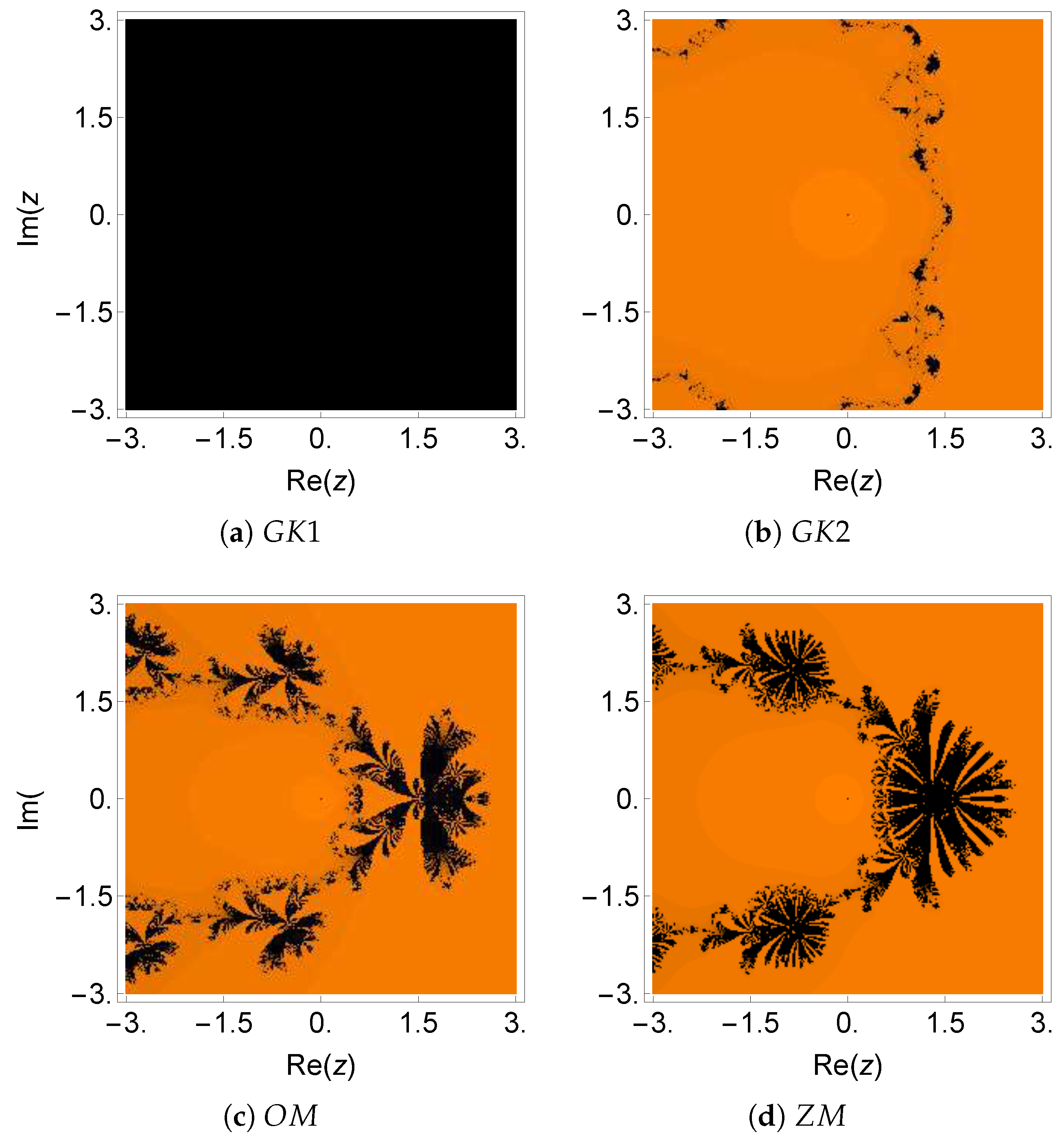
We observed that all methods converged only if the initial guess was chosen sufficiently close to the desired root. Therefore, going a step further, we decided to investigate the dynamical behavior of the test functions $f_i\left(x\right),i=1,2,\cdots ,7,$ in the complex plane. In other words, we numerically approximated the domain of attraction of the zeros as a qualitative measure of how the methods depend on the choice of the initial approximation of the root. To answer this important question on the behavior of the algorithms, we discussed the complex dynamics of the iterative maps (32), (33), and (35) and compared them with the schemes (36), (37), (5), and (6), respectively.

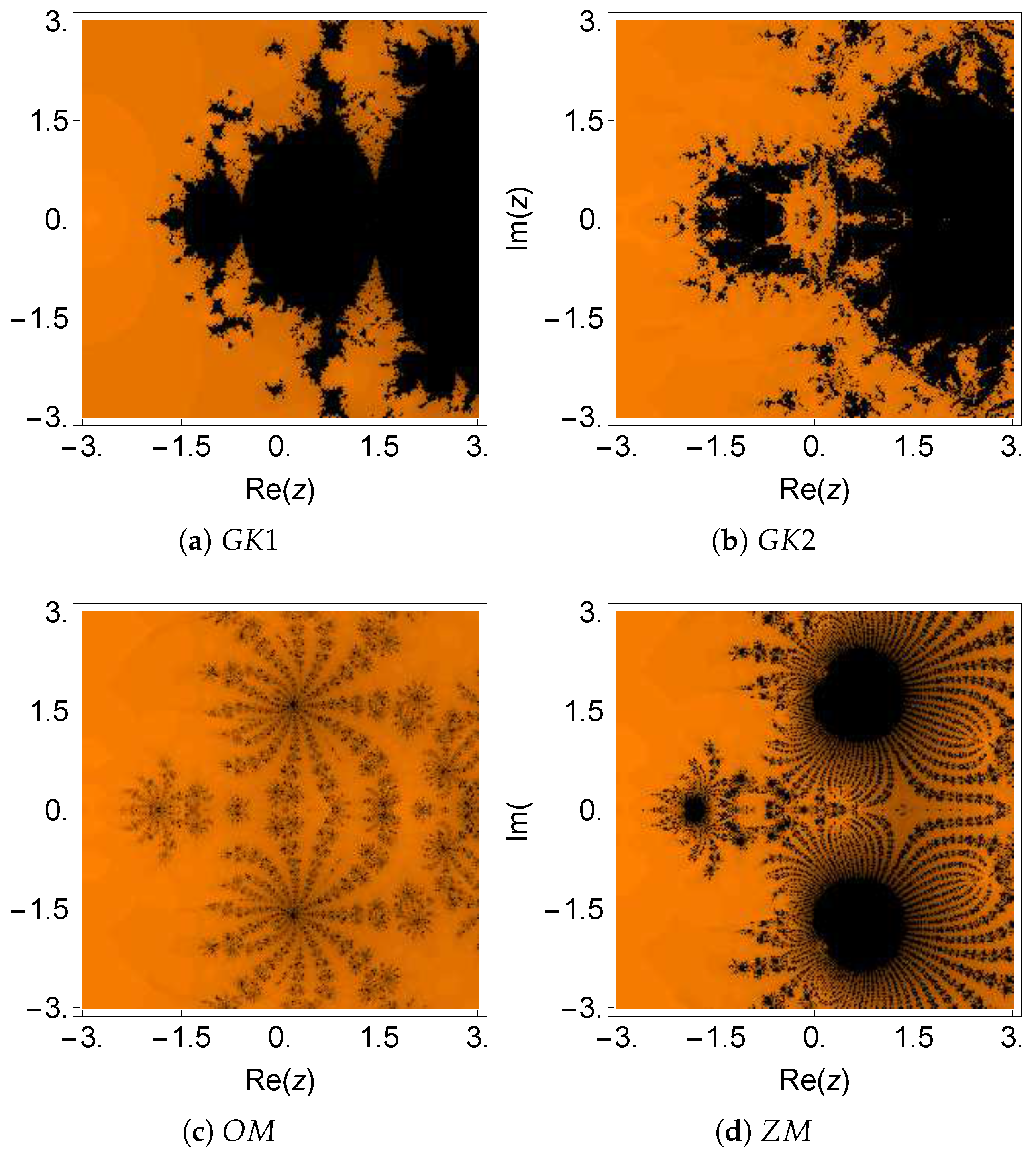
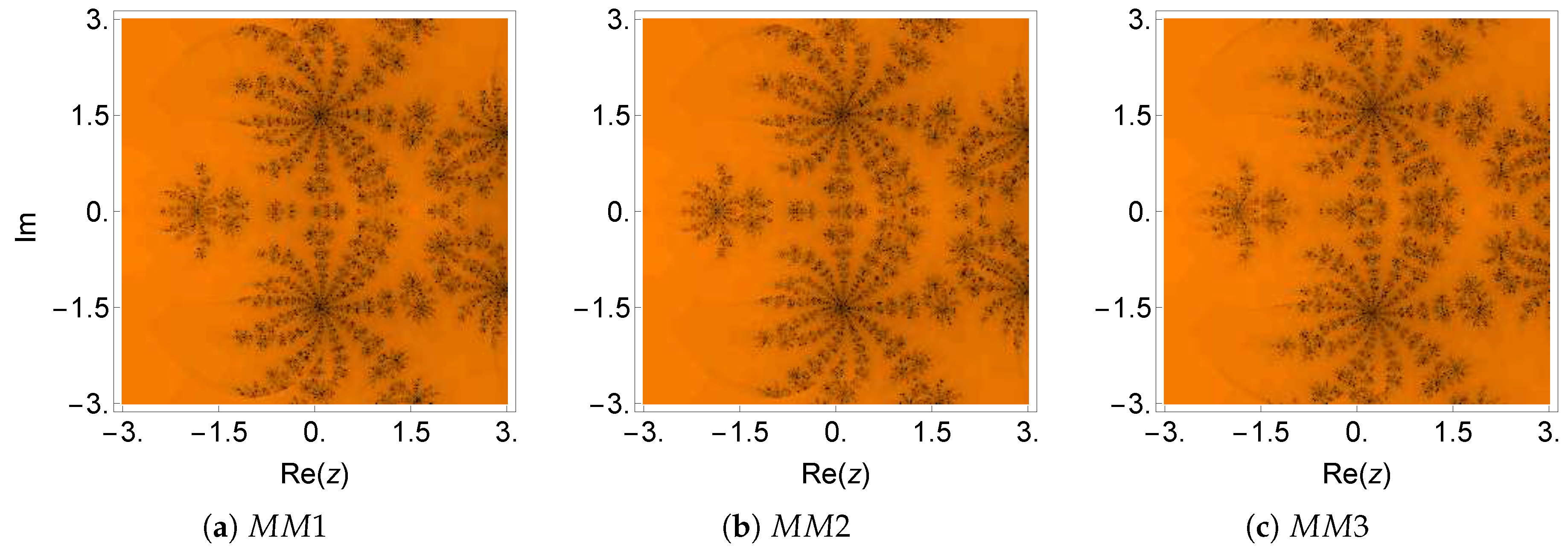
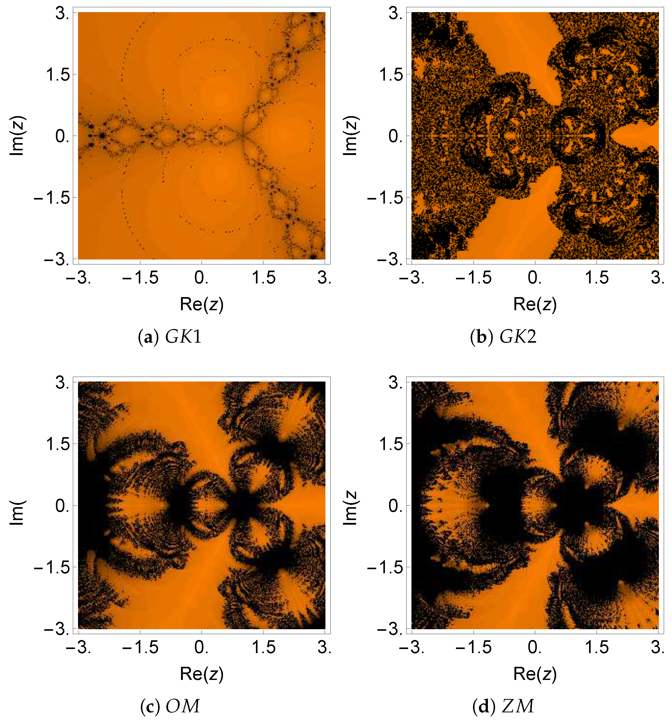
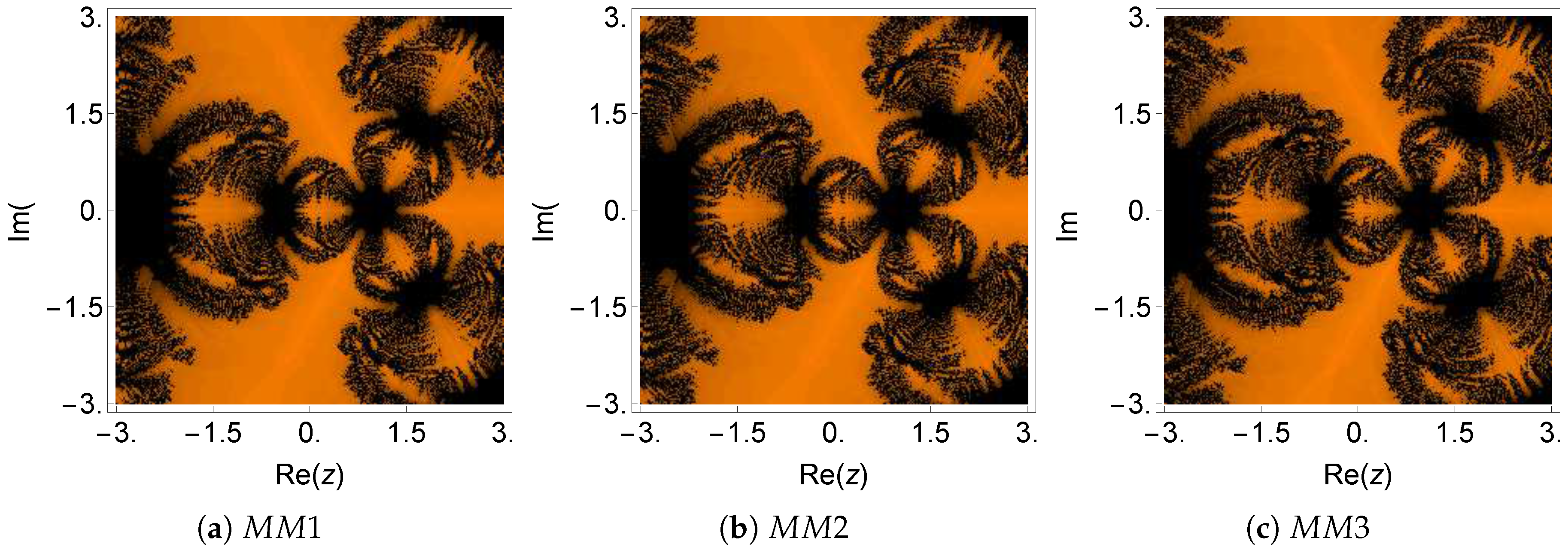
From the dynamical and graphical point of view [23,24], we took a $600\times 600$ grid of the square $[-3,3]\times [-3,3]\in \mathbb{C}$ and assigned orange color to those points whose orbits converged to the multiple root. We represent a given point as black if the orbit converges to strange fixed points or diverges after at most 25 iterations using a tolerance of ${10}^{-3}$. Note that the black color denotes lack of convergence of the algorithm to any of the roots. This happened, in particular, when the method converged to a strange fixed point (fixed points that were not roots of the nonlinear function), ended in a periodic cycle, or went to infinity.

Table 8. Measures of convergence of the seven iterative methods for test functions $f_i\left(x\right)=0$, $i=1,\dots ,7$.

$\mathit{f}\left(\mathit{x}\right)$	Methods	I/P	NC (%)	${\mathit{I}}_{\mathit{C}}/\mathit{C}$	$\mathit{f}\left(\mathit{x}\right)$	Methods	I/P	NC (%)	${\mathit{I}}_{\mathit{C}}/\mathit{C}$
$f_1\left(x\right)$	$GK1$	14.82	38.57	8.43	$f_5\left(x\right)$	$GK1$	0.99	99.99	0.00
	$GK2$	12.06	36.09	4.75		$GK2$	2.54	1.40	2.30
	$OM$	6.79	0.12	6.77		$OM$	4.86	12.32	2.84
	$ZM$	11.08	9.15	9.67		$ZM$	4.55	15.36	2.58
	$MM1$	5.95	0.04	5.95		$MM1$	5.17	12.41	2.92
	$MM2$	5.99	0.03	5.99		$MM2$	5.19	12.62	2.90
	$MM3$	6.60	0.04	6.59		$MM3$	5.22	12.50	2.98
$f_2\left(x\right)$	$GK1$	1.00	100	6.32	$f_6\left(x\right)$	$GK1$	3.48	0.00	3.48
	$GK2$	8.93	99.58	1.6		$GK2$	3.52	0.00	3.52
	$OM$	11.05	99.99	1.6		$OM$	3.25	0.00	3.25
	$ZM$	10.23	99.98	2.15		$ZM$	3.52	0.01	3.53
	$MM1$	11.72	99.99	1.6		$MM1$	3.32	0.00	3.32
	$MM2$	11.87	99.99	1.6		$MM2$	3.32	0.00	3.32
	$MM3$	11.82	99.99	1.6		$MM3$	3.32	0.00	3.32
$f_3\left(x\right)$	$GK1$	13.71	42.03	5.52	$f_7\left(x\right)$	$GK1$	1	100	$**$
	$GK2$	12.18	38.63	4.11		$GK2$	1	0	1
	$OM$	7.29	1.13	7.09		$OM$	1	0	1
	$ZM$	12.50	22.31	8.91		$ZM$	1	0	1
	$MM1$	6.97	0.71	6.84		$MM1$	1	0	1
	$MM2$	6.99	0.63	6.88		$MM2$	1	0	1
	$MM3$	6.84	0.62	6.73		$MM3$	1	0	1
$f_4\left(x\right)$	$GK1$	6.78	1.25	6.55
	$GK2$	16.05	45.88	8.47
	$OM$	15.77	40.18	9.58
	$ZM$	17.74	56.04	8.52
	$MM1$	15.64	39.12	9.63
	$MM2$	15.67	39.16	9.67
	$MM3$	16.41	42.22	10.13

** stands for indeterminate.

depicts the measures of convergence of different iterative methods in terms of the average number of iterations per point. The column $I/P$ shows the average number of iterations per point until the algorithm decided that a root had been reached, otherwise it indicates that the point was non-convergent. The column $NC(\%)$ shows the percentage of non-convergent points, indicated as black zones in the fractal pictures represented in Figure 1, Figure 2, Figure 3, Figure 4, Figure 5, Figure 6, Figure 7, Figure 8, Figure 9, Figure 10, Figure 11, Figure 12, Figure 13 and Figure 14. It is clear that the non-convergent points had a considerable influence on the values of $I/P$ since these points contributed always with the maximum number of 25 allowed iterations. In contrast, convergent points were reached usually very quickly because we were working with multipoint iterative methods of higher order. Therefore, to minimize the effect of non-convergent points, we included the column $I_C/C$, which shows the average number of iterations per convergent point.

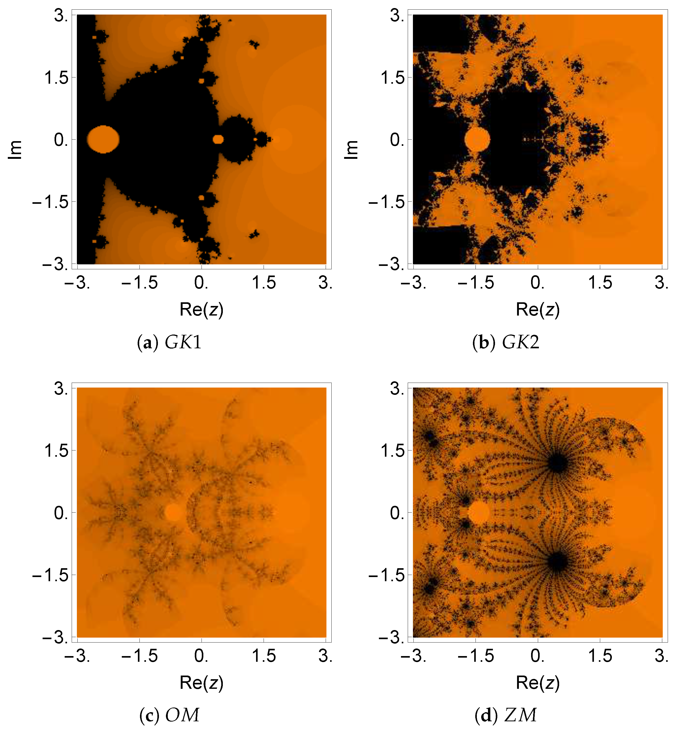
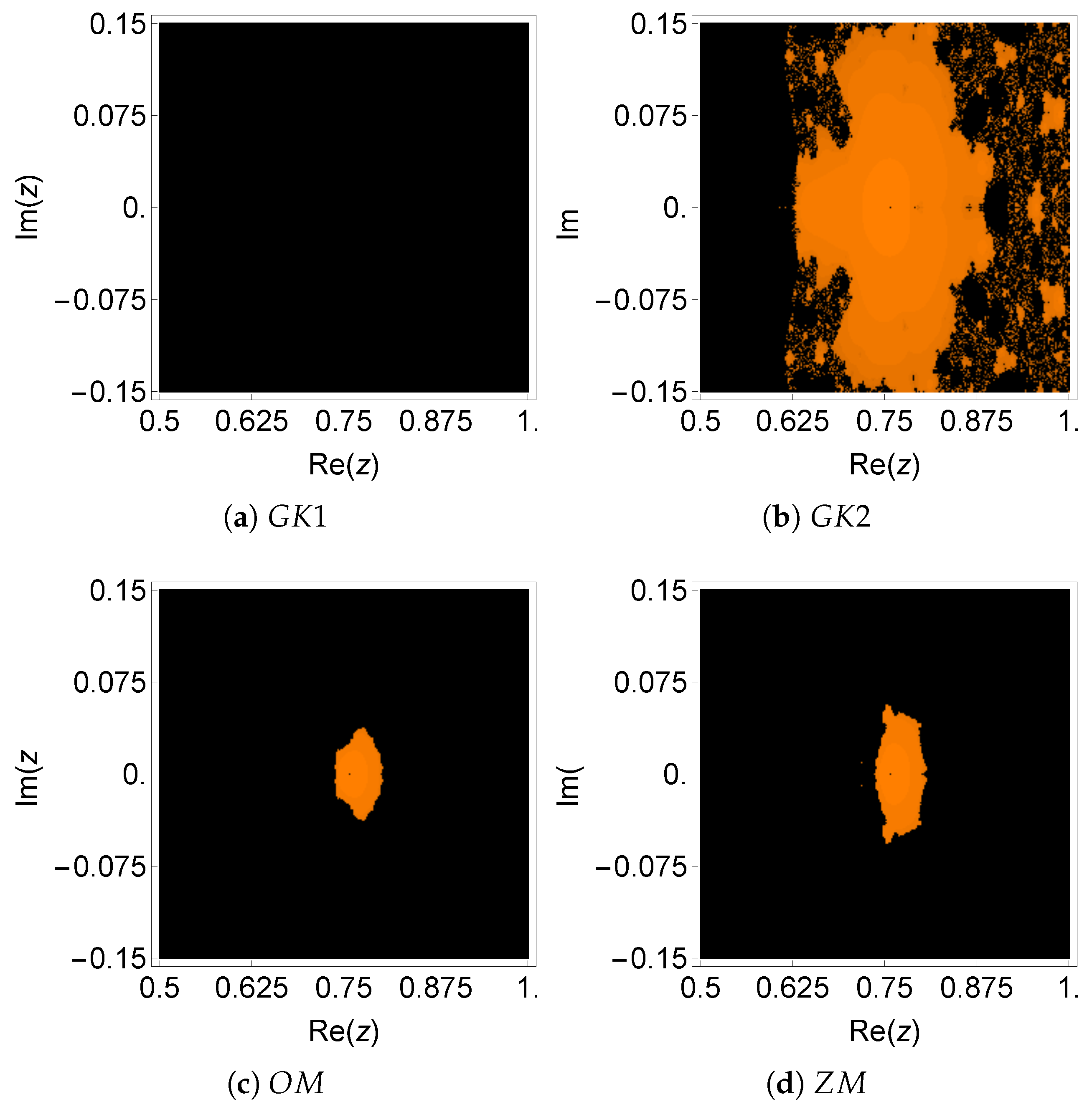
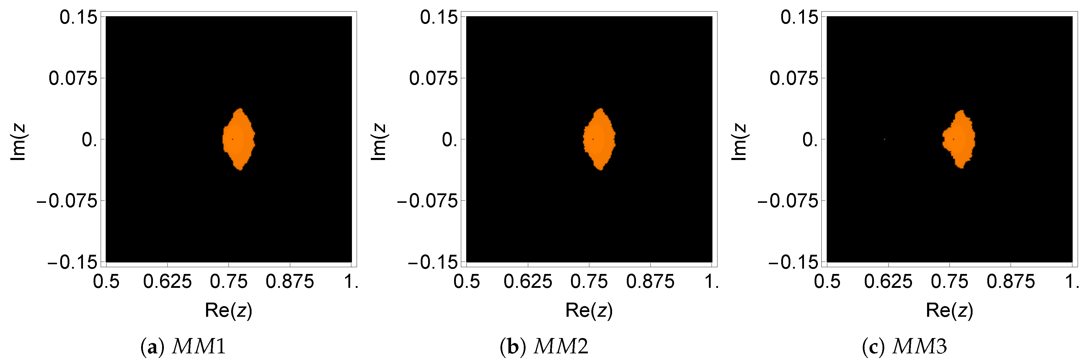
Example 1.

We considered the van der Waals equation of state [25]:

$$\left(P+\frac{a{n}^2}{V^2}\right)(V-nb)=nRT,$$

where a and b explain the behavior of a real gas by introducing in the ideal equations two parameters, a and b (known as van der Waals constants), specific for each case. The determination of the volume V of the gas in terms of the remaining parameters required the solution of a nonlinear equation in V:

$$P{V}^3-(nbP+nRT)V^2+a{n}^{2}V-ab{n}^2=0.$$

Given the constants a and b that characterize a particular gas, one can find values for n, P, and T, such that this equation has three roots. By using the particular values, we obtained the following nonlinear function (see [26] for more details)

$$f_1\left(x\right)=x^3-5.22x^2+9.0825x-5.2675,$$

having three zeros, so that one is $x=1.75$, of multiplicity of two, and the other $x=1.72$. However, our desired root was $x=1.75$.

The numerical results shown in Table 1 reveal that the new methods $MM1$, $MM2$, and $MM3$ had better performance than the others in terms of precision in the calculation of the multiple roots of $f_1\left(x\right)=0$. On the other hand, the dynamical planes of different iterative methods for this problem are given in Figure 1 and Figure 2. One can see that the new methods had a larger stable (area marked in orange) than the methods $GK1$, $GK2$, $OM$, and $ZM$. It can also be verified from Table 8 that the three new methods required a smaller average number of iterations per point ($I/P$) and a smaller percentage of non-convergent points ($NC(\%)$). Furthermore, we found that $MM1$ used the smallest number of iterations per point ($I/P=$5.95 on average), while $GK1$ required the highest number of iterations per point ($I/P=$14.82).

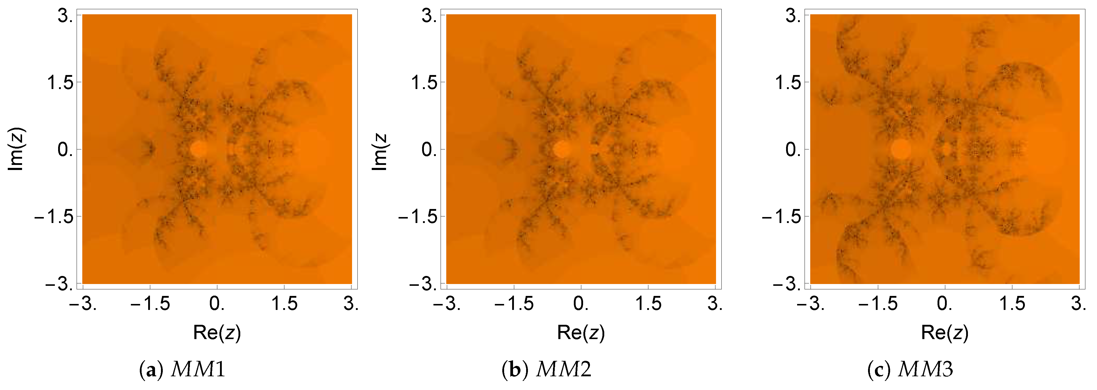
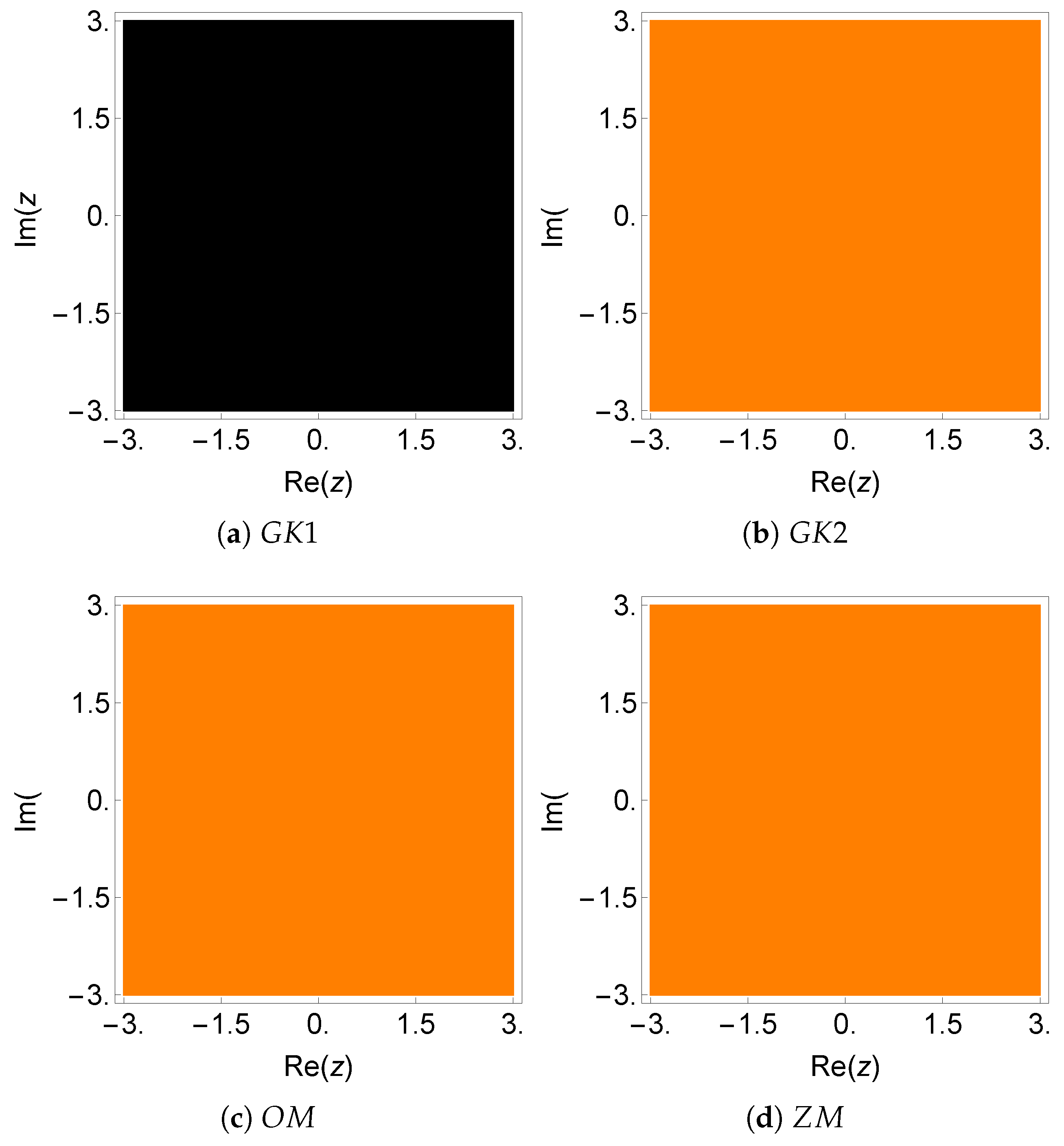
Example 2.

Fractional conversion in a chemical reactor:

Let us consider the following equation (see [27,28] for more details):

$$f_2\left(x\right)=\frac{x}{1-x}-5log\left[\frac{0.4(1-x)}{0.4-0.5x}\right]+4.45977.$$

(38)

In the above equation, x represents the fractional conversion of Species A in a chemical reactor. There is no physical meaning of Equation (38) if x is less than zero or greater than one, since x is bounded in the region $0\le x\le 1$. The required zero (that is simple) to this problem is $x\approx 0.757396246253753879459641297929$. Nonetheless, the above equation is undefined in the region $0.8\le x\le 1$, which is very close to the desired zero. Furthermore, there are some other properties of this function that make the solution more difficult to obtain. In fact, the derivative of the above equation is very close to zero in the region $0\le x\le 0.5$, and there is an infeasible solution for $x=1.098$.

From Figure 3 and Figure 4, we verified that the basin of attraction of the searched root (orange color) was very small, or does not exist in most of the methods. The number of non-convergent points that corresponds to the black area was very large for all the considered methods (see Table 8). Moreover, an almost symmetric orange-colored area appeared in some cases, which corresponds to the solution without physical sense, that is an attracting fixed point. Except for $GK1$ (not applicable for simple roots), all other methods converged to the multiple roost only if the initial guess was chosen sufficiently close to the required root, although the basins of attraction were quite small in all cases. The numerical results presented in Table 2 are compatible with the dynamical results in Figure 3 and Figure 4. We can see that the new methods revealed smaller residual error and a smaller difference between the consecutive approximations in comparison to the existing ones. Moreover, the numerical estimation of the order of convergence coincided with the theoretical one in all cases. In Table 2, the symbol * means that the corresponding method does not converge to the desired root.

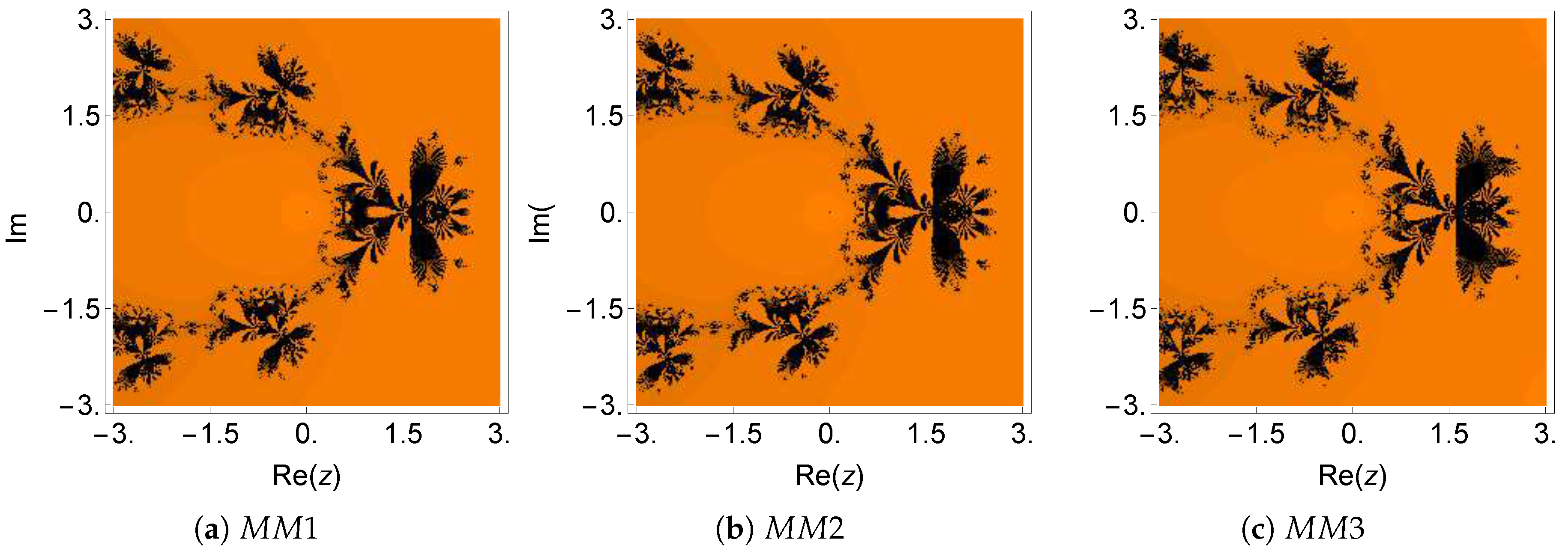
Example 3.

Continuous stirred tank reactor (CSTR) [20,29]:

In this third example, we considered the isothermal continuous stirred tank reactor (CSTR) problem. The following reaction scheme develops in the reactor (see [30] for more details):

$$\begin{array}{c}A+R\to B\hfill \\ B+R\to C\hfill \\ C+R\to D\hfill \\ C+R\to E,\hfill \end{array}$$

(39)

where components A and R are fed to the reactor at rates of Q and $q-Q$, respectively. The problem was analyzed in detail by Douglas [31] in order to design simple feedback control systems. In the modeling study, the following equation for the transfer function of the reactor was given:

$$\begin{array}{c}\hfill K_C{\displaystyle \frac{2.98(x+2.25)}{(s+1.45){(s+2.85)}^2(s+4.35)}}=-1,\end{array}$$

(40)

where $K_C$ is the gain of the proportional controller. The control system is stable for values of $K_C$, which yields roots of the transfer function having a negative real part. If we choose $K_C=0$, then we get the poles of the open-loop transfer function as roots of the nonlinear equation:

$$\begin{array}{c}\hfill f_3\left(x\right)=x^4+11.50x^3+47.49x^2+83.06325x+51.23266875=0\end{array}$$

(41)

such as $x=-1.45$, $-2.85$, $-2.85$, $-4.35$. Therefore, we see that there is one root $x=-2.85$ with multiplicity two.

The numerical results for this example are listed in Table 3. The dynamical planes for this example are plotted in Figure 5 and Figure 6. For methods $GK1$, $GK2$, and $ZM$, the black region of divergence was very large, which means that the methods would not converge if the initial point was located inside this region. This effect can also be observed from Table 8, where the average number of iterations per point and percentage of non-convergent points are high for methods $GK1$ ($I/P=$ 13.71 on average), $GK2$ ($I/P=$ 12.18 on average), and $ZM$ ($I/P=$ 12.50 on average), while the new methods have a comparatively smaller number of iterations per point. The results of method $OM$ closely follow the new methods with an average number of 7.29 iterations per point.

Example 4.

Let us consider another nonlinear test function from [2], as follows:

$$f_4\left(x\right)={({(x-1)}^3-1)}^{50}.$$

The above function has a multiple zero at $x=2$ of multiplicity 50.

Table 4 shows the numerical results for this example. It can be observed that the results were very good for all the cases, the residuals being lower for the newly-proposed methods. Moreover, the asymptotic error constant ($\eta$) displayed in the last column of Table 4 was large for the methods $OM$ and $ZM$ in comparison to the other schemes. Based on the dynamical planes in Figure 7 and Figure 8, it is observed that in all schemes, except $GK1$, the black region of divergence was very large. This is also justified from the observations of Table 8. We verified that $ZM$ required the highest average number of iterations per point ($I/P=$ 17.74), while $GK1$ required the smallest number of iterations per point ($I/P=$6.78). All other methods required an average number of iterations per point in the range of 15.64–16.67. Furthermore, we observed that the percentage of non-convergent points $NC(\%)$ was very high for $ZM$ ($56.04\%$) followed by $GK2$ ($45.88\%$). Furthermore, it can also be seen that the average number of iterations per convergent point ($I_C/C$) for the methods $GK1$, $GK2$, $OM$, and $ZM$ was 6.55, 8.47, 9.58, and 8.52, respectively. On the other hand, the proposed methods $MM1$, $MM2$, and $MM3$ required 9.63, 9.67, and 10.13, respectively.

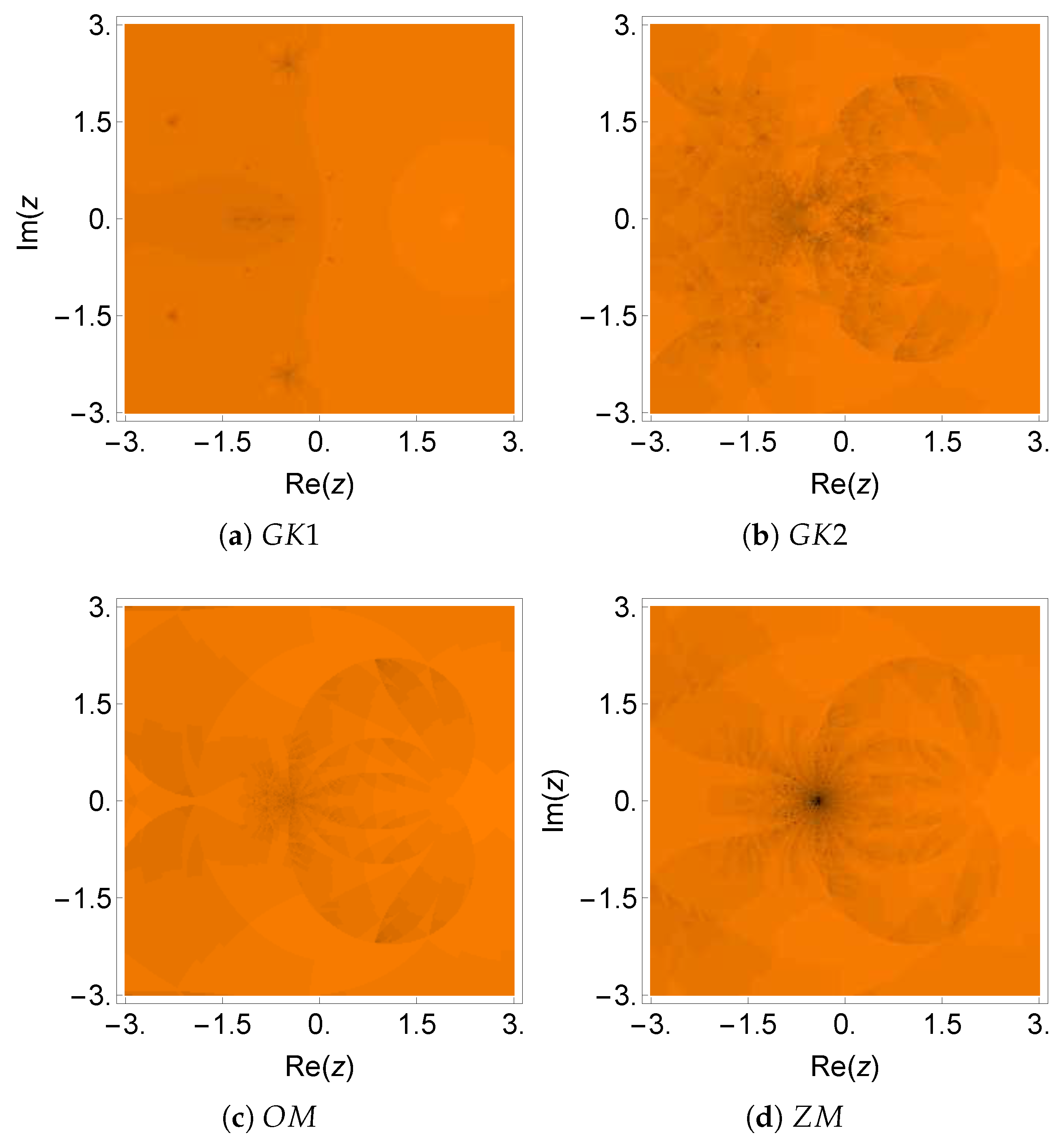
Example 5.

Planck’s radiation law problem [32]:

We considered the following Planck’s radiation law problem that calculates the energy density within an isothermal blackbody and is given by [33]:

$$\Psi \left(\lambda \right)={\displaystyle \frac{8\pi ch{\lambda }^{-5}}{e^{\frac{ch}{\lambda BT}}-1}},$$

(42)

where λ represents the wavelength of the radiation, T stands for the absolute temperature of the blackbody, B is the Boltzmann constant, h denotes Planck’s constant, and c is the speed of light. We were interested in determining the wavelength λ that corresponds to the maximum energy density $\Psi \left(\lambda \right)$.

The condition ${\Psi }^{\prime }\left(\lambda \right)=0$ implies that the maximum value of Ψ occurs when:

$${\displaystyle \frac{\frac{ch}{\lambda BT}{e}^{\frac{ch}{\lambda BT}}}{e^{\frac{ch}{\lambda BT}}-1}}=5.$$

(43)

If $x=\frac{ch}{\lambda BT}$, then (43) is satisfied when:

$$f_5\left(x\right)=e^{-x}+\frac{x}{5}-1=0.$$

(44)

Therefore, the solutions of $f_5\left(x\right)=0$ give the maximum wavelength of radiation λ by means of the following formula:

$$\lambda \approx \frac{ch}{\alpha BT},$$

(45)

where α is a solution of (44). The desired root is $x=4.9651142317442$ with multiplicity $m=1$.

The numerical results for the test equation $f_5\left(x\right)=0$ are displayed in Table 5. It can be observed that $MM1$ and $MM2$ had small values of residual errors and asymptotic error constants ($\eta$), in comparison to the other methods, when the accuracy was tested in multi-precision arithmetic. Furthermore, the basins of attraction for all the methods are represented in Figure 9 and Figure 10. One can see that the fractal plot of the method $GK1$ was completely black because the multiplicity of the desired root was unity in this case. On the other hand, method $GK2$ had the most reduced black area in Figure 9b, which is further justified in Table 8. The method $GK2$ had a minimum average number of iterations per point ($I/P=$ 2.54) and the smallest percentage of non-convergent points ($1.40\%$), while $ZM$ had the highest percentage of non-convergent points ($15.36\%$). For the other methods, the average number of iterations per point was in the range from 4.55–5.22 and the percentage of non-convergent points lies between 12.32 and 12.62.

Example 6.

Consider the following $5\times 5$ matrix [29]:

$$B=\left[\begin{array}{ccccc}29& 14& 2& 6& -9\\ -47& -22& -1& -11& 13\\ 19& 10& 5& 4& -8\\ -19& -10& -3& -2& 8\\ 7& 4& 3& 1& -3\end{array}\right].$$

The corresponding characteristic polynomial of this matrix is as follows:

$$f_6\left(x\right)={(x-2)}^4(x+1).$$

(46)

The characteristic equation has one root at $x=2$ of multiplicity four.

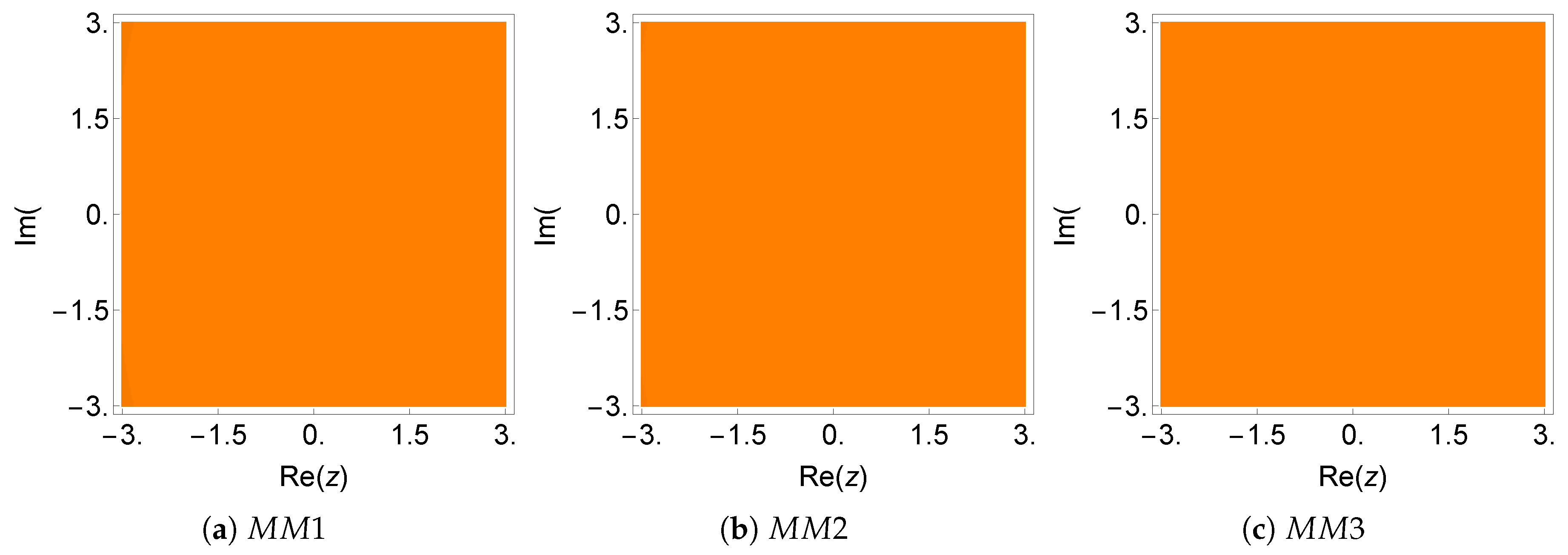
Table 6 shows the numerical results for this example. It can be observed in Figure 11 and Figure 12 that the orange areas dominate the plot. In fact, they correspond to the basin of attraction of the searched zero. This means that the method converges if the initial estimation was located inside this orange region. All schemes had a negligible black portion, as can be observed in Figure 11 and Figure 12. Moreover, the numerical tests for this nonlinear function showed that $MM1$, $MM2$, and $MM3$ had the best results in terms of accuracy and estimation of the order of convergence. Consulting Table 8, we note that the average number of iterations per point ($I/P$) was almost identical for all methods (ranging from 3.25–3.52).

Example 7.

Global CO${}_2$ model by McHugh et al. [34] in ocean chemistry:

In this example, we discuss the global CO${}_2$ model by McHugh et al. [34] in ocean chemistry (please see [35] for more details). This problem leads to the numerical solution of a nonlinear fourth-order polynomial in the calculation of $pH$ of the ocean. The effect of atmospheric CO${}_2$ is very complex and varies with the location. Therefore, Babajee [35] considered a simplified approach based on the following assumptions:

1. 

Only the ocean upper layer is considered (not the deep layer),

2. 

Neglecting the spatial variations, an approximation of the ocean upper layer carbon distribution by perfect mixing is considered.

As the CO${}_2$ dissolves in ocean water, it undergoes a series of chemical changes that ultimately lead to increased hydrogen ion concentration, denoted as $\left[H^{+}\right]$, and thus acidification. The problem was analyzed by Babajee [35] in order to find the solution of the following nonlinear function:

$$p\left(\left[H^{+}\right]\right)=\sum _{n=0}^4{\delta }_n{\left[H^{+}\right]}^n,$$

(47)

so that:

$$\left\{\begin{array}{c}{\delta }_0=2N_0{N}_1{N}_2{P}_t{N}_B,\hfill \\ {\delta }_1=N_0{N}_1{P}_t{N}_B+2N_0{N}_1{N}_2{P}_t+N_W{N}_B,\hfill \\ {\delta }_2=N_0{N}_1{P}_t+B{N}_B+N_W-A{N}_B,\hfill \\ {\delta }_3=-N_B-A,\hfill \\ {\delta }_4=-1.\hfill \end{array}\right.$$

(48)

where $N_0,N_1,N_2,N_W$, and $N_B$ are equilibrium constants. The parameter A represents the alkalinity, which expresses the neutrality of the ocean water, and $P_t$ is the gas phase CO${}_2$ partial pressure. We assume the values of $A=2.050$ and $B=0.409$ taken by Sarmiento and Gruyber [36] and Bacastow and Keeling [37], respectively. Furthermore, choosing the values of $N_0,N_1,N_2,N_W$, $N_B$ and $P_t$ given by Babajee [35], we obtain the following nonlinear equation:

$$f_7\left(x\right)=x^4-\frac{2309x^3}{250}-\frac{65226608163x^2}{500000}+\frac{425064009069x}{25000}-\frac{10954808368405209}{62500000}=0.$$

(49)

The roots of $f_7\left(x\right)=0$ are given by $x=-411.452,11.286,140.771,268.332$. Hereafter, we pursue the root $-411.452$ having multiplicity $m=1$.

The numerical experiments of this example are given in Table 7. The methods $MM1$, $MM2$, and $MM3$ had small residual errors and asymptotic error constants when compared to the other schemes. The computational order of convergence for all methods coincided with the theoretical ones in seven cases. Figure 13 and Figure 14 show the dynamical planes of all the methods on test function $f_7\left(x\right)$. It can be observed that all methods showed stable behavior, except $GK1$, as can also be confirmed in Table 8.

4. Conclusions

This paper developed a wide general three-step class of methods for approximating multiple zeros of nonlinear functions numerically. Optimal iteration schemes having eighth order for multiple zeros have been seldom considered in the literature. Therefore, the presented methods may be regarded as a further step in this area. Weight functions based on function-to-function ratios and free parameters were employed in the second and third steps of the family. This strategy allowed us to achieve the desired convergence order of eight. In the numerical section, we considered a large variety of real-life problems. The seven examples confirmed the efficiency of the proposed technique in comparison to the existing robust methods. From the computational results, we found that the new methods showed superior performance in terms of precision, the average number of iterations per point, and the percentage of non-convergent points for the considered seven test functions. The straightforward structure and high convergence order of the proposed class make it relevant both from the theoretical and practical points of view.

References

1. Traub, J.F. Iterative Methods for the Solution of Equations; Prentice-Hall: Englewood Cliffs, NJ, USA, 1964. [Google Scholar]
2. Petković, M.S.; Neta, B.; Petković, L.D.; Džunić, J. Multipoint Methods for Solving Nonlinear Equations; Academic Press: Cambridge, MA, USA, 2013. [Google Scholar]
3. Abad, M.F.; Cordero, A.; Torregrosa, J.R. Fourth-and fifth-order methods for solving nonlinear systems of equations: An application to the global positioning system. Abstr. Appl. Anal. 2013, 2013. [Google Scholar] [CrossRef]
4. Farhane, N.; Boumhidi, I.; Boumhidi, J. Smart Algorithms to Control a Variable Speed Wind Turbine. Int. J. Interact. Multimed. Artif. Intell. 2017, 4, 88–95. [Google Scholar] [CrossRef]
5. Abdel-Nasser, M.; Mahmoud, K.; Kashef, H. A Novel Smart Grid State Estimation Method Based on Neural Networks. Int. J. Interact. Multimed. Artif. Intell. 2018, 5, 92–100. [Google Scholar] [CrossRef]
6. Arora, S.; Singh, S. An Effective Hybrid Butterfly Optimization Algorithm with Artificial Bee Colony for Numerical Optimization. Int. J. Interact. Multimed. Artif. Intell. 2017, 4, 14–21. [Google Scholar] [CrossRef]
7. Ostrowski, A.M. Solution of Equations and Systems of Equations; Academic Press: New York, NY, USA, 1960. [Google Scholar]
8. Behl, R.; Cordero, A.; Motsa, S.S.; Torregrosa, J.R. On developing fourth-order optimal families of methods for multiple roots and their dynamics. Appl. Math. Comput. 2015, 265, 520–532. [Google Scholar] [CrossRef] [Green Version]
9. Behl, R.; Cordero, A.; Motsa, S.S.; Torregrosa, J.R.; Kanwar, V. An optimal fourth-order family of methods for multiple roots and its dynamics. Numer. Algor. 2016, 71, 775–796. [Google Scholar] [CrossRef]
10. Li, S.; Liao, X.; Cheng, L. A new fourth-order iterative method for finding multiple roots of nonlinear equations. Appl. Math. Comput. 2009, 215, 1288–1292. [Google Scholar]
11. Neta, B.; Chun, C.; Scott, M. On the development of iterative methods for multiple roots. Appl. Math. Comput. 2013, 224, 358–361. [Google Scholar] [CrossRef] [Green Version]
12. Sharma, J.R.; Sharma, R. Modified Jarratt method for computing multiple roots. Appl. Math. Comput. 2010, 217, 878–881. [Google Scholar] [CrossRef]
13. Zhou, X.; Chen, X.; Song, Y. Constructing higher-order methods for obtaining the multiple roots of nonlinear equations. J. Comput. Appl. Math. 2011, 235, 4199–4206. [Google Scholar] [CrossRef] [Green Version]
14. Li, S.; Cheng, L.; Neta, B. Some fourth-order nonlinear solvers with closed formulae for multiple roots. Comput. Math. Appl. 2010, 59, 126–135. [Google Scholar] [CrossRef] [Green Version]
15. Neta, B. Extension of Murakami’s high-order non-linear solver to multiple roots. Int. J. Comput. Math. 2010, 87, 1023–1031. [Google Scholar] [CrossRef]
16. Thukral, R. Introduction to higher-order iterative methods for finding multiple roots of nonlinear equations. J. Math. 2013, 2013. [Google Scholar] [CrossRef]
17. Geum, Y.H.; Kim, Y.I.; Neta, B. A class of two-point sixth-order multiple-zero finders of modified double-Newton type and their dynamics. Appl. Math. Comput. 2015, 270, 387–400. [Google Scholar] [CrossRef] [Green Version]
18. Geum, Y.H.; Kim, Y.I.; Neta, B. A sixth-order family of three-point modified Newton-like multiple-root finders and the dynamics behind their extraneous fixed points. Appl. Math. Comput. 2016, 283, 120–140. [Google Scholar] [CrossRef] [Green Version]
19. Behl, R.; Cordero, A.; Motsa, S.S.; Torregrosa, J.R. An eighth-order family of optimal multiple root finders and its dynamics. Numer. Algor. 2018, 77, 1249–1272. [Google Scholar] [CrossRef]
20. Zafar, F.; Cordero, A.; Quratulain, R.; Torregrosa, J.R. Optimal iterative methods for finding multiple roots of nonlinear equations using free parameters. J. Math. Chem. 2017. [Google Scholar] [CrossRef]
21. Artidiello, S.; Cordero, A.; Torregrosa, J.R.; Vassileva, M.P. Two weighted eight-order classes of iterative root-finding methods. Int. J. Comput. Math. 2015, 92, 1790–1805. [Google Scholar] [CrossRef]
22. Jay, L.O. A note on Q-order of convergence. BIT Numer. Math. 2001, 41, 422–429. [Google Scholar] [CrossRef]
23. Varona, J.L. Graphic and numerical comparison between iterative methods. Math. Intell. 2002, 24, 37–46. [Google Scholar] [CrossRef]
24. Matthies, G.; Salimi, M.; Varona, J.L.; Sharifi, S. An optimal three-point eighth-order iterative method without memory for solving nonlinear equations with its dynamics. Jpn. J. Ind. Appl. Math. 2016, 33, 751–766. [Google Scholar] [CrossRef] [Green Version]
25. Behl, R.; Alshomrani, A.S.; Motsa, S.S. An optimal scheme for multiple roots of nonlinear equations with eighth-order convergence. J. Math. Chem. 2018, 56, 2069–2084. [Google Scholar] [CrossRef]
26. Hueso, J.L.; Martínez, E.; Teruel, C. Determination of multiple roots of nonlinear equations and applications. J. Math. Chem. 2015, 53, 880–892. [Google Scholar] [CrossRef]
27. Magreñán, Á.A.; Argyros, I.K.; Rainer, J.J.; Sicilia, J.A. Ball convergence of a sixth-order Newton-like method based on means under weak conditions. J. Math. Chem. 2018, 56, 2117–2131. [Google Scholar] [CrossRef]
28. Shacham, M. Numerical solution of constrained nonlinear algebraic equations. Int. J. Numer. Method Eng. 1986, 23, 1455–1481. [Google Scholar] [CrossRef]
29. Kansal, M.; Behl, R.; Mahnashi, M.A.A.; Mallawi, F.O. Modified Optimal Class of Newton-Like Fourth-Order Methods for Multiple Roots. Symmetry 2019, 11, 526. [Google Scholar] [CrossRef]
30. Constantinides, A.; Mostoufi, N. Numerical Methods for Chemical Engineers with MATLAB Applications; Prentice Hall PTR: Englewood Cliffs, NJ, USA, 1999. [Google Scholar]
31. Douglas, J.M. Process Dynamics and Control; Prentice Hall: Englewood Cliffs, NJ, USA, 1972; Volume 2. [Google Scholar]
32. Maroju, P.; Magreñán, Á.A.; Motsa, S.S. Second derivative free sixth order continuation method for solving nonlinear equations with applications. J. Math. Chem. 2018, 56, 2099–2116. [Google Scholar] [CrossRef]
33. Jain, D. Families of Newton-like method with fourth-order convergence. Int. J. Comput. Math. 2013, 90, 1072–1082. [Google Scholar] [CrossRef]
34. McHugh, A.J.; Griffiths, G.W.; Schiesser, W.E. An Introductory Global CO2 Model: (with Companion Media Pack); World Scientific Pub Co Inc: Singapore, 2015. [Google Scholar]
35. Babajee, D.K.R. Analysis of Higher Order Variants of Newton’s Method and Their Applications to Differential and Integral Equations and in Ocean Acidification. Ph.D. Thesis, University of Mauritius, Moka, Mauritius, 2010. [Google Scholar]
36. Sarmiento, J.L.; Gruber, N. Ocean Biogeochemical Dynamics; Princeton University Press: Princeton, NJ, USA, 2006. [Google Scholar]
37. Bacastow, R.; Keeling, C.D. Atmospheric carbon dioxide and radiocarbon in the natural carbon cycle: Changes from a.d. 1700 to 2070 as deduced from a geochemical model. In Proceedings of the 24th Brookhaven Symposium in Biology; Woodwell, G.W., Pecan, E.V., Eds.; The Technical Information Center, Office of Information Services, United State Atomic Energy Commission: Upton, NY, USA, 1972; pp. 86–133. [Google Scholar]
Figure 1. Dynamical plane of the methods G K 1 , G K 2 , O M , and Z M on f 1 ( x ) .
Symmetry 11 00837 g001
Figure 2. Dynamical plane of the methods M M 1 , M M 2 , and M M 3 on f 1 ( x ) .
Symmetry 11 00837 g002
Figure 3. Dynamical plane of the methods G K 1 , G K 2 , O M , and Z M on f 2 ( x ) .
Symmetry 11 00837 g003
Figure 4. Dynamical plane of the methods M M 1 , M M 2 , and M M 3 on f 2 ( x ) .
Symmetry 11 00837 g004
Figure 5. Dynamical plane of the methods G K 1 , G K 2 , O M , and Z M on f 3 ( x ) .
Symmetry 11 00837 g005
Figure 6. Dynamical plane of the methods M M 1 , M M 2 , and M M 3 on f 3 ( x ) .
Symmetry 11 00837 g006
Figure 7. Dynamical plane of the methods G K 1 , G K 2 , O M , and Z M on f 4 ( x ) .
Symmetry 11 00837 g007
Figure 8. Dynamical plane of the methods M M 1 , M M 2 , and M M 3 on f 4 ( x ) .
Symmetry 11 00837 g008
Figure 9. Dynamical plane of the methods G K 1 , G K 2 , O M , and Z M on f 5 ( x ) .
Symmetry 11 00837 g009
Figure 10. Dynamical plane of the methods M M 1 , M M 2 , and M M 3 on f 5 ( x ) .
Symmetry 11 00837 g010
Figure 11. Dynamical plane of the methods G K 1 , G K 2 , O M , and Z M on f 6 ( x ) .
Symmetry 11 00837 g011
Figure 12. Dynamical plane of the methods M M 1 , M M 2 , and M M 3 on f 6 ( x ) .
Symmetry 11 00837 g012
Figure 13. Dynamical plane of the methods G K 1 , G K 2 , O M , and Z M on f 7 ( x ) .
Symmetry 11 00837 g013
Figure 14. Dynamical plane of the methods M M 1 , M M 2 , and M M 3 on f 7 ( x ) .
Symmetry 11 00837 g014