Finite Element Modelling of a Composite Shell with Shear Connectors

Abstract

A three-layer composite shell with shear connectors is made of three shell layers with one another connected by stubs at the contact surfaces. These layers can have similar or different geometrical and physical properties with the assumption that they always contact and have relative movement in the working process. Due to these characteristics, they are used widely in many engineering applications, such as ship manufacturing and production, aerospace technologies, transportation, and so on. However, there are not many studies on these types of structures. This paper is based on the first-order shear deformation Mindlin plate theory and finite element method (FEM) to establish the oscillator equations of the shell structure under dynamic load. The authors construct the calculation program in the MATLAB environment and verify the accuracy of the established program. Based on this approach, we study the effects of some of the geometrical and physical parameters on the dynamic responses of the shell.

1. Introduction

Nowadays, along with a strong development of science and technology, there are many new advanced materials appeared, for instance, composite materials, functionally graded materials (FGM), piezoelectric materials, and so on. The studying on dynamic responses of these new materials has been reached great achievements and attracted numerous scientists all over the world. Moreover, the idea of merging these different materials is considered by engineers to make new structures in order to have specific purposes. For example, the combining of a concrete structure and a steel structure has a lighter weight than a normal concrete structure. Hence, these new types of structures are applied extensively in civil techniques, aerospace, and army vehicles. In this structure, the connecting stub is attached to contact different layers in order to create the compatibility of the horizontal displacement among layers, and it plays an important role in working process of the structure.

For multilayered beams, recently, the Newark’s model [1] is considered by many experts such as He et al. [2], Xu and Wang [3,4]. They took into account the shear strain when calculating by using Timoshenko beam theory. Nguyen [5] studied the linear dynamic problems. Silva et al. [6], Schnabl et al. [7] and Nguyen and co-workers [8,9] employed the finite element method (FEM) and analytical method in order to examine linear static analysis of multilayered beams. Huang [10], and Shen [11] studied the linear dynamic response, too. For the nonlinear free vibration can be seen in [12] of Arvin and Bakhtiari-Nejad.

In addition to the Timoshenko beam theory (TBT), the higher-order beam theory (HBT) is also considered, in which The dynamic problem is carried out by Chakrabarti in [13] with FEM. Chakrabarti and colleagues [14,15] analyzed a static problem for two-layer composite beams. The higher-order beam theory (HBT) overcomes a part of the effect due to the shear locking coefficient caused. Otherwise, Subramanian [16] constructed an element based on a displacement field to study the free vibration of the multilayered beam. Li et al. [17] conducted a free vibration analysis by employing the hyperbolic shear deformation theory. Vo and Thai [18] studied static multilayered beams with the improved higher-order beam theory of Shimpi.

In general, most higher-order beam theories (HBT), including higher-order beam theory of Reddy tend to neglect the horizontal deformation of multilayered beams. According to the Kant’s opinion, the horizontal stress of sub-layer is caused by the pressure can reduce the dimension from multilayered beam model to the plane stress model. To obtain this thing, Kant [19,20] employed both the higher-order beam theory (HBT) and the horizontal displacement theory by considering approximate displacements in two ways. Thus, he established the mixed two-layer beam with sub-layers, which abides by the higher-order beam theory of Kant proposed by the weak form for the buckling analysis.

A three-dimensional fracture plasticity based on finite element model (FEM) are developed by Yan and coworkers [21] to carry out the ultimate strength respones of SCS sandwich structure under concentrated loads. The static behaviors of beams with different types of cross-section, such as square, C-shaped, and bridge-like sections, were investigated in Carrena’s study [22] by assuming that the displacement field is expanded in terms of generic functions, which is the Unified Formulation by Carrera (CUF) [23]. Similarly to mentioned methods, Cinefra et al. [24] used MITC9 shell elements to explore the mechanical behavior of laminated composite plates and shells. Muresan and coworkers [25] examined the study on the stability of thin walled prismatic bars based on the Generalized Beam Theory (GBT), which is an efficient approach developed by Schardt [26]. Yu et al. [27] employed the Variational Asymptotic Beam Section Analysis (VABS) for mechanical behavior of various cross-sections such as elliptic and triangular sections. In [28], we used first-order shear deformation theory to analysis of triple-layer composite plates with layers connected by shear connectors subjected to moving load. Ansari Sadrabadi et al. [29] used analytical methods to investigate a thick-walled cylindrical tube made of a functionally graded material (FGM) and undergoing thermomechanical loads.

For multilayered plate and shell composite structures, there have been many published papers, including static problems, dynamic problems, linear, and nonlinear problems, and so on. However, for the multilayered structure with shear connectors, there are not many papers yet. Based on above mentioned papers, the authors are about to construct the relations of mechanical behavior and the oscillator equation of the multilayered shell. We also study several geometrical and physical parameters, the loading, etc., which effect on the vibration of the shell.

The body of this paper is divided into five main sections. Section 1 is the general introduction. We present finite formulations of free vibration and forced vibration analysis of three-layer composite shell with shear connectors in Section 2. The numerical results of vibration and forced vibrations are discussed in Section 3 and Section 4. Section 5 gives some major conclusions.

2. Finite Element Formulations

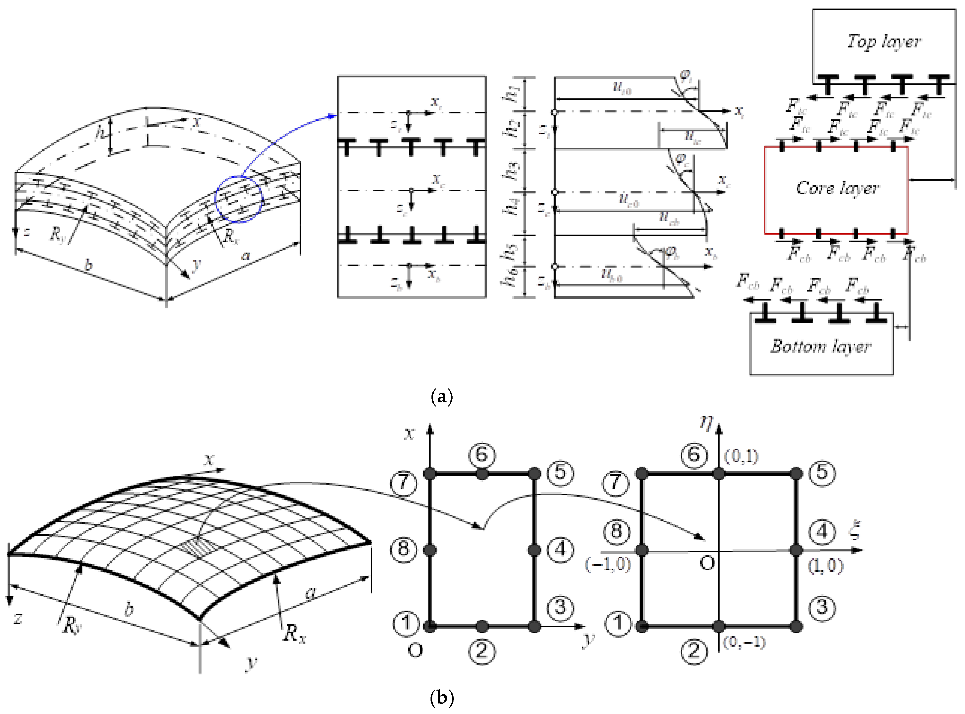
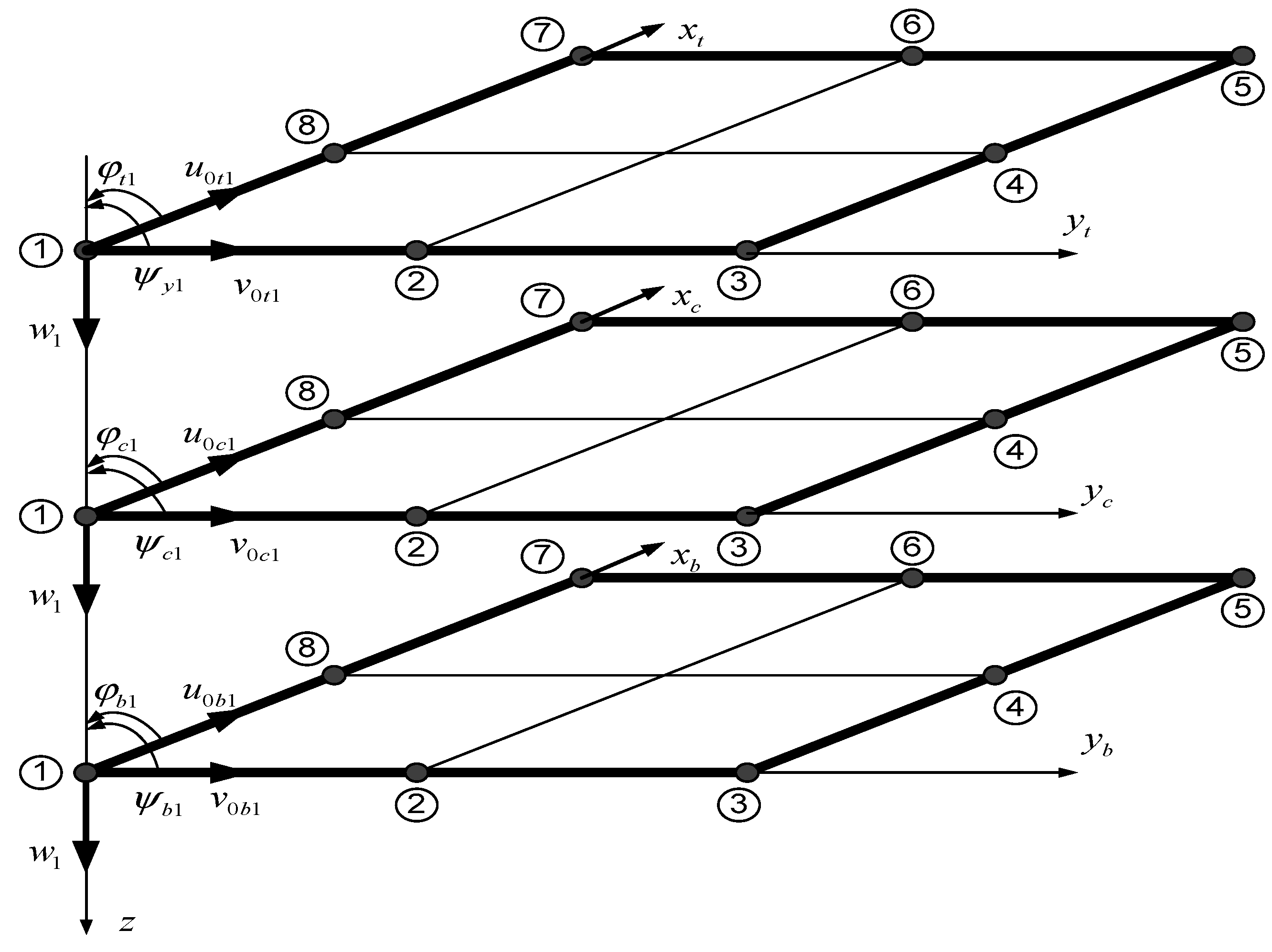
2.1. Equation of Motion of the Shell Element

Consider a three-layer composite shell with shear connectors as shown in Figure 1.

The composite shell consists of three layers, including the top layer (t), the bottom layer (b) and the middle layer (c); these layers are connected with one another by shear connectors, and they can be made of the same materials or different materials. These three layers can slide relatively with one another at the contact surfaces, and there is no delamination phenomenon at all. All three layers of the shell are set in the local coordinates Oxyt, Oxyc, and Oxyb, respectively. The total thickness of the shell is divided into six small part h₁, h₂, h₃, h₄, h₅, h₆ as shown in Figure 1; u_t0, u_c0, and u_b0 represent displacements in x direction; v_b0 represents the displacement in y direction at the neutral surface of each layer.

According to Mindlin plate theory, displacements u, v, w at a point (x_k, y_k, z_k) of layer k are expressed as follows:

$$\{\begin{array}{l}{u}_k=u_{k0}(x_k,y_k)+z_k{\phi }_k(x_k,y_k)\\ v_k=v_{k0}(x_k,y_k)+z_k{\psi }_k(x_k,y_k)\\ w_k=w(x_k,y_k)\end{array}\left(k=t,c,b\right)$$

(1)

where ${\phi }_k$ and ${\psi }_k$ are the transverse normal rotations of the x_k and y_k directions.

The relative movements among the contact surfaces are defined by the following equations

For the layer t and layer c we have

$$\{\begin{array}{l}{u}_{tc}=u_t(x_t,y_t,h_2)-u_c(x_c,y_c,-h_3)\\ v_{tc}=v_t(x_t,y_t,h_2)-v_c(x_c,y_c,-h_3)\end{array}$$

(2)

And for layer c and layer b we have:

$$\{\begin{array}{l}{u}_{cb}=u_c(x_c,y_c,h_4)-u_b(x_b,y_b,-h_5)\\ v_{cb}=v_c(x_c,y_c,h_4)-v_b(x_b,y_b,-h_5)\end{array}$$

(3)

Note that at the contact surfaces, we have:

$$\{\begin{array}{l}{z}_t=h_2;z_c=-h_3\\ z_c=h_4;z_b=-h_5\end{array}$$

(4)

with $h_4=h_3=\frac{h_c}{2}$.

From Equations (1)–(4), we get:

$$\{\begin{array}{c}{u}_{tc}=u_{t0}-u_{c0}+h_2{\phi }_t+h_3{\phi }_c\\ v_{tc}=v_{t0}-v_{c0}+h_2{\psi }_t+h_3{\psi }_c\end{array}$$

(5)

$$\{\begin{array}{c}{u}_{cb}=u_{c0}-u_{b0}+h_4{\phi }_c+h_5{\phi }_b\\ v_{cb}=v_{c0}-v_{b0}+h_4{\psi }_c+h_5{\psi }_b\end{array}$$

(6)

The relation between strain and displacement of each layer is expressed as follows

For the layer k, we have:

$$\begin{array}{l}{\epsilon }_{kx}=\frac{\partial u_k}{\partial x}=\frac{\partial u_{k0}}{\partial x}+\frac{w_0}{R_x}+z_k\frac{\partial {\phi }_k}{\partial x};\\ {\epsilon }_{ky}=\frac{\partial v_k}{\partial y}=\frac{\partial v_{k0}}{\partial y}+\frac{w_0}{R_y}+z_k\frac{\partial {\psi }_k}{\partial y};\\ {\gamma }_{kxy}=\frac{\partial v_k}{\partial x}+\frac{\partial u_k}{\partial y}=\frac{\partial u_{k0}}{\partial y}+\frac{\partial v_{k0}}{\partial x}+\frac{2w_0}{R_{xy}}+z_k\left(\frac{\partial {\phi }_k}{\partial y}+\frac{\partial {\psi }_k}{\partial x}+\frac{1}{2}(\frac{1}{R_y}-\frac{1}{R_x})\left(\frac{\partial v_{k0}}{\partial x}-\frac{\partial u_{k0}}{\partial y}\right)\right);\\ {\gamma }_{kxz}=\frac{\partial w_0}{\partial x}+\frac{\partial u_k}{\partial z_k}=\frac{\partial w_0}{\partial x}+{\phi }_k-\frac{u_{k0}}{R_x}-\frac{v_{k0}}{R_{xy}};\\ {\gamma }_{kyz}=\frac{\partial w_0}{\partial y}+\frac{\partial v_k}{\partial z_k}=\frac{\partial w_0}{\partial y}+{\psi }_k-\frac{u_{k0}}{R_{xy}}-\frac{v_{k0}}{R_y};\end{array}$$

(7)

We can rewrite in a matrix form as follow

$${\epsilon }_k=\left\{\begin{array}{c}{\epsilon }_{kx}\\ {\epsilon }_{ky}\\ {\gamma }_{kxy}\end{array}\right\}={\epsilon }_k^0+z_k{\kappa }_k; {\gamma }_k=\left\{\begin{array}{c}{\gamma }_{kyz}\\ {\gamma }_{kzx}\end{array}\right\}$$

(8)

in which

$$\begin{array}{l}{\epsilon }_k^0=\left\{\begin{array}{c}{\epsilon }_{kx}^0\\ {\epsilon }_{ky}^0\\ {\gamma }_{kxy}^0\end{array}\right\}=\left\{\begin{array}{c}\frac{\partial u_{k0}}{\partial x}+\frac{w_0}{R_x}\\ \frac{\partial v_{k0}}{\partial y}+\frac{w_0}{R_y}\\ \left(\frac{\partial u_{k0}}{\partial y}+\frac{\partial v_{k0}}{\partial x}\right)+\frac{2w_0}{R_{xy}}\end{array}\right\};{\kappa }_k=\left\{\begin{array}{l}{\kappa }_{kx}^{}\\ {\kappa }_{ky}^{}\\ {\kappa }_{kxy}^{}\end{array}\right\}=\left\{\begin{array}{c}\frac{\partial {\phi }_k}{\partial x}\\ \frac{\partial {\psi }_k}{\partial y}\\ \frac{\partial {\phi }_k}{\partial y}+\frac{\partial {\psi }_k}{\partial x}+\frac{1}{2}(\frac{1}{R_y}-\frac{1}{R_x})\left(\frac{\partial v_{k0}}{\partial x}-\frac{\partial u_{k0}}{\partial y}\right)\end{array}\right\}\\ {\gamma }_k=\left\{\begin{array}{l}{\gamma }_{kxz}^{}\\ {\gamma }_{kyz}^{}\end{array}\right\}=\left\{\begin{array}{l}-\frac{u_{k0}}{R_x}-\frac{v_{k0}}{R_{xy}}+\frac{\partial w_0}{\partial x}+{\phi }_k\\ -\frac{u_{k0}}{R_{xy}}-\frac{v_{k0}}{R_y}+\frac{\partial w_0}{\partial y}+{\psi }_k\end{array}\right\}\end{array}$$

(9)

The relation between stress and strain of layer k is expressed as followIs necessary bild?

$${\sigma }_k=D_k{\epsilon }_k; {\tau }_k=\frac{5}{6}{G}_k{\gamma }_k$$

(10)

in which $D_k, G_k$ are the bending rigidity and shear rigidity of layer k, respectively, and ${\nu }_k$ is the Poisson ratio of layer k.

$$D_k=\frac{E_k}{1-v^2}\left[\begin{array}{ccc}1& {\nu }_k& 0\\ {\nu }_k& 1& 0\\ 0& 0& (1-{\nu }_k)/2\end{array}\right]; G_k=\frac{E_k^{}}{2(1+{\nu }_k)}\left[\begin{array}{cc}1& 0\\ 0& 1\end{array}\right]$$

(11)

In this work, the thickness of the shell is thin or medium ($h=\frac{a}{100}÷\frac{a}{10}$, a is short edge), we employ the 8-node isoparametric element, each node has 13 degrees of freedom, three layers have the same displacement in the z-direction (Figure 2), the degree of freedom of node i is $q_e^i$ and the total degree of freedom of the shell element $q_e$ is defined as follow.

$$q_e^i={\left\{\begin{array}{cccccccccccc}{u}_{t0i}& v_{t0i}& {\phi }_{ti}& {\psi }_{ti}& u_{c0i}& v_{c0i}& {\phi }_{ci}& {\psi }_{ci}& u_{b0i}& v_{b0i}& {\phi }_{bi}& {\psi }_{bi}\end{array}w\right\}}^{\mathrm{T}}; i=1÷8.$$

(12)

$$q_e={\left\{\begin{array}{cccc}{q}_e^1& q_e^2& q_e^3& q_e^4\begin{array}{cccc}{q}_e^5& q_e^6& q_e^7& q_e^8\end{array}\end{array}\right\}}^{\mathrm{T}}$$

(13)

$$\begin{array}{l}{u}_{k0}={\displaystyle \sum _{i=1}^8{N}_i\left(\xi ,\eta \right)}{u}_{k0i}; v_{k0}={\displaystyle \sum _{i=1}^8{N}_i\left(\xi ,\eta \right)}{v}_{k0i}\\ {\phi }_k={\displaystyle \sum _{i=1}^8{N}_i\left(\xi ,\eta \right)}{\phi }_{ki}; {\psi }_k={\displaystyle \sum _{i=1}^8{N}_i\left(\xi ,\eta \right)}{\psi }_{ki}; w={\displaystyle \sum _{i=1}^8{N}_i}\left(\zeta ,\eta \right)w_i\end{array}(k=t,c,b)$$

(14)

in which N_i (i = 1 ÷ 8) can be defined as in [28].

By substituting in the expression for verifying displacement of element we have:

$$\{\begin{array}{l}{\epsilon }_k=\left(B_k^0+z_k{B}_k^1\right)q_e\\ {\gamma }_k=S_k{q}_e\end{array} (k=t,c,b)$$

(15)

in which $B_k^0; B_k^1; S_k$ are defined as follows

$$\begin{array}{l}{B}_k^0=\left[\begin{array}{cccc}{B}_{k1}^0& B_{k2}^0& B_{k3}^0& B_{k4}^0\begin{array}{cccc}{B}_{k5}^0& B_{k6}^0& B_{k7}^0& B_{k8}^0\end{array}\end{array}\right];\\ B_k^1=\left[\begin{array}{cccc}{B}_{k1}^1& B_{k2}^1& B_{k3}^1& B_{k4}^1\begin{array}{cccc}{B}_{k5}^1& B_{k6}^1& B_{k7}^1& B_{k8}^1\end{array}\end{array}\right];\\ S_k=\left[\begin{array}{cccc}{S}_{k1}& S_{k2}& S_{k3}& S_{k4}\begin{array}{cccc}{S}_{k5}& S_{k6}& S_{k7}& S_{k8}\end{array}\end{array}\right];\end{array}$$

(16)

where $B_{ki}^0$, $B_{ki}^1$ and $S_{ki}^{}$ can be found in Appendix A

The elastic force of connector stub per unit length is defined by the following equations.

For layer t and c we have:

$$F_e^{tc}={\left\{\begin{array}{l}{F}_{eu}\\ F_{ev}\end{array}\right\}}_{ct}=k_{tc}\left[\begin{array}{cc}1& 0\\ 0& 1\end{array}\right]\left\{\begin{array}{l}{u}_{tc}\\ v_{tc}\end{array}\right\}=K_e^{tc}{q}_e^{tc}$$

(17)

With

$$q_e^{tc}=\left\{\begin{array}{c}{u}_{tc}\\ v_{tc}\end{array}\right\}=\left[\begin{array}{c}{u}_{t0}+h_2{\phi }_t-u_{c0}+h_3{\phi }_c\\ v_{t0}+h_2{\psi }_t-v_{c0}+h_3{\psi }_c\end{array}\right]=N_{tc}{q}_e={\displaystyle \sum _{i=1}^8{\left(N_{tc}\right)}_i{q}_e^i}$$

(18)

in which

$${\left(N_{tc}\right)}_i=\left[\begin{array}{ccccccccc}{N}_i& 0& h_2{N}_i& 0& -N_i& 0& h_3{N}_i& 0& 0\hspace{1em}0\hspace{1em}0\hspace{1em}0\hspace{1em}0\\ 0& N_i& 0& h_2{N}_i& 0& -N_i& 0& h_3{N}_i& 0\hspace{1em}0\hspace{1em}0\hspace{1em}0\hspace{1em}0\end{array}\right]$$

(19)

For layer c and b we have

$$F_e^{cb}={\left\{\begin{array}{l}{F}_{eu}\\ F_{ev}\end{array}\right\}}_{cb}=k_{cb}\left[\begin{array}{cc}1& 0\\ 0& 1\end{array}\right]\left\{\begin{array}{l}{u}_{cb}\\ v_{cb}\end{array}\right\}=K_e^{cb}{q}_e^{{}_{cb}}$$

(20)

with

$$q_e^{{}_{cb}}=\left\{\begin{array}{c}{u}_{cb}\\ v_{cb}\end{array}\right\}=\left[\begin{array}{c}{u}_{c0}+h_4{\phi }_c-u_{b0}+h_5{\phi }_b\\ v_{c0}+h_4{\psi }_c-v_{b0}+h_5{\psi }_b\end{array}\right]=N_{cb}{q}_e={\displaystyle \sum _{i=1}^8{\left(N_{cb}\right)}_i{q}_e^i}$$

(21)

in which

$${\left(N_{cb}\right)}_i=\left[\begin{array}{ccccccccc}0\hspace{1em}0\hspace{1em}0\hspace{1em}0\hspace{1em}{N}_i& 0& h_4{N}_i& 0& -N_i& 0& h_5{N}_i& 0& 0\\ 0\hspace{1em}0\hspace{1em}0\hspace{1em}0\hspace{1em}0& N_i& 0& h_4{N}_i& 0& -N_i& 0& h_5{N}_i& 0\end{array}\right]$$

(22)

Here, $k_{tc}$ and $k_{cb}$ are the shear resistance coefficients of the connector stub per unit length.

To obtain the dynamic equation we employ the weak form for each element, we get:

$$\begin{array}{l}{\displaystyle \sum _{k=t,c,b}{\displaystyle \underset{V_k}{\int }\delta {\dot{q}}_k^{\mathrm{T}}{\rho }_k{\dot{q}}_{k}d{V}_k}}+{\displaystyle \sum _{k=t,c,b}{\displaystyle \underset{V_k}{\int }\delta {\epsilon }_k^{\mathrm{T}}}}{\sigma }_k^{}d{V}_k+\frac{5}{6}{\displaystyle \sum _{k=t,c,b}{\displaystyle \underset{V_k}{\int }\delta {\gamma }_k^{\mathrm{T}}}}{\tau }_{k}d{V}_k+{\displaystyle \sum _{k=tc,cb}{\displaystyle \underset{A_k}{\int }\delta {\left(q_e^k\right)}_{}^{\mathrm{T}}}}{F}_e^{k}d{A}_k\\ -\delta q_e^{\mathrm{T}}{\displaystyle \underset{A_t}{\int }{N}_{\mathrm{w}}}p(t)d{A}_t=0\end{array}$$

(23)

By substituting Equations (1), (15), (17), and (20) into Equation (23), we obtain the dynamic equation of the shell element as follows:

$$M_e^{}{\ddot{q}}_e+K_e^{}{q}_e=F_e(t)$$

(24)

with

$$\begin{array}{l}{K}_{e\left(104\mathrm{x}104\right)}^{}={\displaystyle \sum _{k=c,s,a}{\displaystyle \underset{A_k}{\int }{\left(B_k^0\right)}^{\mathrm{T}}}}{D}_{k0}{B}_k^{0}d{A}_k+{\displaystyle \sum _{k=c,s,a}{\displaystyle \underset{A_k}{\int }{\left(B_k^0\right)}^{\mathrm{T}}{D}_{k1}{B}_k^{1}d{A}_k+}}\\ +{\displaystyle \sum _{k=t,c,b}{\displaystyle \underset{A_k}{\int }{\left(B_k^1\right)}^{\mathrm{T}}{D}_{k1}{B}_k^{0}d{A}_k+{\displaystyle \sum _{k=t,c,b}{\displaystyle \underset{A_k}{\int }{\left(B_k^1\right)}^{\mathrm{T}}{D}_{k2}{B}_k^{1}d{A}_k}}}}+\frac{5}{6}{\displaystyle \sum _{k=t,c,b}{\displaystyle \underset{A_k}{\int }{S}_k^T{G}_k{S}_k^{}d{A}_k}}\\ +{\displaystyle \underset{A_{tc}}{\int }{N}_{tc}^{\mathrm{T}}}{K}_{tc}^e{N}_{tc}d{A}_{tc}+{\displaystyle \underset{A_{cb}}{\int }{N}_{cb}^{\mathrm{T}}}{K}_{cb}^e{N}_{cb}d{A}_{cb}\end{array}$$

(25)

in which

$$\left(D_{k0}; D_{k1}; D_{k2}\right)={\displaystyle \underset{-h_k/2}{\overset{h_k/2}{\int }}\left(1; z_k; z_k^2\right)D_k} d{z}_k;\hspace{1em}{H}_k={\displaystyle \underset{-h_k/2}{\overset{h_k/2}{\int }}{G}_k} d{z}_k (k=t,c,b)$$

(26)

$$M_{e\left(104\mathrm{x}104\right)}^{}={\displaystyle \sum _{k=t,c,b}{\displaystyle \underset{A_k}{\int }{\displaystyle \underset{-h_k/2}{\overset{h_k/2}{\int }}{L}_k^{\mathrm{T}}{\rho }_k{L}_{k}d{z}_{k}d{A}_k}}}$$

(27)

where $L_k$ can be seen in Appendix B

$$F_e{(t)}_{\left(104\mathrm{x}1\right)}={\displaystyle \underset{A_t}{\int }p(t)N_{\mathrm{w}}^{\mathrm{T}}}d{A}_t$$

(28)

in which

$$N_w=\left[\begin{array}{cccc}{N}_{\mathrm{w}1}& N_{\mathrm{w}2}& N_{\mathrm{w}3}& N_{\mathrm{w}4}\begin{array}{cccc}{N}_{\mathrm{w}5}& N_{\mathrm{w}6}& N_{\mathrm{w}7}& N_{\mathrm{w}8}\end{array}\end{array}\right]$$

(29)

with

$$N_{\mathrm{w}}{}_j=\left[\begin{array}{ccccccccc}0& 0& 0& 0& 0& 0& 0& 0\hspace{1em}0\hspace{1em}0\hspace{1em}0\hspace{1em}0& N_j\end{array}\right]$$

(30)

In the case of taking into account the structural damping, we have the force vibration equation of the shell element as follows:

$$M_e^{}{\ddot{q}}_e+C_e^{}{\dot{q}}_e+K_e^{}{q}_e=F_e(t)$$

(31)

in which $C_e^{}=\alpha M_e^{}+\beta K_e^{}$ and $\alpha , \beta$ are Rayleigh drag coefficients defined in [30,31].

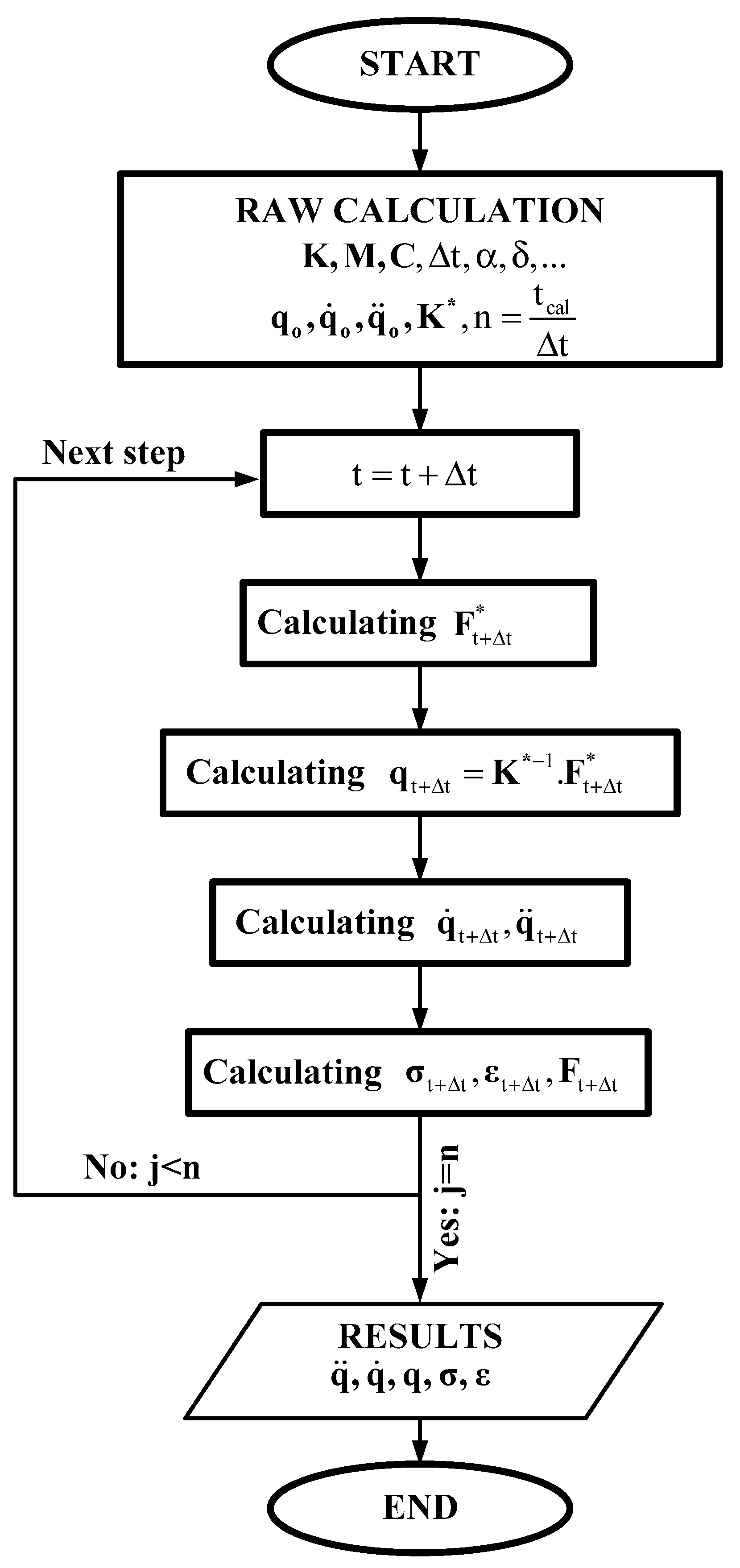
2.2. The Differential Equation of Vibration

From the differential equation of vibration of the shell element (Equation (31)), we obtain the differential equation of forced vibration of three-layer composite shell as follows:

$$M\ddot{q}+Cq+Kq=F(t)$$

(32)

in which $M$, $C$, $K$, $F(t)$ are the global mass matrix, the global structural damping matrix, the global stiffness matrix and the global load matrix, respectively. These matrices and vectors are assembled from the element matrices and vectors, correspondingly. They are linear differential equations, which have the right-hand side depending on time. In order to solve these equations, we use the Newmark-beta method [31]. The program is coded in the MATLAB (MathWorks, Natick, MA, USA) environment with the following algorithm flowchart of Newmark as shown Figure 3.

For the free vibration analysis, the natural frequencies can be obtained by solving the equation:

$$M\ddot{q}+Kq=0$$

(33)

or in another form:

$$\left(K-{\omega }^{2}M\right)q=0$$

(34)

where $\omega$ is the natural frequency.

Flowchart of Newmark-beta method [31]

Step 1: Determine the first conditions:

$$q(0)=q_0;\dot{q}(0)={\dot{q}}_0$$

(35)

From the first conditions, we obtain:

$${\ddot{q}}_0=M_0^{-1}\left(F_0-K_0{q}_0-C_0{\dot{q}}_0\right)$$

(36)

Step 2: By approximating ${\ddot{q}}_{t+\Delta t},{\dot{q}}_{t+\Delta t}$ by $q_{t+\Delta t}$, we have

$$\begin{array}{l}{\ddot{q}}_{t+\Delta t}=a_0\left(q_{t+\Delta t}-q_t\right)-a_2{\dot{q}}_t-a_3{\ddot{q}}_t\\ {\dot{q}}_{t+\Delta t}={\dot{q}}_t+a_6{\ddot{q}}_t+a_7{\ddot{q}}_{t+\Delta t}\end{array}$$

(37)

where:

$$\begin{gathered} a_0=\frac{2}{\gamma \Delta t^2}; a_1=\frac{2\alpha }{\gamma \Delta t}; a_2=\frac{2}{\gamma \Delta t}; a_3=\frac{1}{\gamma }-1; a_4=\frac{2\alpha }{\gamma }-1; \\ {a}_5=\left(\frac{\alpha }{\gamma }-1\right)\Delta t; a_6=\left(1-\alpha \right)\Delta t; a_7=\alpha \Delta t. \end{gathered}$$

(38)

in which $\alpha , \gamma$ are defined by the assumption that the acceleration varies in each calculating step, the author selects the linear law for the varying of acceleration:

$$\ddot{q}\left(\tau \right)={\ddot{q}}_t+\frac{\tau }{\Delta t}\left({\ddot{q}}_{t+\Delta t}-{\ddot{q}}_t\right) \mathrm{with} t\le \tau \le t+\Delta t \mathrm{then} \alpha =\frac{1}{2};\gamma =\frac{1}{3}.$$

(39)

The condition to stabilize the roots:

$$\Delta t\le \frac{1}{\sqrt{2}{\varpi }_{\max }}\frac{1}{\sqrt{\alpha -\gamma }} \mathrm{or} \frac{\Delta t}{T_{\min }}\le \frac{1}{2\pi \sqrt{2}}\frac{1}{\sqrt{\alpha -\gamma }}$$

(40)

Step 3: Calculating the stiffness matrix and the nodal force vector:

$$K^{\ast }=\overline{K}+a_0\overline{M}+a_1\overline{C}$$

(41)

$$F_{}^{\ast }={\overline{F}}_{t+\Delta t}+\overline{M}\left(a_0{q}_t+a_2{\dot{q}}_t+a_3{\ddot{q}}_t\right)+\overline{C}\left(a_1{q}_t+a_4{\dot{q}}_t+a_5{\ddot{q}}_t\right)$$

(42)

Step 4: Determining nodal displacement vector $q_{t+\Delta t}$:

$$K^{\ast }{}_{t+\Delta t}{q}_{t+\Delta t}=F^{\ast }{}_{t+\Delta t}$$

(43)

$$\Rightarrow q_{t+\Delta t}={\left(K^{\ast }{}_{t+\Delta t}\right)}^{-1}{F}^{\ast }{}_{t+\Delta t}$$

(44)

repeating the loop until the time runs out.

3. Numerical Results of Free Vibration Analysis of Three-Layer Composite Shells with Shear Connectors

3.1. Accuracy Studies

Consider a double-curved composite shell (0⁰/90⁰/0⁰) with geometrical parameters a = b, radii R_x = R_y = R, thickness h; physical parameters E₁ = 25E₂, G₂₃ = 0.2E₂, G₁₃ = G₁₂ = 0.5E₂, the Poisson’s ratio ${\nu }_{12}$ = 0.25, and the specific weight $\rho$. In this case, the shear coefficient of the stub has a very large value, and this time the three-layer composite shell becomes a normal composite shell without any relative movements. We examine the convergence of the algorithm with different meshes and the comparative results of the first non-dimensional free vibration $\overline{\omega }={\omega }_1\frac{a^2}{h}\sqrt{\frac{\rho }{E_2}}$ with Reddy [32] are shown in

Table 1. The first non-dimensional fundamental frequencies with different meshes.

a/h = 100		This Work					Reddy [32]
Meshes		4 × 4	6 × 6	8 × 8	10 × 10	12 × 12
R/a	1	126.430	126.135	126.145	126.145	126.145	125.99
	2	68.489	68.095	68.065	68.065	68.065	68.075
	3	47.432	47.316	47.369	47.369	47.369	47.265
	4	36.989	36.975	37.083	37.083	37.083	36.971
	5	31.188	30.908	31.030	31.030	31.030	30.993
	10	20.313	20.350	20.332	20.332	20.332	20.347
	1030	15.174	5.151	15.1457	15.1457	15.1457	15.183
a/h = 10		This Work					Reddy [32]
Meshes		4 × 4	6 × 6	8 × 8	10 × 10	12 × 12
R/a	1	16.3576	16.3272	16.3226	16.3226	16.3226	16.115
	2	12.9939	12.9811	12.978	12.978	12.978	13.382
	3	12.1582	12.1500	12.1488	12.1488	12.1488	12.731
	4	11.8418	11.8354	11.8343	11.8343	11.8343	12.487
	5	11.6905	11.6851	11.6843	11.6843	11.6843	12.372
	10	11.4843	11.4799	11.4791	11.4791	11.4791	12.215
	1030	11.4141	11.4102	11.4095	11.4095	11.4095	12.165

.

From Table 1 we can see clearly that, in comparison between this work and the analytical method [32], we have good agreement, demonstrating that our proposed theory and program are verified for the free vibration problem and convergence is guaranteed with 8 × 8 meshes.

3.2. Effects of Some Parameters on Free Vibration of the Shell

We now consider a three-layer composite shell with geometrical parameters: length a is constant, width b, radii R_x = R_y = R, the total thickness h, the thickness of the middle layer h_c, the thicknesses of the other layers h_t = h_b (h₁ = h₂ = h_t/2, h₃ = h₄ = h_c/2, h₅ = h₆ = h_b/2); physical parameters: the elastic modulus E_c = 70 GPa, E_t = E_b = 200 GPa, the Poisson’s ratio ${\nu }_t={\nu }_c={\nu }_b=0.3$, the specific weight ${\rho }_c=2300$ kg/m³,${\rho }_t={\rho }_b=7800$ kg/m³, the shear coefficient of the shear connector k_tc = k_c = k_s, and the shell structure is fully supported. We conduct an investigation into the first non-dimensional free vibration of the shell with non-dimensional frequencies as defined by:

$$\overline{\omega }={\omega }_1\frac{a^2}{h_0}\sqrt{\frac{{\rho }_t}{E_t}}\hspace{1em}\hspace{1em}\mathrm{with} h_0=\frac{a}{50}$$

(45)

3.2.1. Effect of Thickness h

Firstly, to examine the effect of length-to-high ratio a/h, a is fixed, we consider three cases with a/h = 75, 60, 50, 25, 10 (respectively). In each case, the radius-to-length ratio R/a changes from 1 to 10 as we can see in

Table 2. Effect of thickness h on non-dimensional fundamental frequencies.

R/a	a/h = 75	a/h = 60	a/h = 50	a/h = 25	a/h = 10
1	48.9232	48.9329	48.9447	49.0591	49.8350
2	25.2821	25.3022	25.3267	25.5643	27.1440
3	16.9857	17.0161	17.0531	17.4099	19.6929
4	12.7982	12.8388	12.8881	13.3594	16.2390
5	10.2817	10.3324	10.3938	10.9744	14.3496
6	8.6065	8.6671	8.7403	9.4243	13.2070
7	7.4135	7.4838	7.5686	8.3498	12.4663
8	6.5225	6.6024	6.6983	7.5705	11.9605
9	5.8331	5.9222	6.0291	6.9856	11.6008
10	5.2847	5.3830	5.5004	6.5351	11.3363

, b = a, h_c/h_t = 2, and the shear coefficient of stub k_s = 50 MPa. The results are presented in Table 2.

Table 2 demonstrates that when the length-to-high ratio a/h decreases, that means the stiffness of the structure is enhanced, correspondingly with each case of the radius-to-length ratios R/a, the non-dimensional fundamental frequency increases.

3.2.2. Effect of the h_c/h_t Ratio (h_t = h_b)

Next, in order to study the effect of the h_c/h_t ratio, we consider five cases with h_c/h_t, respectively given values from 2, 4, 8, 20, 30, b = a (a is fixed), the total thickness h = a/50, and the shear coefficient of the stub k_s = 50 MPa. The numerical results are shown in

Table 3. Effect of h_c/h_t ratio on non-dimensional fundamental frequencies.

R/a	hc/ht = 2	hc/ht = 4	hc/ht = 8	hc/ht = 20	hc/ht = 30
1	48.9447	49.6002	50.3956	51.3623	51.6856
2	25.3267	25.7143	26.2246	26.8744	27.0959
3	17.0531	17.3679	17.8202	18.4208	18.6285
4	12.8881	13.1816	13.6348	14.2529	14.4682
5	10.3938	10.6864	11.1625	11.8208	12.0502
6	8.7403	9.0417	9.5499	10.2558	10.5011
7	7.5686	7.8839	8.4277	9.1822	9.4432
8	6.6983	7.0301	7.6105	8.4117	8.6871
9	2.6219	6.3787	6.9948	7.8393	8.1278
10	2.5746	5.8683	6.5186	7.4026	7.7027

.

Table 3 gives us a discussion that when increasing h_c/h_t ratio, and for h is constant, that means the thickness of the middle layer increases, correspondingly each case of R/a ratios, the non-dimensional fundamental frequency increases. This shows that when the thickness of the shell is constant, h_c/h_t increases, thus, the non-dimensional fundamental frequency increases.

3.2.3. Effect of the Length-to-Width Ratio a/b

In this small section, we continually evaluate the effect of the length-to-width ratio a/b (a is fixed), and we meditate three cases by letting a/b = 0.5, 0.75, 1, 1.75, and 2, respectively. The total thickness of the shell h = a/50, h_c/h_t = 2, the radius-to-length R/a also varies from 1 to 10, as we can see in

Table 4. Effect of length-to-width ratio a/b on non-dimensional fundamental frequencies.

R/a	a/b = 0.5	a/b = 0.75	a/b = 1	a/b = 1.5	a/b = 2
1	47.6987	48.3535	48.9447	49.8156	50.4172
2	25.1170	25.2201	25.3267	25.5626	25.9090
3	16.9310	16.9833	17.0531	17.2818	17.7252
4	12.7690	12.8155	12.8881	13.1627	13.7259
5	10.2602	10.3104	10.3938	10.7236	11.4034
6	8.5872	8.6438	8.7403	9.1263	9.9146
7	7.3943	7.4584	7.5686	8.0095	8.8965
8	6.5025	6.5743	6.6983	7.1919	8.1678
9	5.8117	5.8914	6.0291	6.5726	7.6279
10	5.2618	5.3494	5.5004	6.0909	7.2169

, and the shear coefficient of stub k_s = 50 MPa. The numerical results are tabulated in Table 4.

In Table 4 we can see obviously that, with each value of radius-to-length R/a, if the length-to-width a/b increases, the non-dimensional fundamental frequency also increases, correspondingly. This interesting point demonstrates that the stiffness of the structure is enhanced.

3.2.4. Effect of the Shear Coefficient of Stub k_s

Finally, in this section, to examine how the shear coefficient of the stub affects the non-dimensional fundamental frequencies of this structure, we consider three cases of shear coefficient as in

Table 5. Effect of shear coefficient of the stub k_s on non-dimensional fundamental frequencies.

R/a	$\frac{{\mathit{k}}_{\mathit{s}}}{{\mathit{E}}_{\mathit{c}}}=1.45\times {10}^{-5}$	$\frac{{\mathit{k}}_{\mathit{s}}}{{\mathit{E}}_{\mathit{c}}}=1.45\times {10}^{-2}$	$\frac{{\mathit{k}}_{\mathit{s}}}{{\mathit{E}}_{\mathit{c}}}=1.45\times {10}^0$	$\frac{{\mathit{k}}_{\mathit{s}}}{{\mathit{E}}_{\mathit{c}}}=1.45\times {10}^2$	$\frac{{\mathit{k}}_{\mathit{s}}}{{\mathit{E}}_{\mathit{c}}}=1.45\times {10}^5$
1	48.9437	48.9457	49.0792	49.3528	49.3628
2	25.3247	25.3288	25.6047	26.1739	26.1918
3	17.0500	17.0562	17.4689	18.3090	18.3350
4	12.8840	12.8922	13.4361	14.5187	14.5518
5	10.3887	10.3989	11.0674	12.3634	12.4024
6	8.7342	8.7463	9.5324	11.0130	11.0568
7	7.5615	7.5756	8.4716	10.1104	10.1582
8	6.6904	6.7062	7.7046	9.4781	9.5291
9	6.0202	6.0379	7.1307	9.0186	9.0722
10	5.4907	5.5100	6.6899	8.6749	8.7306

, and a = b, h = a/50, h_c/h_t = 2, E_c = 70 GPa is fixed. The numerical results are shown in this table.

In Table 5 we can see clearly that, with one value of radius-to-length R/a, when the shear coefficient of stub increases, the non-dimensional fundamental frequency of the structure get larger. This explains that the increasing of the shear coefficient removes the slip among layers, leading to an increase of the total stiffness of the shell structure.

4. Numerical Results of Forced Vibration Analysis of Three-Layer Composite Shells with Shear Connectors

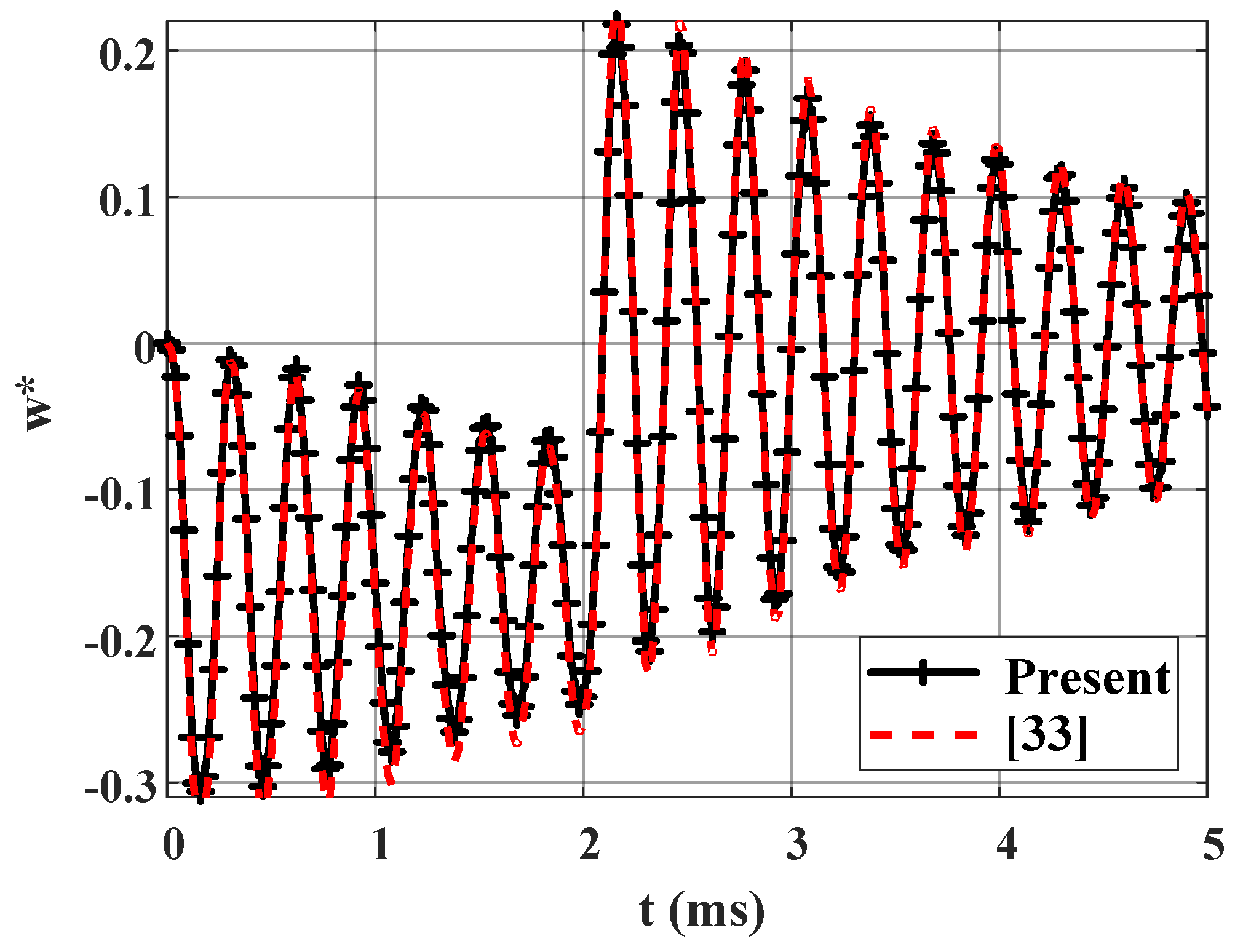
4.1. Accuracy Studies

Considerign that a fully-clamped square plate with parameters can be found in [33], a = b = 1m, h/a = 10. Material properties are the elastic modulus E = 30 GPa, the Poisson’s ratio ν = 0.3, ρ = 2800 kg/m³. The structure is subjected to distribution sudden load p₀ = 10⁴ Pa. The non-dimensional displacement is calculated by the formula $w^{\ast }=\frac{100E{h}^3}{12p_0{a}^4(1-{\nu }^2)}{w}_0$. By taking the shear coefficient and radii of the shell as very large, the comparative deflection of the centroid point of the plate between our work and [33] is shown in Figure 4, where the integral time is 5 ms, and the acting time of load is 2 ms.

We can see from Figure 4 that the deflection of the centroid point of the plate is compared to [33] is similar both shape and value. This proves that our program is verified.

4.2. Effect of Some Parameters on the Forced Vibration of the Shell

Now, to study effects of some parameters on forced vibration of shell, we consider a three-layer composite shell with geometrical parameters: length a =1 m, width b, thickness h, radii of the shell R_x = R_y = R, the thickness of middle layer h_c, the thickness of other layers h_t = h_b. Material properties are the elastic modulus E_c = 8 GPa, E_t = E_b = 12 GPa, the Poisson’s ratio ${\nu }_t={\nu }_c={\nu }_b=0.2$, the specific weight ${\rho }_c=700$ kg/m³, ${\rho }_t={\rho }_b=2300$ kg/m³, and the shear coefficient of stub k_tc = k_cb = k_s. The shell is fully clamped with the uniform load p(t) varying overtime acting perpendicularly on the shell surface.

$$p(t)=\Delta P_{\Phi }.F(t);\hspace{1em}F(t)=\{\begin{array}{l}1-\frac{t}{{\tau }_{hd}}\hspace{1em}\left(0\le t\le {\tau }_{hd}\right)\\ 0\hspace{1em}\hspace{1em}\mathrm{otherwise}\end{array}\hspace{1em}\mathrm{with}\hspace{1em}\{\begin{array}{l}\Delta P_{\Phi }={\mathrm{0.20679.10}}^6 \mathrm{N}/{\mathrm{m}}^2\\ {\tau }_{hd}=0.028 s\end{array}$$

(46)

The non-dimensional deflection and velocity of the centroid point over time are given as follows:

$$\begin{array}{l}{w}^{\ast }=\frac{100h_0{}^3{E}_t}{\Delta P_{\Phi }{a}^4}w\left(\frac{a}{2},\frac{b}{2}\right); v^{\ast }=\frac{T{h}_0{}^3{E}_t}{\Delta P_{\Phi }{a}^4}v\left(\frac{a}{2},\frac{b}{2}\right)\\ u_c^{\ast }=\frac{10h_0{}^3{E}_c}{Mg{a}^2(1-{\nu }_c^2)}{u}_c\left(\frac{a}{2},\frac{b}{2},-\frac{h_c}{2}\right);v_c^{\ast }=\frac{10h_0{}^3{E}_c}{Mg{a}^2(1-{\nu }_c^2)}{v}_c\left(\frac{a}{2},\frac{b}{2},-\frac{h_c}{2}\right)\mathrm{with} h_0=\frac{a}{50}; T=0.15(s)\end{array}$$

(47)

where $w\left(\frac{a}{2},\frac{b}{2}\right)$ and $v\left(\frac{a}{2},\frac{b}{2}\right)$ are the deflection and velocity of the centroid point of the shell.

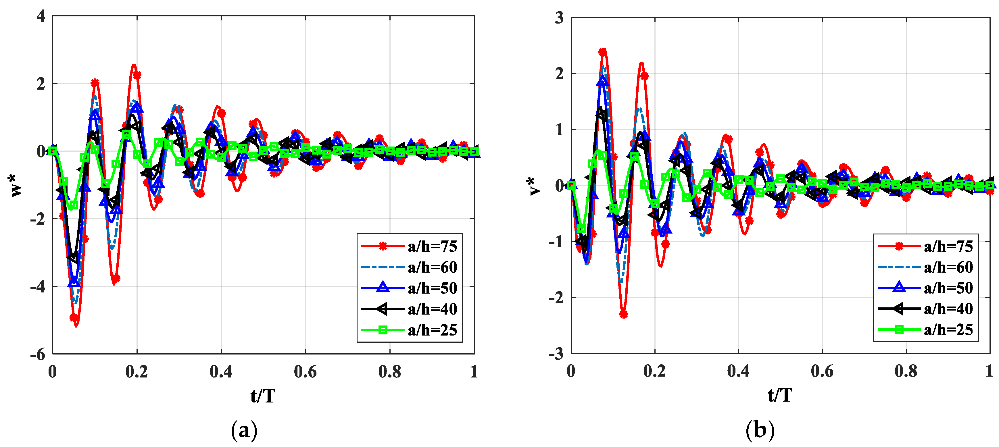
4.2.1. Effect of the Length-to-High Ratio a/h

In this first small section, we study the effect of the length-to-high ratio a/h. We consider a shell with geometrical parameters a = b (a is fixed), h_c/h_t = 2, R/a = 6, and a/h gets value 75, 60, 50, 40 and 25, respectively, the shear coefficient of stub k_s = 50 MPa. The non-dimensional deflection and velocity of the centroid point of the shell are presented in Figure 5 and the maximum value is shown in

Table 6. Effect of length-to-high ratio a/h the non-dimensional deflection and velocity of the centroid point.

Maximum Values	a/h = 75	a/h = 60	a/h = 50	a/h = 40	a/h = 25
${\mathrm{w}}_{\max }^{\ast }$	5.1866	4.5001	3.9020	3.1534	1.7250
${\mathrm{v}}_{\max }^{\ast }$	2.2997	1.7296	1.3653	1.1890	0.7686

.

From Figure 4 and Table 6 we can see that when reducing the value of a/h ratio, this means the thickness of the shell gets thicker, the non-dimensional deflection and velocity of the centroid point overtime decrease. This is a good agreement, the reason is when the thickness of the shell increases, the stiffness of the shell obviously becomes higher.

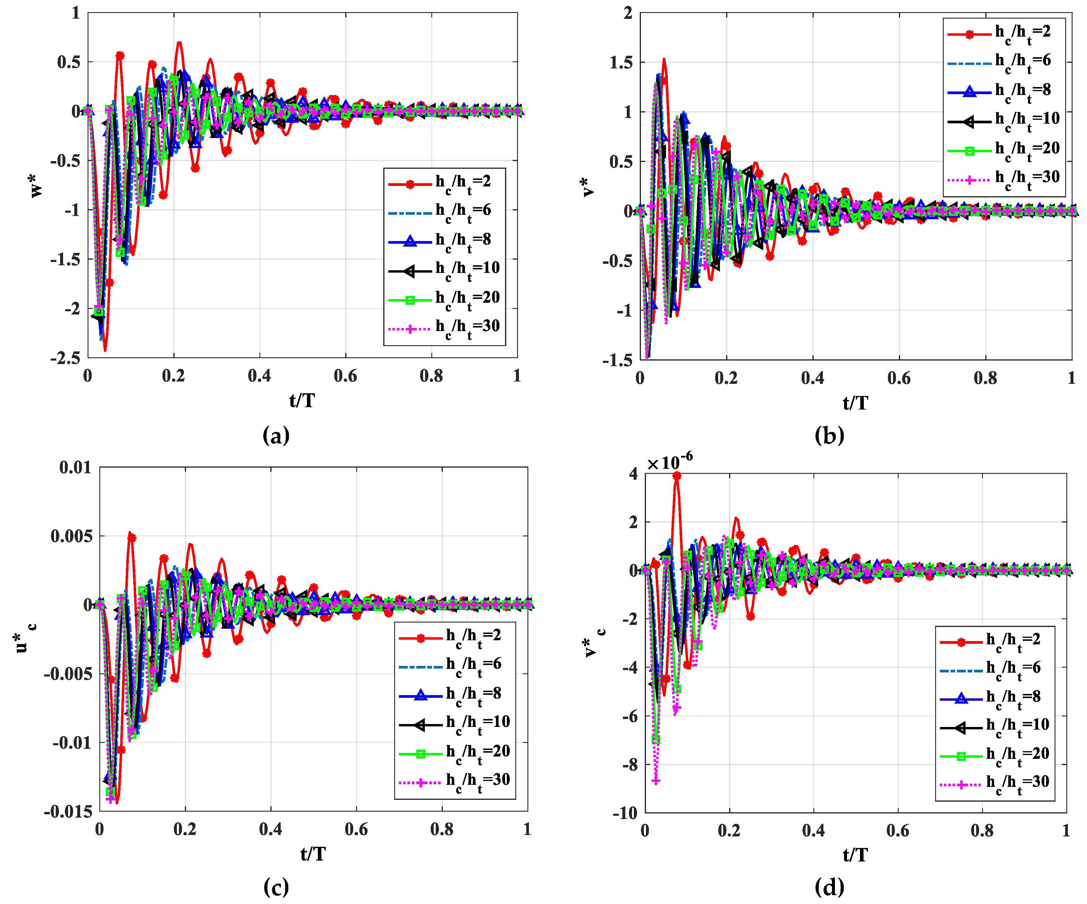
4.2.2. Effect of the h_c/h_t Ratio (h_t = h_b)

Next, to investigate the effect of h_c/h_t ratio, we dissect the shell with geometrical parameters a = b (a is fixed); h = a/50, the value of h_c/h_t ratio is given as 2, 6, 8, 10, 20, and 30, R/a = 6, and the shear coefficient of stub k_s = 50 (MPa). The non-dimensional deflection and velocity of the centroid point of the shell are shown in Figure 6, the maximum value is listed in

Table 7. Effect of h_c/h_t ratio on the non-dimensional deflection and velocity of the centroid point.

Maximum Values	hc/ht = 2	hc/ht = 6	hc/ht = 8	hc/ht = 10	hc/ht = 20	hc/ht = 30
${\mathrm{w}}_{\max }^{\ast }$	2.4284	2.3267	2.2499	2.1578	2.0313	1.9787
${\mathrm{u}}_c^{\ast \max }\times {10}^{-5}$	1.1921	1.8455	1.9861	1.990	2.1182	2.1605
$v_c^{\ast \max }\times {10}^{-6}$	5.1472	4.8345	5.0843	5.4432	6.9771	8.6697
${\mathrm{v}}_{\max }^{\ast }$	1.1221	1.4232	1.4658	1.4525	1.4479	1.4879

.

We can see in Figure 6 and Table 7 that when the h_c/h_t ratio increases (h is constant), the thickness of the middle layer increases in comparison to the other layers, and the non-dimensional deflection and velocity of the centroid point overtime decreases quickly in a range from 2–20. In a range from 20–30 the non-dimensional deflection and velocity of the centroid point overtime are almost not changed. The reason is explained that when the value of the h_c/h_t ratio increases, the structure can reduce the ability to oscillate, and the middle layer becomes “softer”, so that it imbues the vibration better than a homogeneous shell with same geometrical and physical parameters. For this particular problem, we should select the value of h_c/h_t ratio in a range from 20–30.

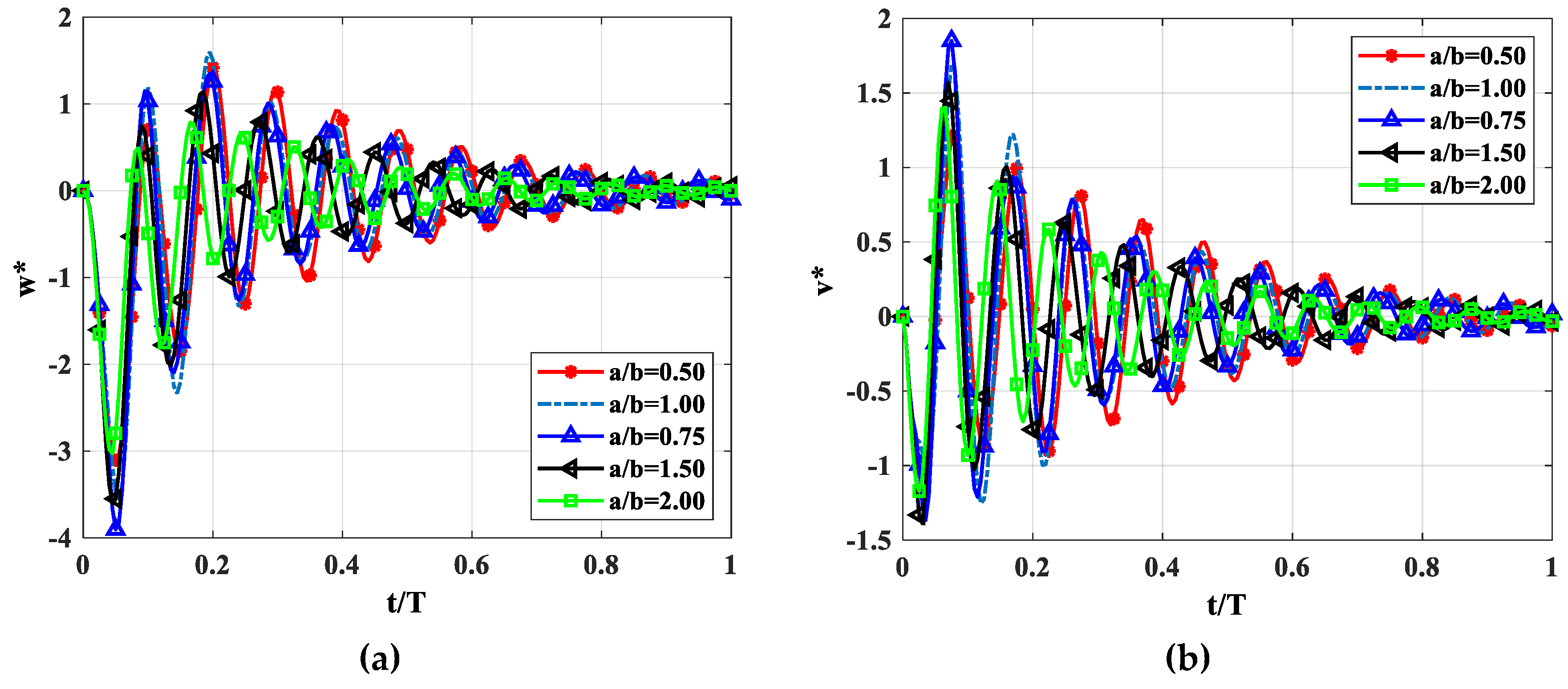
4.2.3. Effect of the Length-to-Width Ratio a/b

We examine the effect of length-to-width ratio a/b on the non-dimensional deflection and velocity of the centroid point of the shell with a is fixed, a/b gets from 0.5, 1, 1.5, 2. The geometrical parameters are h = a/50, h_c/h_t = 2, R/a = 6, and the shear coefficient of stub k_s = 50 MPa. The numerical results of non-dimensional deflection and velocity of the centroid point of the shell are shown in Figure 7, and the maximum value is listed in the following

Table 8. Effect of the length-to-width ratio a/b on the non-dimensional deflection and velocity of the centroid point.

Maximum Values	a/b = 0.5	a/b = 0.75	a/b = 1	a/b = 1.5	a/b = 2
${\mathrm{w}}_{\max }^{\ast }$	3.1051	3.5580	3.9020	3.6051	3.0260
${\mathrm{v}}_{\max }^{\ast }$	1.0248	1.2536	1.3653	1.3871	1.1701

.

Now we can see in Figure 7 and Table 8, when increasing the a/b ratio, the non-dimensional deflection and velocity of the centroid point overtime decrease. This demonstrates that the stiffness of the shell gets larger, especially when the a/b ratio equals 2. This can be understood obviously that as the shape of structure gets smaller, with the same boundary condition and other parameters, the structure will become stronger.

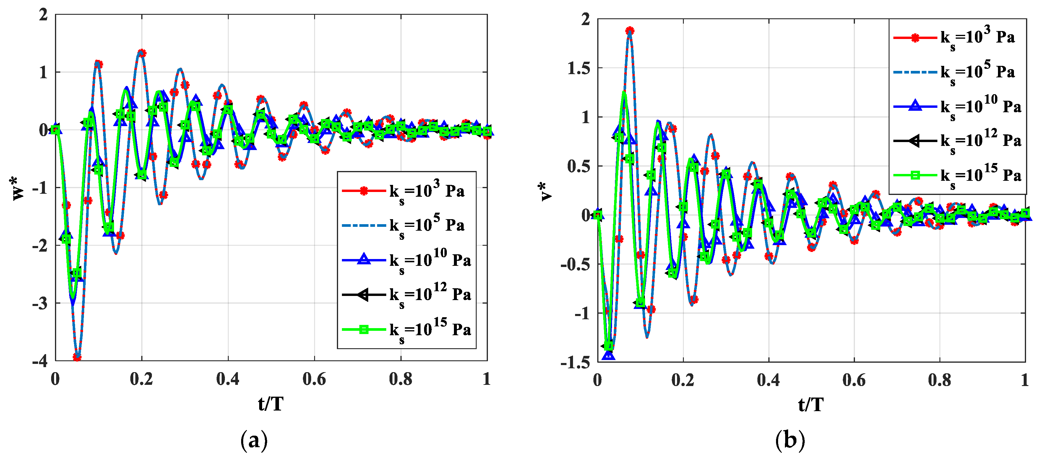
4.2.4. Effect of the Shear Coefficient of the Stub

Finally, we conduct a study on the effect of the shear coefficient of the stub on the non-dimensional deflection and velocity of the centroid point of the shell. We consider four cases with k_s = 10³, 10⁵, 10¹⁰, 10¹², and 10¹⁵ Pa. Geometrical parameters are a = b; h = a/50, h_c/h_t = 2, R/a = 6. The numerical results of non-dimensional deflection and velocity of the centroid point of the shell are plotted in Figure 8, the maximum value is shown in

Table 9. Effect of shear coefficient of stub on the non-dimensional deflection and velocity of the centroid point.

Maximum Values	${\mathit{k}}_{\mathit{s}}={10}^3\mathbf{Pa}$	${\mathit{k}}_{\mathit{s}}={10}^5\mathbf{Pa}$	${\mathit{k}}_{\mathit{s}}={10}^{10}\mathbf{Pa}$	${\mathit{k}}_{\mathit{s}}={10}^{12}\mathbf{Pa}$	${\mathit{k}}_{\mathit{s}}={10}^{15}\mathbf{Pa}$
${\mathrm{w}}_{\max }^{\ast }$	3.9352	3.9352	3.0341	2.9070	2.9059
${\mathrm{v}}_{\max }^{\ast }$	1.3658	1.3658	1.4354	1.3657	1.3662

.

In this last case, we can see in Figure 8 and Table 9 that when the shear coefficient of the stub increases, the non-dimensional deflection and velocity of the centroid point of the shell is reduced. It is easily understood that the enhancing of the stiffness of the stud makes the total structure get stronger, meaning the stiffness of the shell is increased, correspondingly.

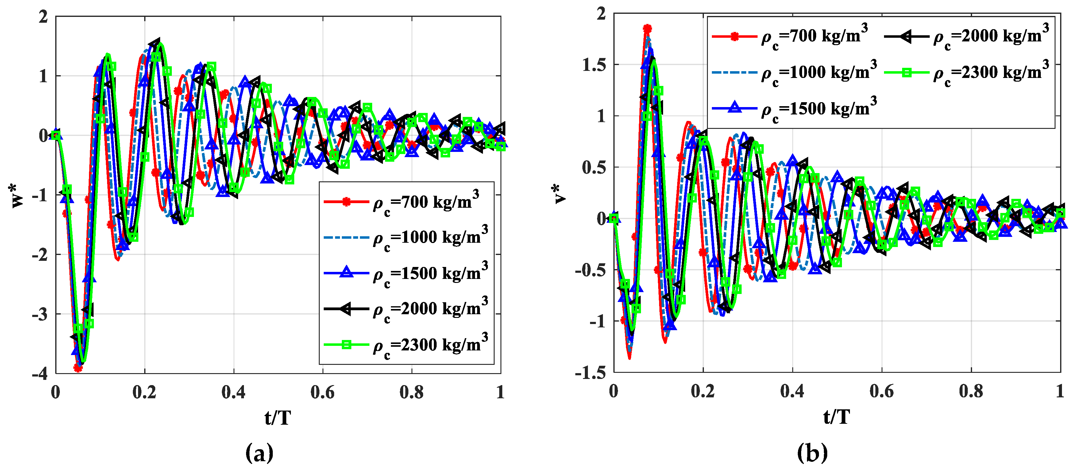
4.2.5. Influence of the Mass Density of the Core Layer

Let us consider a four-edge simply supported (SSSS) shell (b = a) with h_c = h/2, h_t = h_b = h/4. The shear modulus of the shear connector is k_s = 50 MPa. The mass densities of the three layers are ${\rho }_t={\rho }_b=2300$ kg/m³ and ${\rho }_c=700, 1000, 1500, 2000, 2300$ kg/m³. Nondimensional deflection and velocity of the shell center point are shown in Figure 9, maximum deflections and velocities of the shell center point are illustrated in

Table 10. Maximum deflections, velocities and stress of the shell center point versus time for different ${\rho }_c$.

Maximum Values	${\mathit{\rho }}_{\mathit{c}}= 700 (\mathbf{kg}/{\mathbf{m}}^3)$	${\mathit{\rho }}_{\mathit{c}}= 1000 (\mathbf{kg}/{\mathbf{m}}^3)$	${\mathit{\rho }}_{\mathit{c}}= 1500 (\mathbf{kg}/{\mathbf{m}}^3)$	${\mathit{\rho }}_{\mathit{c}}= 2000 (\mathbf{kg}/{\mathbf{m}}^3)$	${\mathit{\rho }}_{\mathit{c}}= 2300 (\mathbf{kg}/{\mathbf{m}}^3)$
${\mathrm{w}}_{\max }^{\ast }$	3.9020	3.8837	3.8403	3.8318	3.7942
${\mathrm{v}}_{\max }^{\ast }$	1.3653	1.2962	1.1985	1.1339	1.0871

. The mass ratio of the shell corresponding to the different values of ${\rho }_c$ compared to case ${\rho }_t={\rho }_c={\rho }_b=2300$ kg/m³ is shown in

Table 11. The mass ratio of the shell corresponding to the different values of ${\rho }_c$.

Mass Density of the Core Layer	${\mathit{\rho }}_{\mathit{c}}= 700$ (kg/m3)	${\mathit{\rho }}_{\mathit{c}}= 1000$ (kg/m3)	${\mathit{\rho }}_{\mathit{c}}= 1500$ (kg/m3)	${\mathit{\rho }}_{\mathit{c}}= 2000$ (kg/m3)	${\mathit{\rho }}_{\mathit{c}}= 2300$ (kg/m3)
The mass ratio ($100\frac{{\rho }_c+{\rho }_t}{2{\rho }_t}\%$)	65.21	71.73	82.60	93.44	100
Reduced mass ($\%$)	34.79	28.27	17.40	6.56	0

.

Comment: From the Figure 9 and Table 10 and Table 11, we obtain that when the mass density of the core-layer is increased from 700 to 2300 kg, deflection and velocity of the shell center point are almost not changed. Therefore, in order to reduce the mass of the shell, we can use the triple-layer shell with shear connectors, which the core layer has a smaller mass density than other layers. Specifically, corresponding to a difference of mass density of the core layer ${\rho }_c=700, 1000, 1500, 2000$ kg/m³, the mass of the shell decreases by 34.79, 28.27, 17.40, and 6.56%.

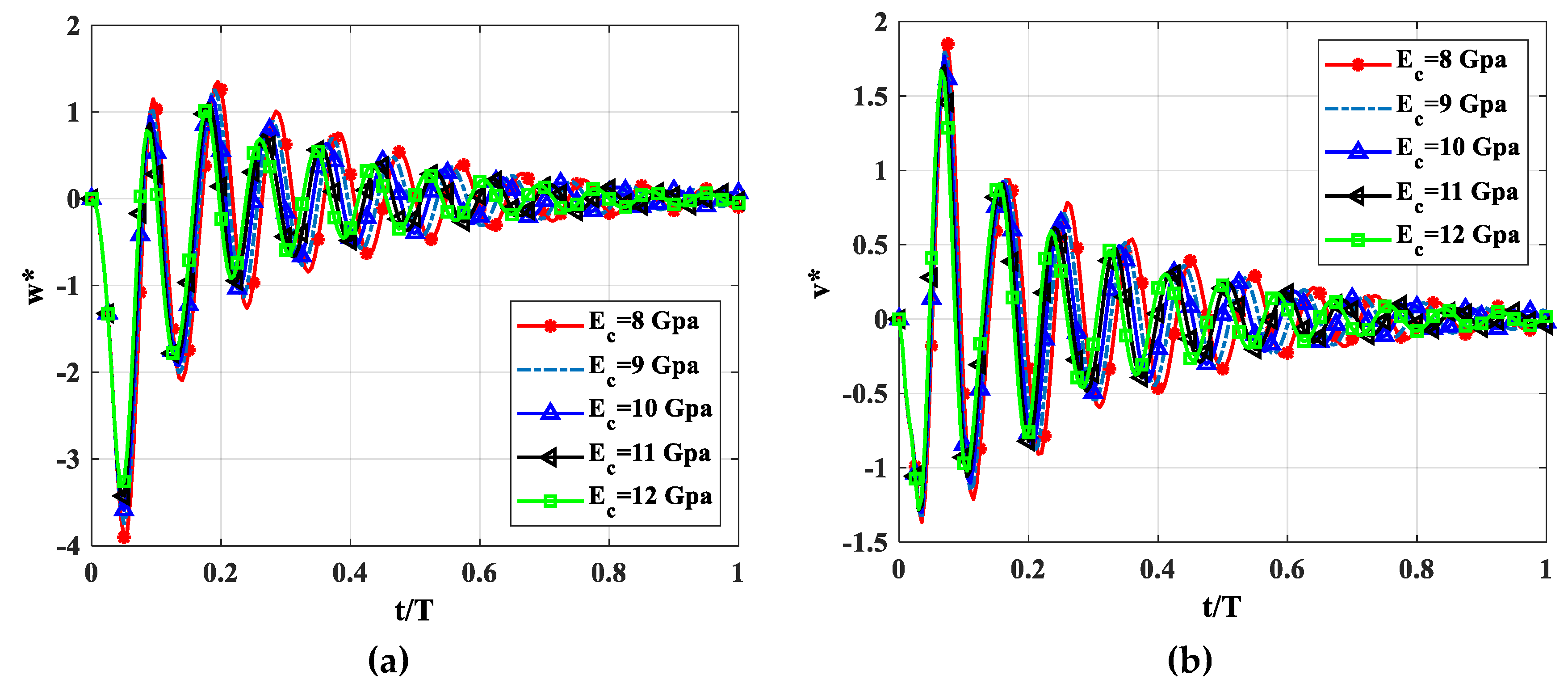
4.2.6. Influence of Modulus of Elasticity

Let us consider a fully simply-supported (SSSS) shell (b = a) with h_c = h/2, h_t = h_b = h/4. The shear modulus of the shear connector is k_s = 50 MPa. The modulus of elasticity of the three layers are E_t = E_b = 12 GPa and E_c = 8, 9, 10, 12 GPa. Nondimensional deflection and velocity of the shell center point are shown in Figure 10, and the maximum deflections and velocities of the shell center point are illustrated in

Table 12. Maximum deflection and velocity of the shell center point over time for different E_c.

Maximum Values	Ec = 8 GPa	Ec = 9 GPa	Ec = 10 GPa	Ec = 12 GPa	Ec = 12 GPa
${\mathrm{w}}_{\max }^{\ast }$	3.9020	3.7494	3.5895	3.4252	3.3031
${\mathrm{v}}_{\max }^{\ast }$	1.3653	1.3375	1.2998	1.2841	1.2792

.

Comment: From the Figure 10 and Table 12, we can find that when modulus of elasticity of the core-layer is increased in a range from 8 to 12 GPa, deflection and velocity of the shell center point are slightly decreased.

5. Conclusions

The finite element method (FEM) is the numerical method for solving problems of engineering and mathematical physics, including the calculation of shell structures. Establishing the balance equation describing the vibration of shell structure is quite simple and it is very convenient for coding on a personal computer (PC). The proposed program is able to analyze the static bending, dynamic response, nonlinear problems, etc., with complicated structures, which are not easy to solve by analytical methods.

Based on the finite element method, we established the equilibrium equation of a triple-layer composite shell with shear connectors subjected to dynamic loads. In this paper, employing of the eight-node isometric element is suitable. To exactly describe the strain field, the displacements of the three-layer shell with shear connectors, and the 13-degrees of freedom element is used, in which the three layers have the same a degree of freedom in the z-direction, and the other 12 degrees of freedom are described as the linear displacement and rotation angle of each layer. Hence, the displacement field and the strain field of each layer can be investigated deeply. We have created the program in the MATLAB environment to investigate effects of various geometrical parameters on free and forced vibrations of shells. To sum up, some main interesting points of this paper are listed in the following statements.

In general, the geometrical parameters effect strongly on free and forced vibrations of the shell; when the shape of the shell is small, the structure gets stiffer.

Based on the numerical results, we realized that for this type of structure, the shear coefficient of the stub plays a very important role. Especially, when the stiffness of the shear coefficient is large enough, this structure seems to be a sandwich shell.

From the above computed results, we suggest that in order to reduce the vibration of such a structure, we should use the middle layer, having the elastic modulus less than other layers, and the thickness of the middle layer 20–30 times larger than the other ones.

We suggest that, in order to reduce the volume of the shell structure subjected to the blast load, we should consider the triple-layer shell with the core layer having a smaller density than the two layers others. Another interesting thing is that the core layer has less stiffener than the other two layers for the displacement response, the velocity is almost unchanged, so we can be flexible in making shells with available materials and different stiffeners.

Based on the achieved numerical results, this paper also leads to further works; for instance, the analysis of FGM structures with shear connectors, buckling problems, the composite plate with shear connectors subjected to both temperature and mechanical loads, and so on.

References

1. Newmark, N.M.; Siess, C.P.; Viest, I.M. Test and analysis of composite beams with incomplete interaction. Proc. Soc. Exp. Stress Anal. 1951, 19, 75–92. [Google Scholar]
2. He, G.; Yang, X. Finite element analysis for buckling of two-layer composite beams using Reddy’s higher order beam theory. Finite Elem. Anal. Des. 2014, 83, 49–57. [Google Scholar] [CrossRef]
3. Xu, R.; Wang, G. Variational principle of partial-interaction composite beams using Timoshenko’s beam theory. Int. J. Mech. Sci. 2012, 60, 72–83. [Google Scholar] [CrossRef]
4. Xu, R.; Wu, Y. Static, dynamic, and buckling analysis of partial interaction composite members using Timoshenko’s beam theory. Int. J. Mech. Sci. 2007, 49, 1139–1155. [Google Scholar] [CrossRef]
5. Nguyen, Q.H.; Hjiaj, M.; Grognec, P.L. Analytical approach for free vibration analysis of two-layer Timoshenko beams with interlayer slip. J. Sound Vib. 2012, 331, 2949–2961. [Google Scholar] [CrossRef]
6. Da Silva, A.R.; Sousa, J.B.M., Jr. A family of interface elements for the analysis of composite beams with interlayer slip. Finite Elem. Anal. Des. 2009, 45, 305–314. [Google Scholar] [CrossRef]
7. Schnabl, S.; Saje, M.; Turk, G.; Planinc, I. Analytical solution of two-layer beam taking into account interlayer slip and shear deformation. J. Struct. Eng. 2007, 133, 886–894. [Google Scholar] [CrossRef]
8. Nguyen, Q.H.; Martinelli, E.; Hjiaj, M. Derivation of the exact stiffness matrix for a two-layer Timoshenko beam element with partial interaction. Eng. Struct. 2011, 33, 298–307. [Google Scholar] [CrossRef]
9. Nguyen, Q.H.; Hjiaj, M.; Lai, V.-A. Force-based FE for large displacement inelastic analysis of two-layer Timoshenko beams with interlayer slips. Finite Elem. Anal. Des. 2014, 85, 1–10. [Google Scholar] [CrossRef]
10. Huang, C.W.; Su, Y.H. Dynamic characteristics of partial composite beams. Int. J. Struct. Stab. Dyn. 2008, 8, 665–685. [Google Scholar] [CrossRef]
11. Shen, X.; Chen, W.; Wu, Y.; Xu, R. Dynamic analysis of partial-interaction composite beams. Compos. Sci. Technol. 2011, 71, 1286–1294. [Google Scholar] [CrossRef]
12. Arvin, H.; Bakhtiari-Nejad, F. Nonlinear free vibration analysis of rotating composite Timoshenko beams. Compos. Struct. 2013, 96, 29–43. [Google Scholar] [CrossRef]
13. Chakrabarti, A.; Sheikh, A.H.; Griffith, M.; Oehlers, D.J. Dynamic response of composite beams with partial shear interaction using a higher-order beam theory. J. Struct. Eng. 2013, 139, 47–56. [Google Scholar] [CrossRef]
14. Chakrabarti, A.; Sheikh, A.H.; Griffith, M.; Oehlers, D.J. Analysis of composite beams with longitudinal and transverse partial interactions using higher order beam theory. Int. J. Mech. Sci. 2012, 59, 115–125. [Google Scholar] [CrossRef]
15. Chakrabarti, A.; Sheikh, A.H.; Griffith, M.; Oehlers, D.J. Analysis of composite beams with partial shear interactions using a higher order beam theory. Eng. Struct. 2012, 36, 283–291. [Google Scholar] [CrossRef]
16. Subramanian, P. Dynamic analysis of laminated composite beams using higher order theories and finite elements. Compos. Struct. 2006, 73, 342–353. [Google Scholar] [CrossRef]
17. Li, J.; Shi, C.; Kong, X.; Li, X.; Wu, W. Free vibration of axially loaded composite beams with general boundary conditions using hyperbolic shear deformation theory. Compos. Struct. 2013, 97, 1–14. [Google Scholar] [CrossRef]
18. Vo, T.P.; Thai, H.-T. Static behavior of composite beams using various refined shear deformation theories. Compos. Struct. 2012, 94, 2513–2522. [Google Scholar] [CrossRef]
19. Tarun, K.; Owen, D.R.J.; Zienkiewicz, O.C. A refined higher-order C0 plate bending element. Compos. Struct. 1982, 15, 177–183. [Google Scholar]
20. Manjunatha, B.S.; Kant, T. New theories for symmetric/unsymmetric composite and sandwich beams with C0 finite elements. Compos. Struct. 1993, 23, 61–73. [Google Scholar] [CrossRef]
21. Yan, J.B.; Zhang, W. Numerical analysis on steel-concrete-steel sandwich plates by damage plasticity model, Materials to structures. Constr. Build. Mater. 2017, 149, 801–815. [Google Scholar] [CrossRef]
22. Carrera, E.; Petrolo, M.; Zappino, E. Performance of CUF Approach to Analyze the Structural Behavior of Slender Bodies. J. Struct. Eng. 2012, 138, 285–297. [Google Scholar] [CrossRef]
23. Carrera, E. Theories and finite elements for multilayered, anisotropic, composite plates and shells. Arch. Comput. Methods Eng. 2002, 9, 87–140. [Google Scholar] [CrossRef]
24. Cinefra, M.; Kumar, S.K.; Carrera, E. MITC9 Shell elements based on RMVT and CUF for the analysis of laminated composite plates and shells. Compos. Struct. 2019, 209, 383–390. [Google Scholar] [CrossRef]
25. Muresan, A.A.; Nedelcu, M.; Gonçalves, R. GBT-based FE formulation to analyse the buckling behaviour of isotropic conical shells with circular cross-section. Thin-Walled Struct. 2019, 134, 84–101. [Google Scholar] [CrossRef]
26. Schardt, R. Verallgemeinerte Technische Biegetheorie: Lineare Probleme; Springer: Berlin/Heidelberg, Germany, 1989. [Google Scholar]
27. Fryba, L. Vibration of Solids and Structures under Moving Loads; Springer: Berlin, Germany, 1999. [Google Scholar]
28. Hoang-Nam, N.; Tan-Y, N.; Ke, V.T.; Thanh, T.T.; Truong-Thinh, N.; Van-Duc, P.; Thom, V.D. A Finite Element Model for Dynamic Analysis of Triple-Layer Composite Plates with Layers Connected by Shear Connectors Subjected to Moving Load. Materials 2019, 12, 598–617. [Google Scholar]
29. Ansari Sadrabadi, S.; Rahimi, G.H.; Citarella, R.; Shahbazi Karami, J.; Sepe, R.; Esposito, R. Analytical solutions for yield onset achievement in FGM thick walled cylindrical tubes undergoing thermomechanical loads. Compos. Part B Eng. 2017, 116, 211–223. [Google Scholar] [CrossRef]
30. Bathe, K.J. Finite element Procedures; Prentice-Hall International Inc.: Upper Saddle River, NJ, USA, 1996. [Google Scholar]
31. Wolf, J.P. Dynamic Soil-Structure Interaction; Prentice-Hall Inc.: Upper Saddle River, NJ, USA, 1985. [Google Scholar]
32. Reddy, J.N. Mechanics of Laminated Composite Plate and Shell, 2nd ed.; CRC Press: Boca Raton, FL, USA, 2004. [Google Scholar]
33. Qian, L.F. Free and Forced Vibrations of Thick Rectangular Plates using Higher-Order Sheara and Normal Deformable Plate Theory and Meshless Petrov-Galerkin (MLPG) Method. CMES 2003, 5, 519–534. [Google Scholar]
Figure 1. The model of three-layer composite shell with shear connectors, (a) shell model with shear connectors, and (b) finite element model.
Symmetry 11 00527 g001
Figure 2. Degrees of freedom of the node in the eight-node shell element.
Symmetry 11 00527 g002
Figure 3. Algorithm flowchart of Newmark solving the dynamic response problem of the shell.
Symmetry 11 00527 g003
Figure 4. The deflection of the centroid point of the plate overtime.
Symmetry 11 00527 g004
Figure 5. Effect of length-to-high ratio a/h on the non-dimensional deflection and velocity of the centroid point. (a) Nondimensional deflection w* versus time; and (b) nondimensional velocity v* versus time.
Symmetry 11 00527 g005
Figure 6. Effect of hc/ht ratio on the non-dimensional deflection and velocity of the centroid point. (a) Nondimensional velocity w* versus time; (b) Nondimensional velocity v* versus time; (c) Nondimensional deflection u c versus time; (d) Nondimensional deflection v c versus time.
Symmetry 11 00527 g006
Figure 7. Effect of length-to-width ratio a/b on the non-dimensional deflection and velocity of the centroid point. (a) Nondimensional deflection w* versus time; and (b) nondimensional velocity v* versus time.
Symmetry 11 00527 g007
Figure 8. Effect of shear coefficient of stub on the non-dimensional deflection and velocity of the centroid point. (a) Nondimensional deflection w* versus time; and (b) nondimensional velocity v* versus time.
Symmetry 11 00527 g008
Figure 9. Dynamic deflections of center point of the plate versus time for different ρc. (a) Nondimensional deflection w* versus time, and (b) nondimensional velocity v* versus time.
Symmetry 11 00527 g009
Figure 10. Dynamic deflections of center point of the shell over time with different Ec. (a): Nondimensional deflection w* versus time, and (b) nondimensional velocity v* versus time.
Symmetry 11 00527 g010