Towards Infinite Tilings with Symmetric Boundaries

Abstract

Large-time coarsening and the associated scaling and statistically self-similar properties are used to construct infinite tilings. This is realized using a Cahn–Hilliard equation and special boundaries on each tile. Within a compromise between computational effort and the goal to reduce recurrences, an infinite tiling has been created and software which zooms in and out evolve forward and backward in time as well as traverse the infinite tiling horizontally and vertically. We also analyze the scaling behavior and the statistically self-similar properties and describe the numerical approach, which is based on finite elements and an energy-stable time discretization.

1. Introduction

At first-order phase transitions, coexisting macroscopic domains of different phases emerge from small fluctuations of a homogeneous phase. Late stages of this process are often dominated by the motion of the interfaces separating the domains. Considering this large-time coarsening behavior, i.e., the growth of a characteristic length scale $l(t)$ as $t\to \infty$ determines important characteristics of the dynamics and led to the identification of several universality classes of domain growth. We are here concerned with conserved order parameters, for which the expected behavior is $l(t)\sim t^{1/3}$, which results from the scale invariance of the Mullins–Sekerka system $x\to \lambda x$, $t\to {\lambda }^{3}t$. Rigorous results exist for an upper bound for $l(t)$, stating that microstructures cannot coarsen faster than the similarity rate [1]. As there are non-generic configurations, e.g., stripe domains with zero curvature which are stable, lower bounds cannot be expected within a deterministic framework. Besides this scaling law, solutions with random initial data are also believed to be statistically self-similar in this large-time regime. Numerical studies based on a Cahn–Hilliard equation and related coarse-grained theories indicate that the approach of the large-time regime with the statistically self-similar structures might be very slow [2]. To explore these regimes numerically thus requires large length and time scales, which limits the accessible sample size. We are here interested in these statistically self-similar structures, which have been used for various art and design projects, e.g., [3]. Here, we would like to explore very large, in principle infinite, samples. To tackle such a system we consider, instead of one huge simulation, many moderately sized domains with different initial data, and require the boundaries to match. If appropriately done, this will allow construction of large (infinite) tilings which are statistically self-similar. With a random arrangement of finitely many computed structures, the impression of an infinite tiling with no recurrence could be achieved. For this impression, the boundary conditions at the computational domains are crucial. They are described in detail in Section 4 together with the finite-element approach to solve the Cahn–Hilliard equation. In Section 2 we show various results, among other things a computer program which allows navigation through space and time of an infinitely extended structure. We further discuss improvements and outline possible applications. In Section 3, we discuss scaling and self-similar properties.

2. Results

As the underlying model for phase transitions with a conserved order parameter we consider a Cahn–Hilliard equation

$${\partial }_t\varphi =\gamma \Delta \mu ,\mu =-{ϵ}^2\Delta \varphi +B^{\prime }(\varphi );$$

(1)

see Section 4 for details. First, we consider coarsening in a rectangular cuboid using standard boundary conditions $\mathbf{n}·\nabla \varphi =\mathbf{n}·\nabla \mu =0$ on $\partial \Omega$. Figure 1 shows snapshots of the results within the large-time regime, visualized in various ways. The interface area is minimized, and the structure thus coarsens in time. To analyze this in a statistical manner requires either a larger domain or more samples. Our idea is to combine both by using samples which are distinct from each other but fit together to form a large and extendable structure. The boundary conditions in the current setting enforce the level lines of the interface to be perpendicular to $\partial \Omega$. They in addition do not fit to each other and thus do not allow combination of different samples. To overcome these limitations, we consider a smaller domain, again a rectangular cuboid and the boundary conditions introduced in Section 4 which specify the values of $\varphi$ and the normal flux $\nabla \varphi ·\mathbf{n}$ such that opposite sides match. The first approach only has two distinct boundaries, $N=2$. Figure 2 shows four samples, all obtained with different initial conditions and considered at the same time instance. The structures fit together and any translation in x- or y-direction by the width of the domain will also fit. The individual figures are provided in SI as Figures S1–S4; print them and try it out. The figures are part of an art project, $M=100$ individual samples have been computed and printed on Alu-Dibond in size 20 cm × 20 cm, creating a 200 cm × 200 cm figure which can be displayed in $100!\approx 9.332622·{10}^{157}$ variations.

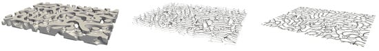
Figure 1. Typical structure within the large-time regime, visualized as $\varphi =1$ in $\Omega$, $\varphi =0.5$ at $z=0.01$, 0.13, 0.25, 0.37, 0.49 and $\varphi =0.5$ at $z=0.01$, 0.13, 0.25, 0.37, 0.49 projected to $z=0$, from left to right. The boundary conditions are $\mathbf{n}·\nabla \varphi =\mathbf{n}·\nabla \mu =0$ on $\partial \Omega$. The corresponding videos of the coarsening process are provided in SI as Videos S5–S7.

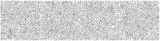
Figure 2. Four samples with identical boundaries but distinct inner structure. The samples are translational invariant in x- and y-direction.

Even if the inner structure is unique for each tile, the boundaries in x- and y-direction are the same and recurrences are visible. To improve on this issue, we consider a second approach, which is less flexible in terms of arrangement of samples but minimizes possible recurrences. As a compromise of computational cost and visual impression we consider tilings with $N=10$ different boundary conditions. This improves the impression of a tiling with no recurrence since systematic recurrence in a row, a column, or diagonally can be avoided by careful assembly of the tiles. Repetitions do not only appear less frequently but also in a pattern that is much less obvious. To see this recurrence without knowing the construction process and explicitly searching for them is almost impossible. We consider two different internal realizations each, leading to $M=10$. Within the proposed pattern determined by the boundary conditions the inner realization are randomly chosen to construct an infinite tiling, where recurrences are almost invisible.

A software is developed to visualize the infinite structure. We consider visualizations with five projected level lines of the interface. The software allows zooming in and out, evolve forward and backward in time as well as traverse the infinite tiling horizontally and vertically. Figure 3 shows some screenshots, starting from an early time instant and a low zoom factor (a), going to a late-time instant of this setting (b), zooming into the structure (c), evolving along a trajectory in space and time, which keeps the interface area constant (d), and going back to the initial state (a). Videos of the journey through space and time are provided in SI as Videos S8 and S9.

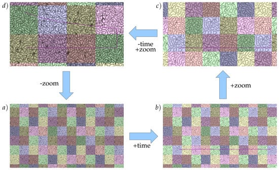
Figure 3. Screenshots of the visualization software, here in addition color-coded according to the individual tiles used. The dark magenta lines indicate the user-interaction. Moving the mouse horizontally evolves time, moving it vertically zooms in and out.

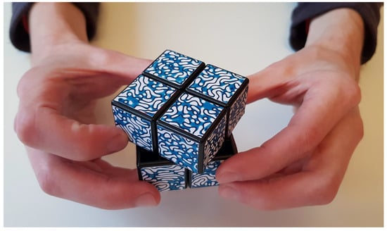
As the proposed approach is in principle not restricted to rectangular cuboidal domains various possibilities for applications can be imagined. Besides wallpaper design, they range from fashion design with individualized clothes to camouflage patterns of automotive prototypes. Here, we highlight a more entertaining application, a Rubik’s cube which always fits, but has 24 different fields; see Figure 4.

Figure 4. A Rubik’s cube which always fits even if all tiles are different. A video is provided in SI as Video S10.

3. Discussion

We now explore the scaling properties and the statistically self-similar behavior of the constructed infinite tiling. The theoretically scaling behavior $l(t)\sim t^{1/3}$ of a characteristic length scale is tested by computing the interface area of each tile over time. The interface is thereby represented as the level-surface $\varphi =0$. In addition, we also compute the length of the interface of the level line at $z=0.25$, which is used for visualization. Figure 5 shows the results over time, which are averaged over all individual realizations of tiles.

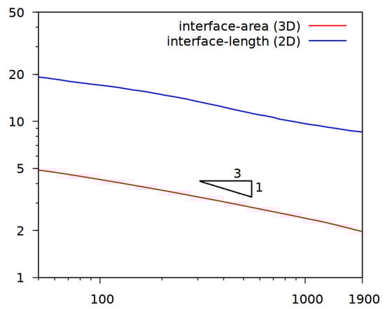
Figure 5. Development of the interface area of the 3D-structure and the interface-length of a slice through the center of the domain over time, averaged for all tiles.

The results lead to a scaling exponent which is below the upper bound of $1/3$. The slope is not constant, but on average equal for the two measures and approximately 0.26. There are different reasons for this lower value, either the structure has not reached the late-time behavior for which the theoretical scaling behavior is expected, or the considered domain with the zero-flux boundary conditions on top and bottom favor parallel structures and thus prevent coarsening. The limitation of our approach, to combine several tiles and to compute them separately, should also be mentioned. This approach only allows the consideration of coarsening up to a length scale of the size of a tile. For larger times, the approach is no longer valid. However, even if the theoretical scaling law could not be shown computationally, statistical self-similarity still might be possible. Statistical self-similarity can already be expected from a randomly chosen sample. We consider the middle slice at an early time instant, its coarsening and subsequent zooming-out in Figure 6. Instead of the interface line the two phases are rendered in black and white. When the coarse structure is zoomed out to a degree where the interface-length matches that of the earlier timestep, both structures are visually similar (see Figure 6a,c). To quantify this, we compute for each row and column of pixels the distance between two interfaces. This is done for all samples and plotted for different times in Figure 7.

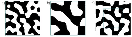
Figure 6. Middle slice of the domain in an early time instance (a), a later point in time (b) and the later time-point zoomed out until the interface-length equals that of the early one (c). In the last image the unzoomed region is framed to indicate the level of zoom applied.

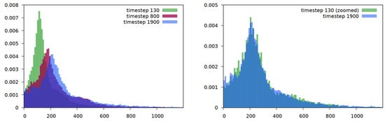
Figure 7. Left: density-histograms of the distances between interfaces for three selected timesteps (all tiles combined). Right: a square subregion of timestep 130 is considered which, after zooming to the size of a full tile, has the same interface area as timestep 1900. The histograms match almost exactly, which computationally indicates the statistically self-similar structure.

Even if the theoretically predicted scaling law $l(t)\sim t^{1/3}$ could not be computationally shown, the large-scale simulations, which run for each tile on a high-performance computer, reproduce the predicted statistical self-similarity. The huge structure, which results as an arrangement of individual tiles, would not have been possible to simulate on the available hardware. The approach fulfills two goals, it provides enough statistics to analyze scaling and statistical self-similarity and it allows the generation of aesthetically appealing tilings with almost invisible recurrences, which can be infinitely extended.

4. Materials and Methods

The Cahn–Hilliard equation [4] is a fourth order partial differential equation resulting as a $H^{-1}$ gradient flow of a Ginzburg-Landau energy

$$\mathcal{E}[\varphi ]={\int }_{\Omega }\gamma \left(\frac{{ϵ}^2}{2}{|\nabla \varphi |}^2+B(\varphi )\right)d\Omega ,$$

(2)

where $\Omega$ is a bounded domain, $ϵ$ a positive parameter determining the width of the diffuse interface, $\gamma$ the surface energy, here considered as a positive constant, and $B(\varphi )=\frac{1}{4}{(1-{\varphi }^2)}^2$ a double well potential. The resulting equation reads

$${\partial }_t\varphi =\gamma \Delta \mu ,\mu =-{ϵ}^2\Delta \varphi +B^{\prime }(\varphi )$$

(3)

and converges for $ϵ\to 0$ to the Mullins–Sekerka problem [5]; see Ref. [6].

Various numerical approaches have been proposed to solve the equation efficiently. We consider a convexity splitting approach, e.g., [7,8,9,10,11]. The idea is to split the double well potential $B(\varphi )=B_c(\varphi )-B_e(\varphi )$, such that both parts are convex and to consider the time discretization as

$$d_{\tau }{\varphi }^{n+1}=\gamma \Delta {\mu }^{n+1},{\mu }^{n+1}=-{ϵ}^2\Delta {\varphi }^{n+1}+B_c^{\prime }({\varphi }^{n+1})-B_e^{\prime }({\varphi }^n),$$

(4)

with discrete time derivative $d_{\tau }{\varphi }^{n+1}=({\varphi }^{n+1}-{\varphi }^n)/{\tau }_n$. The resulting scheme is unconditionally energy stable, unconditionally solvable and converges optimally in the energy norm [9]. To solve the above systems, we consider a linearization of $B_c^{\prime }({\varphi }^{n+1})\approx B_c^{\prime }({\varphi }^n)+B_c^{″}({\varphi }^n)({\varphi }^{n+1}-{\varphi }^n)$. We further consider adaptive mesh refinement according to criteria related to the position of the diffuse interface, here $\nabla \varphi$, to ensure a resolution of approximately five grid points across the interface and a coarser mesh elsewhere; see Figure 8.

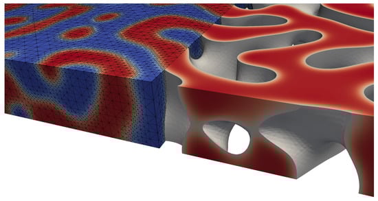
Figure 8. Typical structure, highlighting one of the two phases and the adaptively refined mesh along the diffuse interface.

The resulting linear system is solved in parallel using a block-preconditioner, see [12,13], and the iterative solver FGMRES. All problems are implemented in the adaptive finite-element toolbox AMDiS [14,15]. The considered parameters are $ϵ=0.01$ and $\gamma =1.0$ and as computational domain rectangular cuboid $\Omega =(0,L)x(0,L)x(0,l)$ with $l=0.2$ and $L=2.0$ for the larger and $L=1.0$ for the smaller domain and boundaries ${\Gamma }^{top}$, ${\Gamma }^{bottom}$, ${\Gamma }^0$ and ${\Gamma }^1={\bigcup }_{i=1}^4{\Gamma }^{1,i}$, see Figure 9. The number of grid points on the larger domain reduces from approx. 2.95 million at the beginning to approx. 1.95 million at the final configuration.

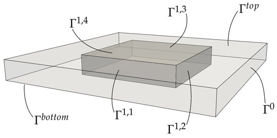
Figure 9. Geometric setting and boundaries.

As initial condition we consider white noise around the mean value $\varphi =0$. At ${\Gamma }^{top}$ and ${\Gamma }^{bottom}$ we specify zero-flux boundary conditions for $\varphi$ and $\mu$. We first consider the larger domain with zero-flux boundary conditions for $\varphi$ and $\mu$ also on ${\Gamma }^0$. In this setting the finite-element formulation in each time step reads: Find ${\varphi }^{n+1},{\mu }^{n+1}\in V_h$ such that $\forall \eta ,\xi \in V_h$

$$\begin{array}{ccc}\hfill {\int }_{\Omega }{d}_{\tau }{\varphi }^{n+1}\eta dx+\gamma {\int }_{\Omega }\nabla {\mu }^{n+1}·\nabla \eta dx& =& 0\hfill \end{array}$$

(5)

$$\begin{array}{ccc}\hfill {\int }_{\Omega }{\mu }^{n+1}\xi dx-{ϵ}^2{\int }_{\Omega }\nabla {\varphi }^{n+1}·\nabla \xi dx-{\int }_{\Omega }{B}_c^{\prime }({\varphi }^{n+1})\xi dx& =& -{\int }_{\Omega }{B}_e^{\prime }({\varphi }^n)\xi dx,\hfill \end{array}$$

(6)

with $V_h=\{v\in C^0(\Omega )|v_{|T}\in P^1(T)\forall T\in \mathcal{T}\}$ the space of piecewise linear Lagrange elements and triangulation $\mathcal{T}$. In each time step we extract ${\varphi }_1^{n+1}={\varphi }^{n+1}$ and $\mathbf{n}·\nabla {\varphi }_1^{n+1}=\mathbf{n}·\nabla {\varphi }^{n+1}$ along the inner boundary ${\Gamma }^1$. These data are going to be used in the subsequent computations in the smaller domain as boundary conditions on ${\Gamma }^1$. The finite-element formulation now reads in each time step: Find ${\varphi }^{n+1}\in V_{h,{\Gamma }^1,{\varphi }_1}$ and ${\mu }^{n+1}\in V_h$ such that $\forall \eta \in V_{h,{\Gamma }^1,0}$ and $\forall \xi \in V_h$

$$\begin{array}{ccc}\hfill {\int }_{\Omega }{d}_{\tau }{\varphi }^{n+1}\eta dx+\gamma {\int }_{\Omega }\nabla {\mu }^{n+1}·\nabla \eta dx& =& 0\hfill \end{array}$$

(7)

$$\begin{array}{ccc}\hfill {\int }_{\Omega }{\mu }^{n+1}\xi dx-{ϵ}^2{\int }_{\Omega }\nabla {\varphi }^{n+1}·\nabla \xi dx-{\int }_{\Omega }{B}_c^{\prime }({\varphi }^{n+1})\xi dx& =& -{\int }_{\Omega }{B}_e^{\prime }({\varphi }^n)\xi dx-{ϵ}^2{\int }_{{\Gamma }^1}\mathbf{n}·\nabla {\varphi }_1\xi ds,\hfill \end{array}$$

(8)

with $V_{h,{\Gamma }^1,\alpha }=\{v\in C^0(\Omega )|v_{|T}\in P^1(T)\forall T\in \mathcal{T},v=\alpha$ on ${\Gamma }^1\}$.

For different initial data this leads to different solutions with common boundary conditions. However, to construct tilings, they also must match, which is not yet guaranteed. To fulfill this requirement, we proceed in two different ways. The first approach considers only one computation on the larger domain and uses the extracted values and fluxes ${\varphi }_1^{n+1}$ and $\mathbf{n}·\nabla {\varphi }_1^{n+1}$ at ${\Gamma }^1$ only from two sides ${\Gamma }^{1,1}$ and ${\Gamma }^{1,2}$ ($N=2$) and specifies them also on the opposite sides for the computations on the smaller domain. For M different initial conditions this generates M individual samples which match with each other at the boundaries if translated by the domain size in x- or y-direction. This leads to a very flexible arrangement of the samples but has the drawback of frequent recurrence at the boundaries.

The second approach also begins with a computation on the larger domain with boundary ${\Gamma }^0$ but subsequent computations are performed on intermediate domains that extend to the bounds of ${\Gamma }^0$ in directions where a fresh structure is desired at the boundary and are restricted to the bounds of the smaller domain ${\Gamma }^1$ in directions where the structure is to be continued from an already existing neighbor tile by using its stored values and fluxes ${\varphi }_1$ and $\mathbf{n}·\nabla {\varphi }_1$ at ${\Gamma }^1$. This requires small modifications of the finite-element formulation in Equations (7) and (8) using only parts of ${\Gamma }^1$ instead of the whole inner boundary. When enough samples are computed to define all N boundary sides the remaining samples are computed on ${\Gamma }^1$ with all sides fixed by boundary conditions from earlier computations.

The most simple setup meeting our design-goal of non-obvious recurrence of boundaries requires five different tiles $A_0$, $B_0$, $C_0$, $D_0$ and $E_0$ which can be assembled into a row that matches the same row displaced by a few tiles above and below. Then, five rows of five tiles each form a square which can be continued in all directions indefinitely (see Figure 10c). This setup allows for ten unique boundary sides $s_1$ through $s_{10}$ (see Figure 11). Inside our 5 × 5 square of tiles recurrences do not occur in a row, a column, or diagonally, which would not be possible with a smaller number of unique tiles. With only two or three different tiles, repetitions would have to occur at least diagonally (see Figure 10a) and with four different tiles it is only possible to build a unique 4 × 2 rectangle without diagonal repetitions (see Figure 10b).

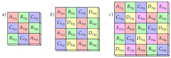
Figure 10. (a) Layout of $3\times 3$ tiles: diagonal recurrence cannot be avoided. (b) Layout of $4\times 4$ tiles: the bottom two rows are duplicates of the top two; all other arrangements would yield diagonal recurrence. (c) Layout of $5\times 5$ tiles: recurrences in non-obvious pattern.

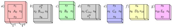
Figure 11. Initial five tiles and their connecting boundary sides. a) Tile $A_0$ is simulated on ${\Gamma }^0$; b,d) $B_{tmp}$ and $C_{tmp}$ are intermediate steps in preparation of $B_0$ and $C_0$, respectively; c,e,f,g) tiles $B_0$ through $E_0$ are simulated on domains that extend ${\Gamma }^1$ towards ${\Gamma }^0$ only in directions where fresh boundary data is required, the other boundaries are fixed.

On the macroscopic scale our pattern still has obvious repetitions since we need to continue the same square of 5 × 5 tiles in all directions to form the infinite tiling. To remedy this problem, we generate variants of our five initial tiles $A_1$, $B_1$, $C_1$, $D_1$ and $E_1$ which exactly copy the boundaries of their respective prototype with index zero but differ on the inside. Now, in our infinite tiling each tile of a specific prototype is replaced randomly with either the original 0-variant or the new 1-variant of that type. With only two variants per type we already allow for more than 33 million ($2^{25}$) distinct squares of 5 × 5 tiles. For our interactive visualization software, we settled with these $M=10$ tiles due to memory-constraints. However, for printed realizations such as wallpapers, further variants could be computed, making it even harder to spot recurrences.

The initial five tiles must be computed consecutively since their boundaries depend on each other. Starting with $A_0$ we have no constraints yet and thus the simulation yields four fresh boundary sides. The simulation domain ${\Gamma }^0$ exceeds the region of interest ${\Gamma }^1$ in all four connecting directions because we need to avoid the level lines always being perpendicular to the boundary of ${\Gamma }^1$ (Figure 11a).

As a next step we simulate a temporary tile $B_{tmp}$ to prepare the run for $B_0$. Obviously, tile $B_0$ has to match $A_0$’s right-hand side boundary ($s_2$ in Figure 11b) at its own left-hand side. However, this is not the only constraint. Our 5 × 5 layout requires that $B_0$ meets $A_0$ also in its top-right corner (see Figure 10c). Thus, in our temporary step besides fixing the left boundary we also fix the top boundary with a mirrored version $s_3^m$ of the data from $A_0$’s bottom side. The mirroring is required because the top-right corner of $B_0$ must conform to the bottom-left corner of $A_0$. The simulation domain for $B_{tmp}$ exceeds the region of interest only in two directions: bottom and left, where we obtain data for two fresh boundary sides (Figure 11b). Now we are ready to compute our second tile $B_0$. We fix the right, bottom and left boundaries with data from our previous two simulations and this time leave the top-side unconstrained to obtain a fresh boundary that is only fixed at the two corners where it will match tile $A_0$ (Figure 11c).

For tile $C_0$ we require another preliminary run $C_{tmp}$ to fix the bottom-left corner where it meets $A_0$. We use the mirrored top-side $s_1^m$ of $A_0$ at $C_{tmp}$’s bottom to account for that and fix the left and top sides where $C_0$ shares sides with $B_0$ and $A_0$. Only at the left-hand side we obtain a fresh set of boundary-data (Figure 11d). For $C_0$ we release the bottom-constraint of $C_{tmp}$ and obtain another fresh boundary (Figure 11e). The last tile with a fresh boundary is $D_0$. All sides, except the right-hand side one, are already constrained by previous computations (Figure 11f). For $E_0$ all four sides are fully predetermined (Figure 11g). We need to simulate it only for its interior.

All variant-tiles $A_1$ through $E_1$ (and further ones if desired) can now be computed in parallel since their boundaries are already known. They are all restricted to ${\Gamma }^1$ and do not require extraction of boundary-values and -fluxes, hence are computationally less expensive than the initial runs.

References

- Kohn, R.; Otto, F. Upper bounds on coarsening rates. Commun. Math. Phys. 2002, 229, 375–395. [Google Scholar] [CrossRef]
- Garcke, H.; Niethammer, B.; Rumpf, M.; Weikard, U. Transient coarsening behaviour in the Cahn-Hilliard model. Acta Mater. 2003, 51, 2823–2830. [Google Scholar] [CrossRef]
- Stenger, F.; Voigt, A. Interactive evolution of a bicontinuous structure. Leonardo 2019. [Google Scholar] [CrossRef]
- Cahn, J.; Hilliard, J. Free energy of a nonuniform system .1. interfacial free energy. J. Chem. Phys. 1958, 28, 258–267. [Google Scholar] [CrossRef]
- Mullins, W.; Sekerka, R. Morphological stability of a particle growing by diffusion or heat flow. J. Appl. Phys. 1963, 34, 323–329. [Google Scholar] [CrossRef]
- Pego, R.L. Front migration in the nonlinear Cahn-Hilliard equation. Proc. R. Soc. A 1989, 422, 261–278. [Google Scholar] [CrossRef]
- Eyre, D.J. Unconditionally Gradient Stable Time Marching the Cahn-Hilliard Equation. MRS Online Proc. Libr. Arch. 1998, 1686–1712. [Google Scholar] [CrossRef]
- Bertozzi, A.L.; Esedoglu, S.; Gillette, A. Inpainting of binary images using the Cahn-Hilliard equation. IEEE Trans. Image Process. 2007, 16, 285–291. [Google Scholar] [CrossRef] [PubMed]
- Glasner, K.; Orizaga, S. Improving the accuracy of convexity splitting methods for gradient flow equations. J. Comput. Phys. 2016, 315, 52–64. [Google Scholar] [CrossRef]
- Diegel, A.; Wang, C.; Wise, S. Stability and convergence of a second-order mixed finite element method for the Cahn–Hilliard equation. IMA J. Numer. Anal. 2016, 36, 1867–1897. [Google Scholar] [CrossRef]
- Backofen, R.; Wise, S.; Salvalaglio, M.; Voigt, A. Convexity splitting in a phase field model for surface diffusion. Int. J. Numer. Anal. Mod. 2019, 16, 192–209. [Google Scholar]
- Boyanova, P.; Do-Quang, M.; Neytcheva, M. Efficient preconditioners for large scale binary Cahn-Hilliard models. Comput. Meth. Appl. Math. 2012, 12, 1–22. [Google Scholar] [CrossRef]
- Praetorius, S.; Voigt, A. Development and analysis of a block-preconditioner for the phase-field crystal equation. SIAM J. Sci. Comput. 2015, 37, B425–B451. [Google Scholar] [CrossRef]
- Vey, S.; Voigt, A. AMDiS: Adaptive multidimensional simulations. Comput. Vis. Sci. 2007, 10, 57–67. [Google Scholar] [CrossRef]
- Witkowski, T.; Ling, S.; Praetorius, S.; Voigt, A. Software concepts and numerical algorithms for a scalable adaptive parallel finite element method. Adv. Comput. Math. 2015, 41, 1145–1177. [Google Scholar] [CrossRef]
© 2019 by the authors. Licensee MDPI, Basel, Switzerland. This article is an open access article distributed under the terms and conditions of the Creative Commons Attribution (CC BY) license (http://creativecommons.org/licenses/by/4.0/).