Article

Effectiveness of Nature-Inspired Algorithms using ANFIS for Blade Design Optimization and Wind Turbine Efficiency

1
Department of Mechanical Engineering, Faculty of Engineering, University of Malaya, 50603 Kuala Lumpur, Malaysia
2
Department of Mechatronics Engineering, Kulliyyah of Engineering, International Islamic University Malaysia, 53100 Gombak, Selangor, Malaysia
*
Author to whom correspondence should be addressed.
Symmetry 2019, 11(4), 456; https://doi.org/10.3390/sym11040456
Submission received: 8 February 2019 / Revised: 19 March 2019 / Accepted: 26 March 2019 / Published: 1 April 2019

Abstract

:
Blade design of the horizontal axis wind turbine (HAWT) is an important parameter that determines the reliability and efficiency of a wind turbine. It is important to optimize the capture of the energy in the wind that can be correlated to the power coefficient ( C p ) of HAWT system. In this paper, nature-inspired algorithms, e.g., ant colony optimization (ACO), artificial bee colony (ABC), and particle swarm optimization (PSO) are used to search for the blade parameters that can give the maximum value of C p for HAWT. The parameters are tip speed ratio, blade radius, lift to drag ratio, solidity ratio, and chord length. The performance of these three algorithms in obtaining the optimal blade design based on the C p are investigated and compared. In addition, an adaptive neuro-fuzzy interface (ANFIS) approach is implemented to predict the C p of wind turbine blades for investigation of algorithm performance based on the coefficient determination (R2) and root mean square error (RMSE). The optimized blade design parameters are validated with experimental results from the National Renewable Energy Laboratory (NREL). It was found that the optimized blade design parameters were obtained using an ABC algorithm with the maximum value power coefficient higher than ACO and PSO. The predicted C p using ANFIS-ABC also outperformed the ANFIS-ACO and ANFIS-PSO. The difference between optimized and predicted is very small which implies the effectiveness of nature-inspired algorithms in this application. In addition, the value of RMSE and R2 of the ABC-ANFIS algorithm were lower (indicating that the result obtained is more accurate) than the ACO and PSO algorithms.

1. Introduction

Renewable energy, such as wind energy, biomass energy, hydro energy, and solar energy have been extensively harnessed and exploited during the last decade because of environmental concerns. The most promising source of renewable energy is wind energy due to the factor of low cost in comparison with other sources of renewable energy, such as solar energy and biomass energy, etc. [1,2]. Wind energy is harnessed via the use of a wind turbine system that converts mechanical energy into electrical energy by using a generator. It is classified into various types of systems, such as constant and variable speed systems, power controlling systems, and off grid or on grid [3] systems. Based on the rotation of the axis, there are two types of wind turbines such as the vertical axis wind turbine (VAWT) and the horizontal axis wind turbine (HAWT). In this paper, the HAWT blades are the main concern.
The power coefficient of the blades, which can be defined as the capture capability of efficiency, is the most basic index of wind energy [4]. Design parameters selections are critical for optimization of wind turbine performance. Various parameters influence the energy production of wind turbines, such as, rotor rotational velocity, wind speed, and blade pitch angle [5,6]. For the power coefficient optimization of wind turbine blades, the influence of lift to drag ratio, blade radius, tip-speed ratio, solidity ratio, and the chord length of the blade has been widely investigated. Besides, nature-inspired algorithms (ACO, ABC, and PSO) have also been used in various wind turbine applications.
Eroglu and Ulusam [7] determined the wind farm layout using ACO. They found maximum energy output that considered wake loss, wind turbine location, and wind direction. Fuchs and Gjengedal [8] applied ACO for the necessary time step resolution in a transmission expansion and wind power integration in the Nordic area. They determined the average and peak values for power production from wind technology. Jovanovi et al. [9] focused on maximum segregating of computed graphs of supply and demand. For the optimization, they used ACO and found that the error was less than 5% in comparison with the optimal solutions. Abd-Allah et al. [10] investigated the lightning point in wind turbine farm as lighnting is harmful to wind turbine farm. They used ACO to search for the sensitive points in wind farm. Mustafar et al. [11] studied the loss of reduction of the transformer tap setting to control reactive power using ACO technique.
In the last few years, artificial bee colony (ABC) has massively been studied for a complex problem, modeling, and optimization. The ABC algorithm is not only used in optimization but also for prediction and control. Delgarm et al. [12] determined the performance of energy building using the multi-objective artificial bee colony optimization approach. In addition, Song et al. [13] used an improved ABC algorithm to optimize the combustion of a boiler to consider N O x emission. Ebrahim et al. [14] used the ABC algorithm for proportional integral derivative (PID) controller parameters optimization for speed control of an AC driver. Derakhshan et al. [15] optimized the wind turbine blade shape to determine the aerodynamic performance of blades. Habbi [16] proposed a fuzzy logic system that was self-generated by the ABC algorithm. Based on the above reviews, the ABC algorithm is vastly used for complex problem solving due to its excellent search capability.
Many researchers have also been using the PSO algorithm for location optimization. Safaei et al. [17] proposed the new two-step PSO algorithm for the placement of wind turbine generators for maximum allowable capacity and minimizing power loss in wind turbines. Wind turbine placement at a wind farm was optimized by Wan et al. [18]. Pookpunt and Ongsaku [19] used the binary PSO for wind turbine optimum placement at a wind farm. The size optimization of the hybrid system was determined by PSO [20].
ANFIS is one kind of neural network that shows better learning and estimation capabilities [21]. In the power coefficient prediction or estimation, there are various forms of artificial intelligence. Artificial neural networks (ANN) are user-friendly tools which can learn the mathematical mapping between input and output variables of a nonlinear system. Dalibor and Zarko [22] applied adaptive neuro-fuzzy for the power coefficient estimation. Tip-speed ratio and pitch angle were considered for the power coefficient estimation. They found that the optimal power coefficient was around 0.36. Rajakumar and Ravindran [5] determined the power coefficient and lift and drag coefficient for various airfoil (NASA) using computational fluid dynamics. They showed that the power coefficient level was higher when the drag coefficient was set to zero and the correction of tip loss factor was set to be a constant. Shahaboddin and Dalibor [23] used support vector regression (SVR) based on kernel function for estimating power coefficient and minimizing the generalization error bound. They found similarities in the results of ANFIS and ANN. Sedaghat and Mirhosseini [24] implemented blade element momentum theory (BEM) for a power coefficient of 300 kW in HAWT technology in the province of Semman in Iran. They obtained the maximum power coefficient of 0.51 when the tip-speed ratio was up to its optimum value of 10.
In summary, there is no particular study which focuses on the optimization of the power coefficient wind turbine blades by using three algorithms. The study aims to find the most appropriate blades parameters that provide the maximum power coefficient using ACO, ABC, and PSO. An ANFIS is used to investigate the effectiveness of these nature-inspired algorithms by comparing the results predicted from ANFIS with the results obtained from the nature-inspired algorithm [25]. An endeavor is prepared for retrieving the correlation between C p and the best combination of optimized blade parameters such as lift and drag ratio, blade radius, tip speed ratio, solidity ratio, and chord length of the blade of HAWTs.

2. Power Coefficient of Horizontal Axis Wind Turbine Blade

The progress of the present commercial wind power generator has been continuously moving forward to the latest megawatt (MW) turbine. For HAWTs, parameter selection is challenging. The production of wind turbine power is influenced by various fixed parameters, such as wind velocity, the chord length of blades, rotor diameter, and lift to drag ratio, etc. [4]. There are two goals of the design of a HAWT, i.e., optimizing and estimating the power coefficient [26]. Recently, attention has been placed on a rotor of wind turbine design for maximum aerodynamic performance [27,28,29]. The mechanical power equation for a HAWT can be written as
P m e c h a n i c a l = 0.5   ρ   C p A s V w 3
where air density is expressed by ρ in ( kg / m 3 ) , wind velocity in V w ( m s 1 ) , and C p is known as the rotor efficiency or the power coefficient ( C p ) . Wind energy conversion is directly dependant on the C p of the aerodynamic system which is converted from wind energy to electrical power. The power coefficient can be written as [24,30,31]
C o p t i m i z a t i o n ( λ , C L C D , σ , r , c ) = ( 16 27 ) λ [ λ + 1.32 + ( λ 8 20 ) 2 ( σ A s c ) 2 3 ] 1 ( 0.57 ) λ 2 C L C D ( λ + 1 2 σ ( 2 π R ) c )
where the swept area of the turbine rotor is A s in ( m 2 ) and λ is the tip-speed ratio. R , C D and C L are the blades radius, drag, and lift coefficient blade airfoil, respectively. The wind turbine coefficient strongly depends on the rotor blade performance and airfoil section. The blade is an important part of the HAWT. The blade design is an important part of the HAWT design process. There are two types of blade designs: aerodynamic and structural design. Both designs are important for HAWT performance [32]. The aerodynamic efficiency, annual energy production (AEP), and power performance are those aspects accounted for in aerodynamic design. On the other hand, the structural design is concerned by material, mass, fatigue load, stability, etc. [33]. The theoretical maximum power coefficient is C m a x = 0.59 . The power coefficient of modern wind turbine reaches up to 0.51 which is close to the Betz limit [31]. The power coefficient directly depends on the lift to drag ratio of HAWT blades. The power coefficient is varying with tip speed ratio as well as lift to drag ratio [34]. For each aerodynamic airfoil, C L and C D , depends on the attack angle and Reynolds number. Solidity ratio of blades can be defined as [5,35]
σ = s o l i d i t y   r a t i o = N u m b e r   o f   b l a d e s ( B ) × a r e a   o f   e a c h   b l a d e s ( A ) A s
Lift and drag coefficients are dimensionless numbers that are used for measurement of aerodynamic lift and drag forces. It can be defined as,
C L = L 0.5 ρ V w 2 A s
C D = D 0.5 ρ V w 2 A s
Therefore, the lift to drag ration can be defined as. The lift to drag ratio is also called a sliding ratio.
ε = C L C D
The tip speed ratio of a WT can be expressed as [36],
λ = R ω m V w
where ω m is the rotational speed of the rotor in ( rad / s ) and V w ( m / s ) is the wind velocity. The radius of the blade is R . For the optimization and prediction, the range of the tip-speed ratio is 3 to 10.

3. Nature-Inspired Algorithms

Population-based optimization algorithms, which are developed and influenced heavily by nature, find near-optimal solutions to difficult optimization problems. The population consisting of possible solutions to the problem is modified by applying some operators on the solutions depending on the information of their fitness. This step is a common feature in all population-based algorithms. As a result, in the area of search space, the population is moved towards a better solution. Evolutionary algorithms and swarm intelligence-based algorithms are the two important classes of population-based optimization algorithms. Nonetheless, any collection of interacting agents or individuals is considered to be a swarm method [25]. Nature-inspired algorithms are those algorithms inspired by nature. In this paper, ACO, ABC, and PSO algorithms are utilized for optimization processes.

3.1. Ant Colony Algorithm

ACO was first expressed by Dorigo and Gambardella [37] and was later modified and presented as an optimization technique by Shen et al. [38] and Dorigo et al. [39]. If the ants have found a food source, they will carry out some evaluation about the size of the source and carry a percentage of total food to the nest of ant, while sending off some pheromones on the way back, familiar as a pheromone trail. This pheromone trail provides the chance to the other ants of the same nest to find the food source. By the same way, other ants follow the same nest to reach the food source. The total amount of pheromone collected on the ground is directly proportional to the quantity and quality of the base source that the ants discover [40]. Since the pheromone is like a vaporizable substance, the quantity of pheromone will decrease over time [41]. Therefore, the indication path of the ants for food collection and pheromone trails stay on the path. Based on the methodology, the shorter path is the priority of the pheromone trail. Indeed, the ants are collecting their food by the shortest path. The optimization method is based on updating the pheromone path of the better solution. The problem of optimization can be solved by the support of an artificial ant colony by using information through pheromones deposited on graph edges.
Assume the vector X = [ x 1 , x 2 , , x n ] are the parameters of optimization, where the total number of parameters is n , the lower and upper bounds are to be x i D ( x i ) = [ x i _ l o w , x i _ u p ]   with   i = 1 , 2 , , n . The definition field D ( x i ) is divided into M subspaces, and the middle of each subspace defines a node. A single artificial ant k ( k = 1 , 2 , N ant ) , where N ant is the maximum number of ants, would choose to move from one node to the other, in the total of P nodes in each D ( x i ) . The length of each sub-space h i an be expressed by
h i = x i _ u p x i _ l o w M
For each level which has P nodes on it, there are M × n nodes in total. k is the state vector of ant in the entire tour, as shown in Figure 1 with travel index [ i 8 , i 7 , i 6 , , i 4 ] . The travel index is directly dependent on the cumulative probability ( C P ) from the probability P i j of the ant k to move the i th node on the j th level. For example, if M = 10 , C P = [ 0.1 , 0.2 , 0.3 , 0.4 , 0.5 , 0.6 , 0.7 , 0.8 , 0.9 , 1.0 ] , and the generated random number lies between 0.8 and 0.9, the first travel index, i 8 , is chosen as 8 (eighth column of the C P ). These processes will be continued until all travel index is found. The values of the parameters X , held by ant, are as follows
[ x 1 , x 2 , , x n ] = [ x 1 l o w + i 8 × h i , x 2 l o w + i 7 × h 2 , x 3 l o w + h 6 × i 6 , , x n l o w + h n × i n ]
The rule of state transition of the ant k is defined as
P i j = τ i j i = 1 n τ i j
where the ant probability P i j moves to the i th node on the j th level. The pheromone at the node is τ i j . The pheromone is updated by using the Equation (11), when all ants finished their tours
τ i j = ( 1 ρ ) τ i j + Q f b e s t
where the pheromone decay parameter range is 0 < ρ < 1 , Q is the quantity of pheromone laid by an ant per cycle, τ 0   is a constant for the initial value of τ i j (for initialization τ i j on the right-hand-side is set to be τ 0 ), and f b e s t is function of objective. From the objective function, the best value is given by each ant searching period [42].

3.2. Artificial Bee Colony

ABC is based on the swarm intelligence optimization algorithm which is proposed and developed by Karaboga [43,44]. In this algorithm, there are three types of bees, such as employed, onlooker, and scouts. Half of the colony bees are onlookers and the other half of bees are employed. The number of employed bees is equal to the amount of food source [45]. The employed bees pass information to onlooker bees about the food sources. According to the obtained information from employed bees, the onlooker bees select the food sources and find new food sources near to the selected food sources [46]. When the selected food sources have been mined out, the employed bees become scout bees. Those scout bees randomly find out new food sources to replace the one which has been mined out [45,47,48]
X i j = X j m i n + r a n d ( 0 , 1 ) ( X j m a x X j m i n )
where i = 1 , 2 , , S N , j = 1 , 2 , , D . S N = C S / 2 is the number of food sources is equal to the number of employed bees [48]. In addition, employed bees are equal to the onlooker bees. X j m i n and X j m a x are the lower and upper boundary of parameters of optimization problem. D is the number of problem parameter r a n d ( 0 , 1 ) is the random number distribution within [0,1].
After initialization, the employed bees try to detect new food sources with the nearest areas. They saved in memory until creating new food sources to following the equation
v i j = X i j + φ i j ( X i j X k j )
where j = 1 , 2 , , D   and   k = 1 , 2 , S N are the random selected indices. X i j give randomly different solution form to X k j . In addition, a random integer number represented by φ i j within [−1, 1]. The parameters value can be acceptable if the value produced by operation exceeds its predetermined boundaries. So, the boundaries are set as: if X i > X i m a x   then   X i = X i m a x ;   if   X i > X i m i n   then   X i = X i m i n .
After producing v i within the boundaries, a fitness value for a maximization problem can be assigned to the solution of following equation
f i t n e s s i = { 1 1 + f i   if   f i 0 1 + a b s ( f i ) if   f i < 0 }
where f i is the objective value of the solution v i . For maximization problems, the objective function can be directly used as a fitness function. If a greedy selection is applied between X i and v i , then the better one is selected depending on fitness values presenting the nectar amount of the food sources at X i and v i . If the source at v i is superior to that of X i in terms of profitability, the employed bee memorizes the new position and forgets the old one. Otherwise the previous position is kept in her memory. If X i cannot be improved, the counter holding the number of trails is incremented by 1, otherwise the counter resets to 0.
In the end, employed bees finish their investigation. Their information has been shared with onlooker bees on the dance area about the amount of nectar as well as the positions of their sources. This is a feature for the multiple interactions of artificial bees of ABC. An onlooker bee investigates the nectar information which is taken from all employed bees. The nectar information picks a site of food source with a probability value linked to its nectar amount (fitness) p i
p i = f i t n e s s i i = 1 S N f i t n e s s i
The probabilistic choice relies on the fitness values of the results in the population. In this probabilistic selection scheme, the number of observers visiting them arise because of the increase in the amount of the nectar food source (the fitness of solutions). This is one of the advantages and positive feedback aspects of ABC.
A random number (real) r i is within the range of 0 and 1 and generated for every source. If the probability value p i in Equation (15) associated with that source is greater than this random number r i ( p i > r i ) , then the onlooker bee produces a modification on the position of this food source site by using Equation (13) as in the case of the employed bee. After the evolution of the source, the greedy selection scheme is used and the onlooker bee either remembers the new position by forgetting the old one or maintains the old one. If the solution for X i is not improved, the counter holding trials can be incremented by 1. Or else, the counter is reset to 0. This procedure is repeated until all onlookers can be distributed onto the sites of the food source.
In a cycle, after the entire employed bees and onlooker bees finish their searches, the algorithm verifies if there is an exhausted source to be abandoned. In order to settle on if a source is to be abandoned, the updated counters are used. These counters have been updated during the search. For greater counter value than the control parameter of the ABC algorithm (known as the limit), the source related to the counter is supposed to be exhausted and also abandoned.
The food source exhausted by its bee is restored with another food source revealed by the scout, which signifies the mechanism for negative feedback and unsteadiness property in self-organization of ABC. This can be simulated by creating a site position at random and reinstating it with the abandoned and exhausted one. It is supposed that X i is the abandoned source. At random, the scout discovers a fresh and new food source to replace the X i . This operation is expressed as the ABC first equation. In each cycle of the fundamental of ABC, it has been considered that only one source has been abandoned or exhausted. On the other hand, only one employed bee is a scout. It is also observed that if more than one counter goes over the ‘‘limit” value, one of the maximum can be programmatically selected.

3.3. Particle Swarm Optimization

PSO is the meta-heuristics approach. Meta-heuristics are used in a problem where the optimization problem is unable to solve it. As PSO is the meta-heuristics type, it can, therefore, solve more complex problems [49,50]. Firstly, the PSO algorithm was established by Kennedy and Eberhard in the year of 1995 [51,52]. In the complex mathematical problem, binary or discrete problems and continuous problems are solved by the PSO. Particle swarm optimization is the multi-parallel searching technique to obtain optimum results. PSO has been inspired by the natural “bird flocking” or fish schooling. In this algorithm, the set of swarms or particle have been described by their positions, and velocity vectors fly throughout the search space.
The particle motion in PSO is defined by the velocity vector in each direction. The best solution achieved by all particles is called the best global particle. All swarm position and velocity are updated by the best global particle and their obtained experience. The experience sharing between particle and swarm is the vital reason behind PSO success [53].
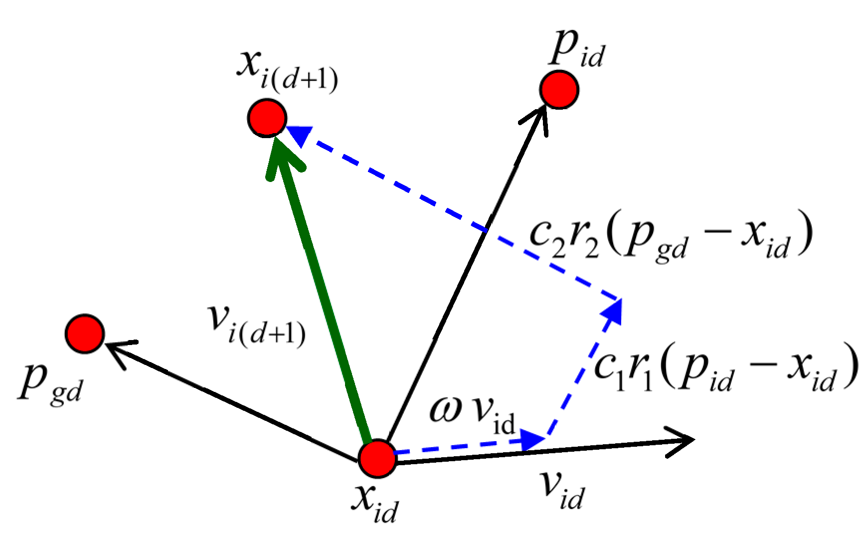
At starting period, the random population of swarms is generated with random position vectors and velocity of vectors X i = ( x i 1 , x i 2 , x i d ) and V i = ( v i 1 , v i 2 , v i d ) respectively. The best position of each particle is P i = ( p i 1 , p i 2 , p i d ) according to the best fitness value obtained by the particle time t . After iteration, the new positions and velocities to the particle for the next fitness evolution are calculated by the following equations [54]
v i d ( t + 1 ) = ω × v i d ( t ) + c 1 × φ 1 × ( p i d x i d ( t ) ) + c 1 × φ 2 × ( p g d x i d ( t ) )
x i d ( t + 1 ) = x i d ( t ) + v i d ( t + 1 )
where ω is inertia weight that plays a vital role to ensure the convergent behaviour of φ 1 and φ 2 which are uniform and random numbers with interval ( 0 , 1 ) . c 1 and c 2 are constants of acceleration, p i ( pbest ) is the personal best particle, and p g ( gbest ) is the best position of particle. The position of each parameter is illustrated in Figure 2.
The best position of the particle is the population so far [55]. The previous velocity can be represented by the first part of Equation (16). This equation provides the required momentum for the particles to roam across the search space. The second part of the Equation (16) is known as the “cognitive” part or component and it stands for the personal thinking of each particle. With the help of the cognitive component, the particles are encouraged to move toward their own best positions that are found. The third part of the Equation (16) is known as the “social” component to find the optimal global solution. The social component represents the effect of the collaboration of the particles. This part constantly drags the particles in the direction of the global best particle found so far.
A standard ACO has three control parameters, i.e., (i) the information heuristic factor, (ii) the expectation heuristic factor, and (iii) pheromone evaporation factor. In standard PSO, it also has three control parameters, i.e., (i) cognitive factor, (ii) social factors, and (iii) inertia weight. On the other hand, a standard ABC algorithm has only one control parameter, i.e., limit. In this paper, the expression for determining the value of limit is only depends on population (colony size) and the dimension of the problem (i.e. maximum cycle number). Apparently, these two common control parameters also exist in ACO and PSO. Therefore, ABC is the simplest algorithm among all.
There are several weaknesses of using meta-heuristic method such as ACO, PSO, and ABC. They tend to be trapped into local optima while doing the search. The process also requires long computational time with slow convergence speed. Although this method can find many parameters, it is difficult to encode the scheme. Despite these disadvantages, this method is capable of solving deterministic combinatorial problems, also combinatorial problems characterized by uncertainty [56,57].

4. Adaptive Neuro-Fuzzy Interface System

ANFIS system can be categorized to discrete control system by on-line identification, an approximation of a highly nonlinear function and it can predict a chaotic time series. The fuzzy “IF-THEN” rules, and predetermined inputs and outputs are used to construct for ANFIS system. The member functions (MFs) of ANFIS are created by input and output parameters. ANFIS obtains the FIS through the input, output, and algorithm of back propagation. FIS is executed by the combination of a database, a rule base, as well as the reasoning mechanism. Firstly, fuzzy logic finds the rule base. The database allocates the MFs that works in the rules of fuzzy logic. Finally, the reasoning mechanism reduces from the input data and rules which come to the feasible outcome. It can be adjusted to better performance for changing the environment. These systems have similar-human intelligence within a specific domain [58].
The ANFIS (training and evaluation) systems have been employed in the MATLAB. In ANFIS system, there are five input parameters to influence the power coefficient of the HAWT blade as shown in Table 1. The ‘IF-THEN’ rules of Takgi and Sugeno’s class of fuzzy logic with two inputs for the first order Sugeno are employed for the purpose of this study [59,60].
If x is P and y is R, then
f 1 = p 1 x + q 1 y + r 1
The input parameters of MFs that are made up of the 1st layer are providing the input values to the following layer. Each node is considered as an adaptive node having a node function 0 = μ P Q ( x ) and 0 = μ R S ( x ) , where μ P Q ( x ) and μ R S ( x ) are MFs. The maximum value of Triangle MFS is (1.0) and (0.0) is the minimum value. Like as,
μ ( x ) = t r i a n g l e ( x ; p i , q i , r i ) = { 0 , x p i x p i q i p i p i x p i r i x r i q i , q i x r i 0 , r i x }
where the set of parameters are { p i , q i , r i , } and x and y are the inputs to nodes and it signifies to tip speed ratio, blade radius, lift and drag ratio, solidity, chord length and the power coefficient.
In ANFIS system, the second layer of ANFIS is called a membership function. It looks for the weights of each function of membership. The first layer sends a signal to the membership function. The nodes of MFs are referred to as non-adaptive. The MFs layer refers to as a multiplier to receive to signal and send out the outcome in w i = μ P Q ( x ) × μ P Q ( y ) form. Output nodes are represented the firing strength of a rule.
The third layer is called a rule layer. In this layer, all the neurons perform as the pre-condition matching fuzzy rules. Every rule’s activation level is calculated by the several fuzzy rules which are equal to the number of layers. This layer’s node calculates the weights of normalized and it is considered as non-adaptive. Each node calculates the value of the rule’s firing strength over the sum of the rules firing strengths in the form of w i = w i w 1 w 2 , i = 1 , 2 . The results are mentioned to as the normalized firing strengths.
The 4th layer is known as the defuzzification layer. It is countable to provide the outcome values as the result of the inference of rules. Every node of the layer is an adaptive node having the following node function, 0 i 4 = w i x f = w i ( p i x + q i y + r i ) . Here, { p i , q i , r i } are the set of variable. This set variable is nominated as the consequent parameters.
0 i 5 = i w i x f = i w i f i w i
The final layer is called an output layer of ANFIS. The final layer obtains the inputs from the previous layer. After that, this layer is converted the fuzzy classification outputs into a binary (crisp) but this is not a non-adaptive layer. The structure of the ANFIS is shown in Figure 3. The total output is calculated by summing all signal received from the nodes.

5. Results and Discussion

5.1. Convergence Graph Power Coefficient and Computational Time

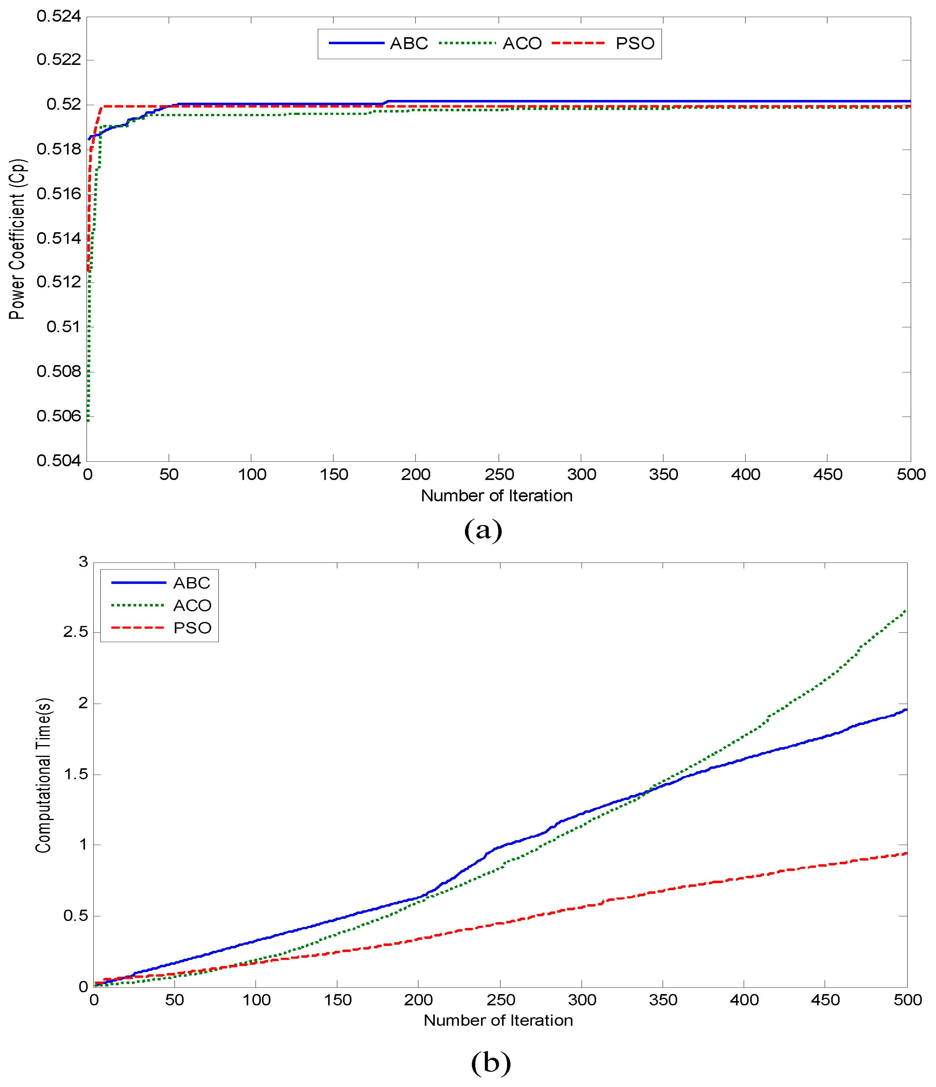
The convergence rate which is one of the key factors determines the reliability of an algorithm. It is usually considered as the higher the rate of convergence, the better the algorithm if only the outcomes converge and fall within the acceptable range. As discussed before, the nature-inspired algorithm produces the highest maximized objective function ( C p ) values from Equation (2) for every case, and thus, is directly ascertaining its accuracy. In this section, the manner of how fast the algorithm converges and attains its highest maximized value in the sequence of the number of iterations are investigated and discussed.
Figure 4a shows the convergence graph for all algorithms with 20 populations using ABC, ACO, and PSO algorithms. The maximum iteration has been varied from 100, 200, 300, 400, 500, and 600 iterations. It can be observed that the PSO has achieved a speedy convergence in the initial stage (achieved in less than 20 iterations). However, the searching for this algorithm tends to become stagnant after less than 10 iterations. When the search result comes at stagnant, all particles tend to assemble together around the global minimum, and thus, the global best result is not improved for time being. For ACO, it can be observed the search started at the lower value of power coefficient in comparison to ABC and PSO. However, the ants kept on searching the optimum value in less than around 350 iterations, which performed much better than the PSO, but became stagnant, or had no significant changes towards the end of the maximum iteration. For the ABC, the searching pattern shows the acceleration in convergence speed. For all cases, the convergence speed accelerated can be seen in less than around 200 iterations but became stagnant towards the end of the maximum iteration. It can be concluded that in terms of C p value, ABC has performed well in obtaining the highest value for all cases.
Computational time in Figure 4b refers to the time taken for the algorithm to finish from the first until the maximum number of iteration. The computation time of all algorithms is all in second (s). From Figure 4b, it can be observed that the PSO algorithm has taken ±1 s to finish the simulation for all cases. For the ABC algorithm, it needed around 2 s to finish the simulations. ACO needed more time than the ABC and PSO to complete the simulation, i.e., around 2.7 s.
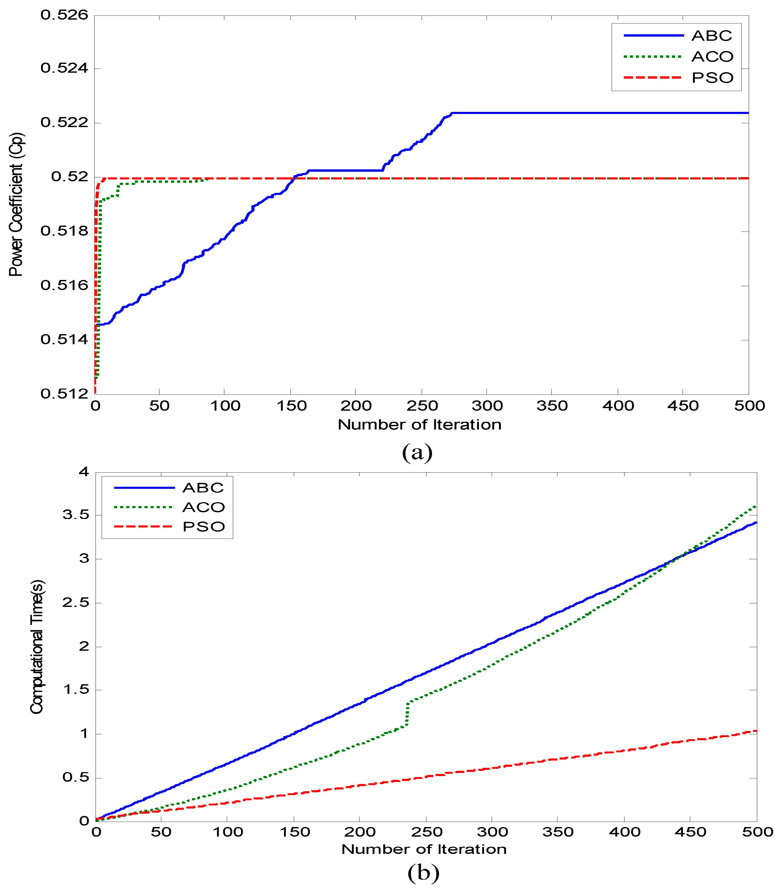
From Figure 5a, the convergence graphs are obtained with 50 populations for all algorithms with the iteration 100, 200, 300, 400, 500 and 600. PSO has achieved a speedy convergence in the initial stage but became stagnant from 10 iterations and onwards. For ACO, it can be noticed that the convergence graph of ACO is speedy after 50 iterations. After 50 iterations, ACO is not really improved until the maximum iteration. For ABC algorithms, the population kept on searching the optimum value in less than 250 iterations. With 50 populations, the C p obtained is almost similar to the result with 20 populations. The ABC algorithm has achieved the maximum power coefficient in comparison to PSO and ACO.
Figure 5b shows the computational time for 50 population’s size for all algorithms. The algorithm of ACO took the longest time, i.e., 3.6 s as compared to ABC and PSO. On the other hand, the PSO algorithm needed a much shorter time as compared to the ABC and ACO algorithms, which took around 0.6 s to complete the simulations.
Figure 6a shows the convergence progress for all algorithms with 100 populations. The maximum iteration varied from 100, 200, 300, 400, 500, and 600 iterations. It can be observed that the PSO achieved a speedy convergence in the initial stage (achieved in less than 50 iterations). For the ACO algorithm, it kept on searching for the optimum value within 100 iterations, and the result became stagnant after 250 iterations onwards. The final objective for PSO and ACO achieved an almost similar value. For ABC, the searching pattern shows an acceleration in the convergence speed. The acceleration in the convergence speed can be seen in less than 250 iterations. For ABC, it can be observed that the search started at the lower value of C p in comparison with ACO and PSO. In terms of C p value, the consistency of the ABC algorithm has been observed in comparison with ACO and PSO. It signifies that the ABC has outperformed PSO and ACO, with the highest maximize value of 0.5295 among all the compared algorithms ( ACO = 0.52   and   PSO = 0.52 ) .
From Figure 6b, PSO has completed the maximum iteration number in a shorter computational time, i.e., around 2.1 s in comparison to the ACO and ABC. The ABC algorithm has taken more time to complete the simulation compared to the ACO algorithm. It can be concluded that the computational time of all algorithms has taken within 6 s and it is acceptable and manageable for simulation purposes.

5.2. Prediction of Power Coefficient Using ANFIS

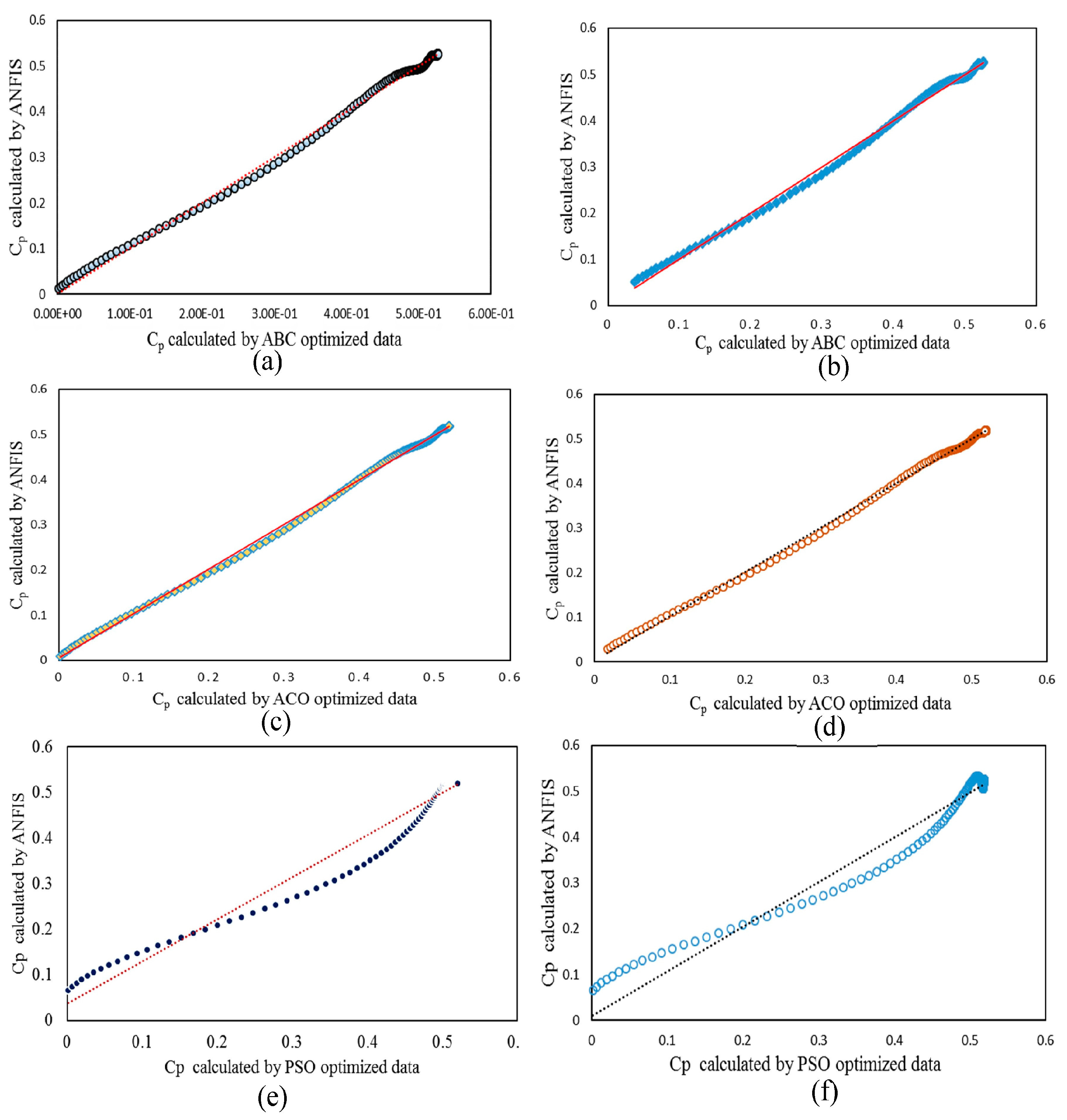
The best input combination of ABC, ACO, and PSO algorithms from Table 1 are used in ANFIS for the prediction of the power coefficient. To achieve the goal, 60% of the data is employed for training and 40% data is used for testing.
The scatter of Figure 7 showed the prediction of the power coefficient values via the ANFIS model against measured values of ABC optimization by Equation (2). Figure 7a provides the results for the training data set where it has been observed that most of the points drop along with the diagonal line. Figure 7b shows the testing data set where most of the points are very close to the diagonal line. From here, the predicted values via the ANFIS are very close to the measured values.
The predicted power coefficient training and testing values using ANFIS model for a wind turbine blade are presented in Figure 7c,d, respectively. These figures illustrate the training and testing values using the ANFIS model for a power coefficient and measured values of ACO optimization data. All values of data set for training and testing are very close to the diagonal line. Figure 7e,f show the training and testing data set of ANFIS, respectively. These data set of training and testing are measured from the best input combination of optimized values of PSO.
Most of the training and testing data are sometimes below the diagonal line and sometimes above the diagonal line. As seen in Table 2, the R2 correlation coefficients are near to 1. As a result, the proposed ANFIS model used for this investigation has a very good correlation with the power coefficient measured for training and testing data sets of three algorithms ABC, ACO, and PSO. Note that the R2 is higher for the ABC-ANFIS power coefficient as shown in Table 2 to compare ACO-ANFIS and PSO-ANFIS, which translates to a better correlation.
An ANFIS method is very helpful for the faster prediction of power coefficient with blade parameters. Figure 8 shows the wind power coefficient comparison between predicted and measured values by best input combination of ABC algorithm optimized parameters using ANFIS technique. From Figure 8, the measured (optimized) value ( C p = 0.5295 ) is very close to the predicted value, i.e., C p = 0.5215 with small variation.
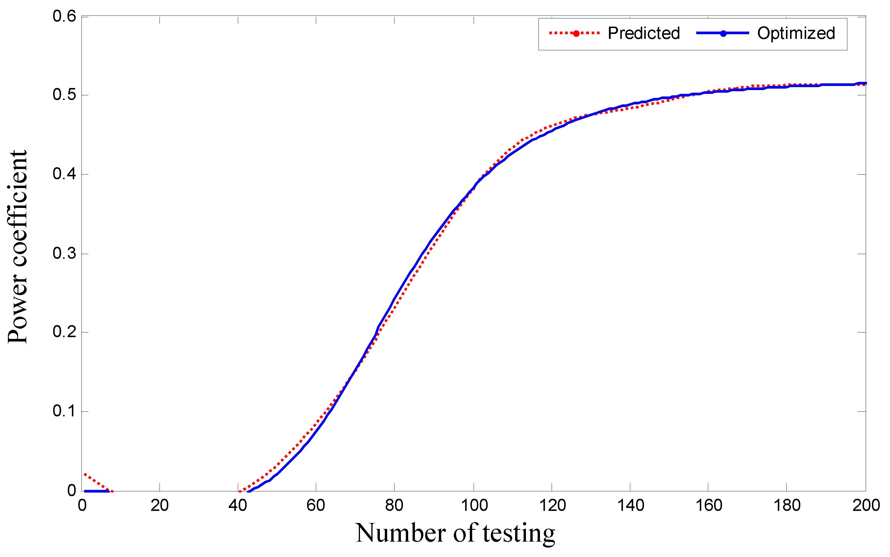
Figure 9 illustrates the predicted and optimized values of the ACO algorithm using ANFIS model for a power coefficient of the wind turbine blade. It can be observed that the predicted and measured values are almost similar whereas the predicted and optimized value is 0.5175 and 0.52, respectively.
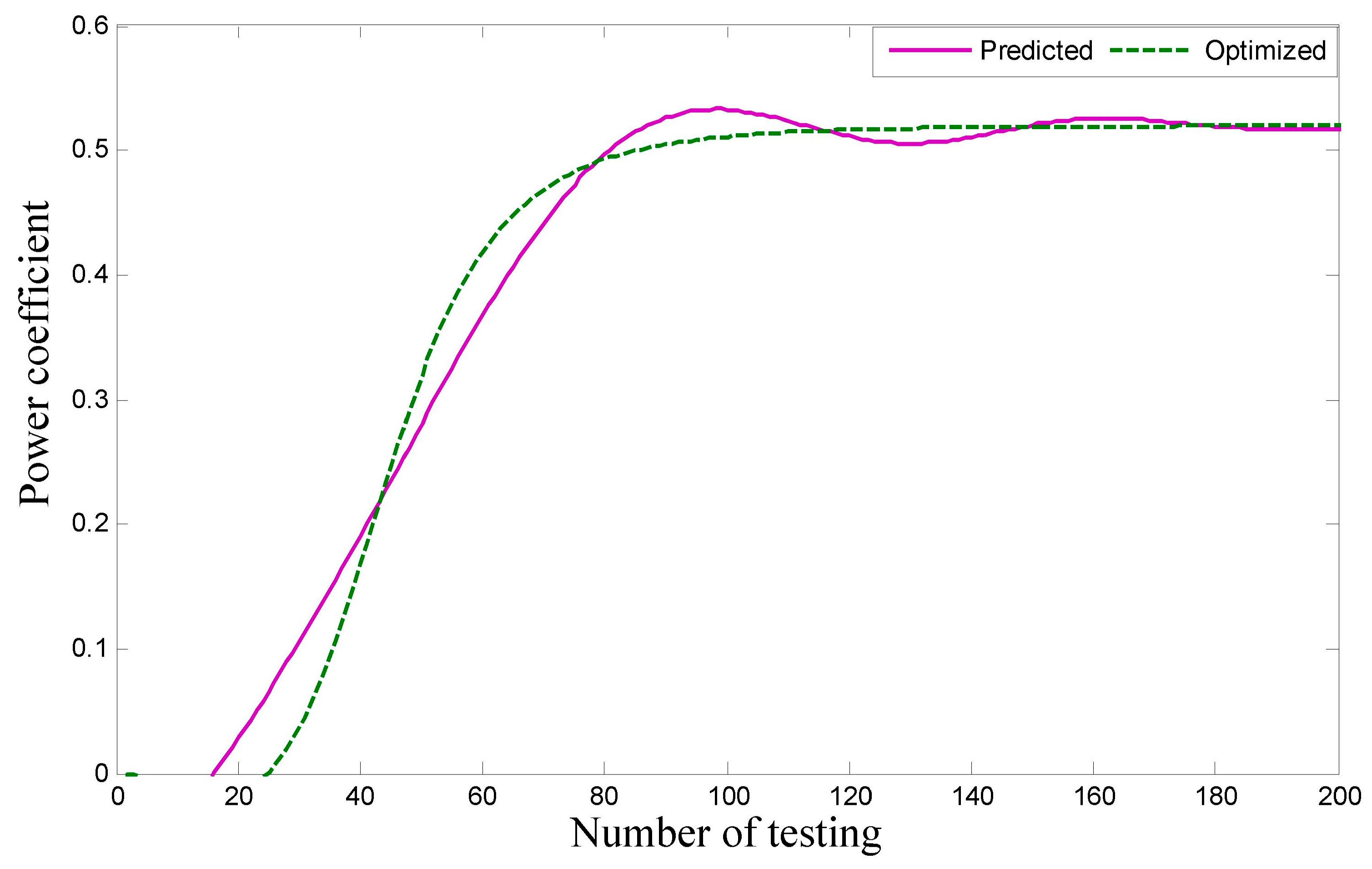
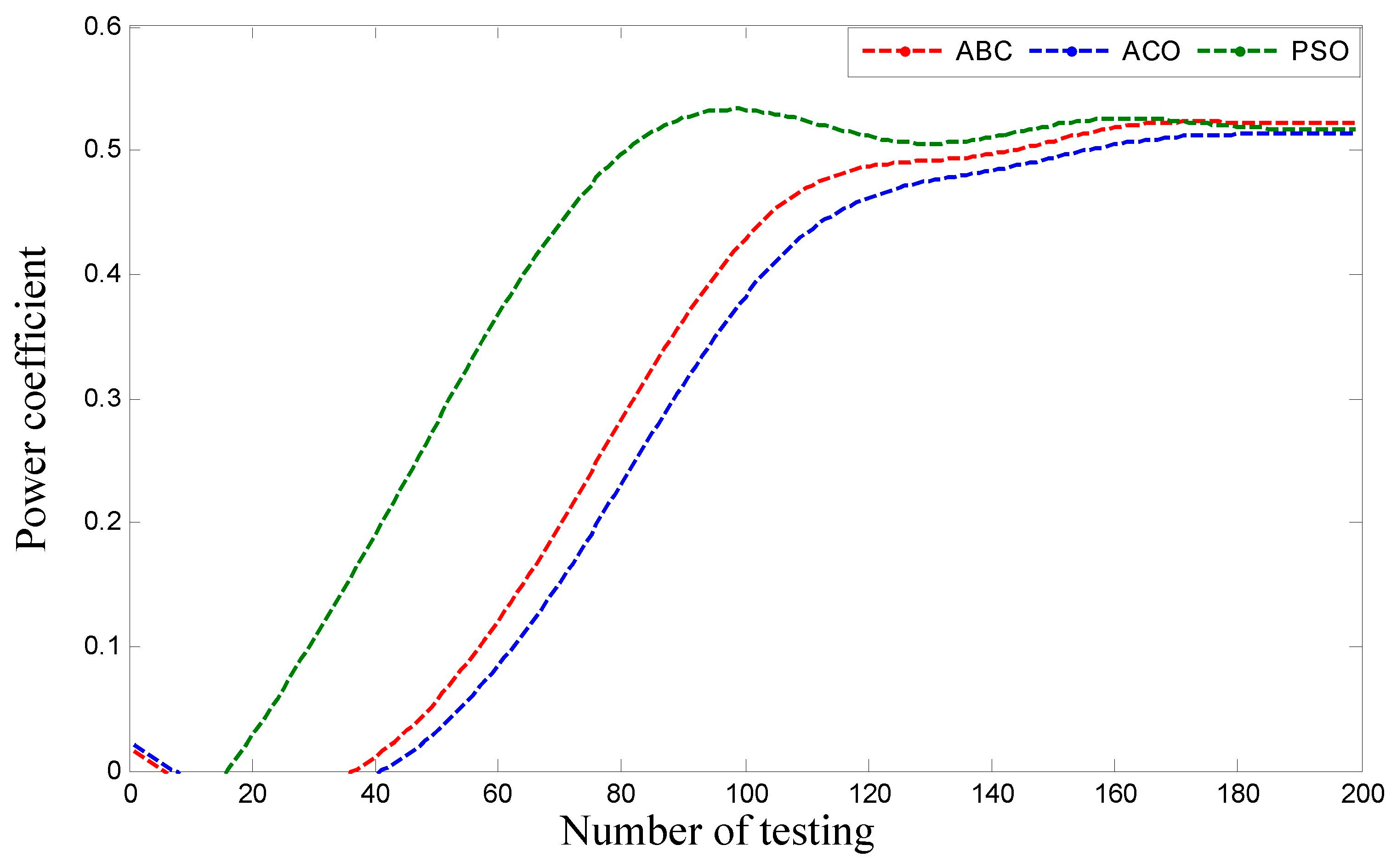
Figure 10 shows the predicted values 0.5135 and the measured values 0.52 of PSO algorithm for the power coefficient of wind turbine blades. Figure 11 shows the predicted power coefficient comparison between three algorithms (ABC, ACO, and PSO) values. The prediction of the power coefficient of the best input combination for getting the value of the ABC algorithm is higher compared to the ACO and PSO algorithms. Thus, the proposed ANFIS model has obtained high accuracy for predicting the wind turbine power coefficient of the three algorithms.
Table 2 approaches the results of the statistical analysis for the proposed ANFIS model for both training and testing values for ABC, ACO, and PSO. Several statistical indicators have been used to evaluate the proposed model performance, i.e., RMSE and R 2 as shown in Table 2. It should be noted that the units of RMSE and R 2 are dimensionless, respectively. Based on the results, the difference in RMSE and R 2 values for training and testing are relatively small. Therefore, it delivers additional evaluation and verification on the suitability of the proposed ANFIS model to estimate the power coefficient. The investigation results recommended that the proposed ANFIS model can effectively be implemented for prediction for all cases of ABC, ACO and PSO algorithms optimization. Based on the ANFIS results, the ABC algorithm shows better accuracy in both optimization and prediction as compared to ACO and PSO algorithm results. The ANFIS model has a very small RMSE (0.363) during testing and the value is slightly higher (0.00654) in training of the ABC-ANFIS model for the power coefficient. It has been observed that the ANFIS model showed constantly good correlation throughout the testing and training. It has been outperformed by ANFIS in terms of the effect on the wind turbine power coefficient. Therefore, the study results suggested that the proposed ANFIS model can effectively be embedded for the prediction of all cases of ABC, ACO, and PSO algorithm optimizations. Based on the ANFIS results, the ABC algorithms show better accuracy for both optimization and prediction compared to the ACO and PSO algorithms results.

5.3. Validation

Table 3 shows that the validation of this present investigation with related literatures. Sedaghat et al. [24] carried out the investigation of 300 kW horizontal axis wind turbine for aerodynamic design in the province of Semnan. They used the blade element momentum theory (BEM) for the blade “Airfoil is RISØ-A1-18”. The power coefficient was found to be 0.51 which was almost similar to our present investigation. Rajakumar et al. [5] optimized the power coefficient of the wind turbine rotor using the blade “Airfoil NACA 4410” and “NACA 2415” by CFD analysis. The power coefficients of the blade “Airfoil NACA 4410” and “NACA 2415” were found to be 0.48 and 0.45, respectively. The obtained power coefficients of both airfoils were slightly lower than the present investigation. Based on the supervisory control and data acquisition (SCADA) data, Dia et al. [63] investigated the power coefficient of wind turbines. The discovered power coefficient was 0.508, which was almost similar to our present investigation. Table 3 shows that the power coefficients of the present investigation are consistent and reliable with the findings of the other researchers. Therefore, it can be concluded that the power coefficient obtained from the literature supports our present study.

6. Conclusions

In conclusion, the blade design parameters have been obtained through optimization by nature-inspired algorithms (ABC, ACO, and PSO) with the objective function to maximize the C p . The prediction of power coefficient has also been carried out by using an ANFIS approach to satisfy the optimized results. The optimization process is employed on a non-linear maximization problem. ACO, PSO, and ABC have successfully been implemented to find the power coefficient for a wind turbine. The results have shown that ACO, PSO, and ABC have the ability to find the best combination of the five inputs of the HAWT blade parameters to get the optimum value of the power coefficient 0.520, 0.520, and 0.5295, respectively. It can be concluded that the ABC alogrithm has performed well to find the maximum value of the power coefficient compared to ACO and PSO.
It can be observed that the predicted values of the power coefficient for ABC = 0.5215 , ACO = 0.5175   and   PSO = 0.5135 are very close to the objective value ( C p ), i.e., ABC = 0.5295 , ACO = 0.52 , and   PSO = 0.52 . Therefore, it can be concluded that the presented prediction (ABC-ANFIS, ACO-ANFIS and PSO-ANFIS) are acceptable based on the RMSE and R 2 . The values of R2 are near to value 1 which are suitable for the better prediction results. Based on the ANFIS results, the effectiveness of ABC algorithm is more accurate for both optimization and prediction in comparison to ACO and PSO algorithms. By using ANFIS, it can be used for more complex problem solutions, such as accuracy, identification, and prediction of the power coefficient of the HAWT blades. The results have been obtained by optimization and prediction results and can be used for further design and prototype horizontal axis wind turbine modeling. The comparison with similar literature for the power coefficient also shows the consistent results, which supports our present investigation.

Author Contributions

All authors discussed and agreed on the idea and contribution. M.R.S. contributed to the writing manuscript, mathematical modeling, simulation, and prediction. S.J. contributed to optimizing the model and simulation. S.J., C.W.T., and S.F.T. contributed to the revisions and discussion of the results.

Funding

This research was funded by Ministry of Higher Education of Malaysia and University Malaya (ERGS No. ER0142013A and High Impact Research Grant (HIR-D000006-16001)).

Acknowledgments

The authors would like to express their gratitude to the Ministry of Higher Education of Malaysia and University Malaya (ERGS No. ER0142013A and High Impact Research Grant (HIR-D000006-16001)) for funding and providing facilities to conduct the research.

Conflicts of Interest

The authors declare no conflict of interest.

References

  1. Eltamaly, A.M.; Farh, H.M. Maximum power extraction from wind energy system based on fuzzy logic control. Electr. Power Syst. Res. 2013, 97, 144–150. [Google Scholar] [CrossRef]
  2. Oghafy, V.; Nikkhajoei, H. Maximum power extraction for a wind-turbine generator with no wind speed sensor. In Proceedings of the 2008 IEEE Power and Energy Society General Meeting-Conversion and Delivery of Electrical Energy in the 21st Century, Pittsburgh, PA, USA, 20–24 July 2008; pp. 1–6. [Google Scholar]
  3. Marques, J.; Pinheiro, H.; Gründling, H.; Pinheiro, J.; Hey, H. A survey on variable-speed wind turbine system. Network 2003, 24, 26. [Google Scholar]
  4. Lanzafame, R.; Messina, M. Horizontal axis wind turbine working at maximum power coefficient continuously. Renew. Energy 2010, 35, 301–306. [Google Scholar] [CrossRef]
  5. Rajakumar, S.; Ravindran, D. Iterative approach for optimising coefficient of power, coefficient of lift and drag of wind turbine rotor. Renew. Energy 2012, 38, 83–93. [Google Scholar] [CrossRef]
  6. Petković, D.; Ćojbašić, Ž.; Nikolić, V.; Shamshirband, S.; Kiah, M.L.M.; Anuar, N.B.; Wahab, A.W.A. Adaptive neuro-fuzzy maximal power extraction of wind turbine with continuously variable transmission. Energy 2014, 64, 868–874. [Google Scholar] [CrossRef]
  7. Eroğlu, Y.; Seçkiner, S.U. Design of wind farm layout using ant colony algorithm. Renew. Energy 2012, 44, 53–62. [Google Scholar] [CrossRef]
  8. Fuchs, I.; Gjengedal, T. Ant colony optimization and analysis of time step resolution in transmission expansion computations for wind power integration. In Proceedings of the 2011 16th International Conference on Intelligent System Application to Power Systems (ISAP2011), Hersonissos, Greece, 25–28 September 2011; pp. 1–6. [Google Scholar]
  9. Jovanovic, R.; Tuba, M.; Voß, S. An ant colony optimization algorithm for partitioning graphs with supply and demand. Appl. Soft Comput. 2016, 41, 317–330. [Google Scholar] [CrossRef] [Green Version]
  10. Abd-Allah, M.; Said, A.; Ali, M.N. Mitigation of lightning hazards at the more sensitive points in wind farms using ant-colony optimization technique. Int. Electr. Eng. J. 2015, 6, 1856–1868. [Google Scholar]
  11. Mustafar, M.F.; Musirin, I.; Kalil, M.R.; Idris, M.K. Ant colony optimization (aco) based technique for voltage control and loss minimization using transformer tap setting. In Proceedings of the 2007 5th Student Conference on Research and Development (SCOReD 2007), Selangor, Malaysia, 11–12 December 2007; pp. 1–6. [Google Scholar]
  12. Delgarm, N.; Sajadi, B.; Delgarm, S. Multi-objective optimization of building energy performance and indoor thermal comfort: A new method using artificial bee colony (ABC). Energy Build. 2016, 131, 42–53. [Google Scholar] [CrossRef]
  13. Song, J.; Romero, C.E.; Yao, Z.; He, B. Improved artificial bee colony-based optimization of boiler combustion considering NOX emissions, heat rate and fly ash recycling for on-line applications. Fuel 2016, 172, 20–28. [Google Scholar] [CrossRef]
  14. Ebrahim, E.A. Artificial Bee Colony-Based Design of Optimal On-Line Self-tuning PIDController Fed AC Drives. Int. J. Eng. Res. 2014, 3, 807–811. [Google Scholar]
  15. Derakhshan, S.; Tavaziani, A.; Kasaeian, N. Numerical shape optimization of a wind turbine blades using artificial bee colony algorithm. J. Energy Resour. Technol. 2015, 137, 051210. [Google Scholar] [CrossRef]
  16. Habbi, H.; Boudouaoui, Y.; Karaboga, D.; Ozturk, C. Self-generated fuzzy systems design using artificial bee colony optimization. Inf. Sci. 2015, 295, 145–159. [Google Scholar] [CrossRef]
  17. Safaei, A.; Vahidi, B.; Askarian-Abyaneh, H.; Azad-Farsani, E.; Ahadi, S. A two step optimization algorithm for wind turbine generator placement considering maximum allowable capacity. Renew. Energy 2016, 92, 75–82. [Google Scholar] [CrossRef]
  18. Wan, C.; Wang, J.; Yang, G.; Zhang, X. Optimal micro-siting of wind farms by particle swarm optimization. In Proceedings of the International Conference in Swarm Intelligence, Beijing, China, 12–15 June 2010; pp. 198–205. [Google Scholar]
  19. Pookpunt, S.; Ongsakul, W. Optimal placement of wind turbines within wind farm using binary particle swarm optimization with time-varying acceleration coefficients. Renew. Energy 2013, 55, 266–276. [Google Scholar] [CrossRef]
  20. Maleki, A.; Ameri, M.; Keynia, F. Scrutiny of multifarious particle swarm optimization for finding the optimal size of a PV/wind/battery hybrid system. Renew. Energy 2015, 80, 552–563. [Google Scholar] [CrossRef]
  21. Jang, J.-S.R. ANFIS: Adaptive-network-based fuzzy inference system. IEEE Trans. Syst. Man Cybern. 1993, 23, 665–685. [Google Scholar] [CrossRef]
  22. Petković, D.; Ćojbašič, Ž.; Nikolić, V. Adaptive neuro-fuzzy approach for wind turbine power coefficient estimation. Renew. Sustain. Energy Rev. 2013, 28, 191–195. [Google Scholar] [CrossRef]
  23. Shamshirband, S.; Petković, D.; Saboohi, H.; Anuar, N.B.; Inayat, I.; Akib, S.; Ćojbašić, Ž.; Nikolić, V.; Kiah, M.L.M.; Gani, A. Wind turbine power coefficient estimation by soft computing methodologies: Comparative study. Energy Convers. Manag. 2014, 81, 520–526. [Google Scholar] [CrossRef]
  24. Sedaghat, A.; Mirhosseini, M. Aerodynamic design of a 300kW horizontal axis wind turbine for province of Semnan. Energy Convers. Manag. 2012, 63, 87–94. [Google Scholar] [CrossRef]
  25. Rajakumar, S.; Durairaj, R.; Kumar, M.; Venkatachalam, G.; Muthukumar, S. Optimization of power coefficient of wind turbine using genetic algorithm. J. Inst. Eng. (India) 2017, 98, 111–118. [Google Scholar] [CrossRef]
  26. Arifujjaman, M. Modeling and optimization of power coefficient using 2K factorial methodology. In Proceedings of the 2010 IEEE Electrical Power & Energy Conference, Halifax, NS, Canada, 25–27 August 2010; pp. 1–6. [Google Scholar]
  27. Selig, M.S.; Coverstone-Carroll, V.L. Application of a genetic algorithm to wind turbine design. J. Energy Resour. Technol. 1996, 118, 22–28. [Google Scholar] [CrossRef]
  28. Jureczko, M.; Pawlak, M.; Mężyk, A. Optimisation of wind turbine blades. J. Mater. Process. Technol. 2005, 167, 463–471. [Google Scholar] [CrossRef]
  29. Khalfallah, M.G.; Koliub, A.M. Suggestions for improving wind turbines power curves. Desalination 2007, 209, 221–229. [Google Scholar] [CrossRef]
  30. Sayed, M.A.; Kandil, H.A.; Shaltot, A. Aerodynamic analysis of different wind-turbine-blade profiles using finite-volume method. Energy Convers. Manag. 2012, 64, 541–550. [Google Scholar] [CrossRef]
  31. Manwell, J.F.; McGowan, J.G.; Rogers, A.L. Wind Energy Explained: Theory, Design and Application; John Wiley & Sons: West Sussex, UK, 2010. [Google Scholar]
  32. Zhu, J.; Cai, X.; Gu, R. Aerodynamic and Structural Integrated Optimization Design of Horizontal-Axis Wind Turbine Blades. Energies 2016, 9, 66. [Google Scholar] [CrossRef]
  33. Kim, B.; Kim, W.; Lee, S.; Bae, S.; Lee, Y. Developement and verification of a performance based optimal design software for wind turbine blades. Renew. Energy 2013, 54, 166–172. [Google Scholar] [CrossRef]
  34. Burton, T.; Jenkins, N.; Sharpe, D.; Bossanyi, E. Aerodynamics of horizontal axis wind turbines. In Wind Energy Handbook, 2nd ed.; John Wiley & Sons: West Sussex, UK, 2011. [Google Scholar]
  35. Bai, C.-J.; Chen, P.-W.; Wang, W.-C. Aerodynamic design and analysis of a 10 kW horizontal-axis wind turbine for Tainan, Taiwan. Clean Technol. Environ. Policy 2016, 18, 1151–1166. [Google Scholar] [CrossRef]
  36. Singh, M.; Chandra, A. Application of adaptive network-based fuzzy inference system for sensorless control of PMSG-based wind turbine with nonlinear-load-compensation capabilities. IEEE Trans. Power Electron. 2011, 26, 165–175. [Google Scholar] [CrossRef]
  37. Dorigo, M.; Gambardella, L.M. Ant colonies for the travelling salesman problem. BioSystems 1997, 43, 73–81. [Google Scholar] [CrossRef] [Green Version]
  38. Shen, Q.; Jiang, J.-H.; Tao, J.-C.; Shen, G.-L.; Yu, R.-Q. Modified ant colony optimization algorithm for variable selection in QSAR modeling: QSAR studies of cyclooxygenase inhibitors. J. Chem. Inf. Model. 2005, 45, 1024–1029. [Google Scholar] [CrossRef] [PubMed]
  39. Dorigo, M.; Birattari, M.; Stützle, T. Ant colony optimization. IEEE Comput. Intell. Mag. 2006, 1, 28–39. [Google Scholar] [CrossRef]
  40. Socha, K.; Dorigo, M. Ant colony optimization for continuous domains. Eur. J. Oper. Res. 2008, 185, 1155–1173. [Google Scholar] [CrossRef] [Green Version]
  41. Kıran, M.S.; Özceylan, E.; Gündüz, M.; Paksoy, T. A novel hybrid approach based on particle swarm optimization and ant colony algorithm to forecast energy demand of Turkey. Energy Convers. Manag. 2012, 53, 75–83. [Google Scholar] [CrossRef]
  42. Galdi, V.; Piccolo, A.; Siano, P. Designing an adaptive fuzzy controller for maximum wind energy extraction. IEEE Trans. Energy Convers. 2008, 23, 559–569. [Google Scholar] [CrossRef]
  43. Karaboga, D. An Idea Based on Honey Bee Swarm for Numerical Optimization; Technical Report-TR06; Erciyes University, Engineering Faculty, Computer Engineering Department: Kayseri, Turkey, 2005. [Google Scholar]
  44. Karaboga, D.; Basturk, B. A powerful and efficient algorithm for numerical function optimization: Artificial bee colony (ABC) algorithm. J. Glob. Optim. 2007, 39, 459–471. [Google Scholar] [CrossRef]
  45. Singh, S.; Kaushik, S.C. Optimal sizing of grid integrated hybrid PV-biomass energy system using artificial bee colony algorithm. IET Renew. Power Gener. 2016, 10, 642–650. [Google Scholar] [CrossRef]
  46. Akay, B.; Karaboga, D. A modified artificial bee colony algorithm for real-parameter optimization. Inf. Sci. 2012, 192, 120–142. [Google Scholar] [CrossRef]
  47. Karaboga, D.; Akay, B. A modified artificial bee colony (ABC) algorithm for constrained optimization problems. Appl. Soft Comput. 2011, 11, 3021–3031. [Google Scholar] [CrossRef]
  48. Song, X.; Gu, H.; Tang, L.; Zhao, S.; Zhang, X.; Li, L.; Huang, J. Application of artificial bee colony algorithm on surface wave data. Comput. Geosci. 2015, 83, 219–230. [Google Scholar] [CrossRef]
  49. Dufo-López, R.; Bernal-Agustín, J.L.; Contreras, J. Optimization of control strategies for stand-alone renewable energy systems with hydrogen storage. Renew. Energy 2007, 32, 1102–1126. [Google Scholar] [CrossRef]
  50. Bai, Q. Analysis of particle swarm optimization algorithm. Comput. Inf. Sci. 2010, 3, 180. [Google Scholar] [CrossRef]
  51. Kennedy, J.; Kennedy, J.F.; Eberhart, R.C.; Shi, Y. Swarm Intelligence; Morgan Kaufmann: Burlington, MA, USA, 2001. [Google Scholar]
  52. Eberhart, R.C.; Kennedy, J. A new optimizer using particle swarm theory. In Proceedings of the Sixth International Symposium on Micro Machine and Human Science, Nagoya, Japan, 4–6 October 1995; pp. 39–43. [Google Scholar]
  53. Eberhart, R.C.; Shi, Y. Comparing inertia weights and constriction factors in particle swarm optimization. In Proceedings of the 2000 Congress on Evolutionary Computation, La Jolla, CA, USA, 16–19 July 2000; pp. 84–88. [Google Scholar]
  54. Shi, Y.; Eberhart, R. A modified particle swarm optimizer. In Proceedings of the 1998 IEEE International Conference on Evolutionary Computation Proceedings. IEEE World Congress on Computational Intelligence, Anchorage, AK, USA, 4–9 May 1998; pp. 69–73. [Google Scholar]
  55. Shi, Y.; Eberhart, R.C. Parameter selection in particle swarm optimization. In Proceedings of the International Conference on Evolutionary Programming, San Diego, CA, USA, 24–27 March 1998; pp. 591–600. [Google Scholar]
  56. Eberhart, R.C.; Shi, Y.; Kennedy, J. Swarm Intelligence (Morgan Kaufmann Series in Evolutionary Computation); Morgan Kaufmann: Burlington, MA, USA, 2001. [Google Scholar]
  57. Dilmac, S.; Nizam, A.; Korurek, M. Evaluation of a new heart beat classification method based on ABC algorithm, comparison with GA, PSO and ACO classifiers. Int. J. Reason.-Based Intell. Syst. 2014, 6, 98–108. [Google Scholar] [CrossRef]
  58. Petković, D.; Shamshirband, S. Soft methodology selection of wind turbine parameters to large affect wind energy conversion. Int. J. Electr. Power Energy Syst. 2015, 69, 98–103. [Google Scholar] [CrossRef]
  59. Mamdani, E.H.; Assilian, S. An experiment in linguistic synthesis with a fuzzy logic controller. Int. J. Man-Mach. Stud. 1975, 7, 1–13. [Google Scholar] [CrossRef]
  60. Al-Hmouz, A.; Shen, J.; Al-Hmouz, R.; Yan, J. Modeling and simulation of an Adaptive Neuro-Fuzzy Inference System (ANFIS) for mobile learning. IEEE Trans. Learn. Technol. 2012, 5, 226–237. [Google Scholar] [CrossRef]
  61. Tangler, J.L.; Somers, D.M. NREL Airfoil Families for HAWTs; Citeseer: Golden, CO, USA, 1995. [Google Scholar]
  62. Giguere, P.; Selig, M.S. Low Reynolds number airfoils for small horizontal axis wind turbines. Wind Eng. 1997, 21, 367–380. [Google Scholar]
  63. Dai, J.; Liu, D.; Wen, L.; Long, X. Research on power coefficient of wind turbines based on SCADA data. Renew. Energy 2016, 86, 206–215. [Google Scholar] [CrossRef]
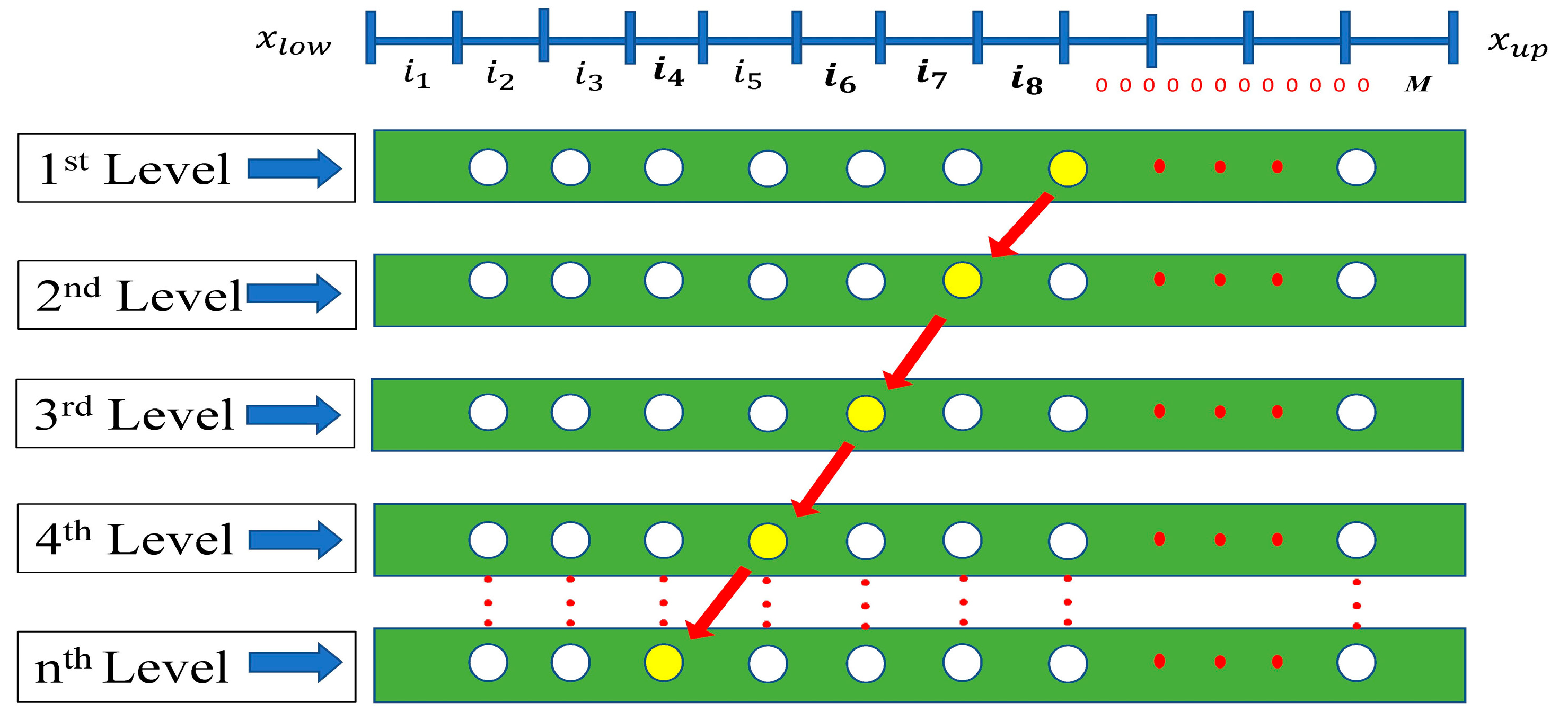
Figure 1. State space graph of ACO.
Symmetry 11 00456 g001
Figure 2. Particle swarm optimization algorithm.
Symmetry 11 00456 g002
Figure 3. The structure of ANFIS.
Symmetry 11 00456 g003
Figure 4. (a) Convergence graph; (b) computational time of ABC, ACO, and PSO with 20 populations.
Symmetry 11 00456 g004
Figure 5. (a) Convergence graph; (b) computational time of ABC, ACO, and PSO with 50 populations.
Symmetry 11 00456 g005
Figure 6. (a) Convergence graph; (b) computational time of ABC, ACO, and PSO with 100 populations.
Symmetry 11 00456 g006
Figure 7. Training and testing data: (a) training data set of ABC; (b) testing data set of ABC; (c) training data set of ACO; (d) testing data set of ACO; (e) training data set of PSO, and (f) testing data set of PSO.
Symmetry 11 00456 g007
Figure 8. Predicted (ANFIS) vs. optimized (ABC) of the power coefficient (Cp).
Symmetry 11 00456 g008
Figure 9. Predicted (ANFIS) vs. optimized (ACO) of the power coefficient (Cp).
Symmetry 11 00456 g009
Figure 10. Predicted (ANFIS) vs. optimized (PSO) of the power coefficient (Cp).
Symmetry 11 00456 g010
Figure 11. Prediction of ABC, ACO, and PSO.
Symmetry 11 00456 g011
Table 1. The best input combination for optimum values power coefficient using ABC, ACO, and PSO.
Input/output ParametersInput VariablesABCACOPSO
Tip Speed Ratio3 to 10 [24]6.44796.00326.00
Blade Radius1 to 5 [61]4.0164.30894.50
Lift to drag ratio1 to 110 [61]109.4848109.9935110.00
Solidity ratio0.01 to 0.45 [35]0.38850.350.45
Chord length0.01 to 0.45 [62]0.1930.2320.40
Power coefficient 0.5290.520.52
Table 2. Performance of the established training and testing of the ANFIS models for the power coefficient based on statistical indicators.
ModelTrainingTesting
RMSE ( W / m 2 ) R 2 RMSE ( W / m 2 ) R 2
ABC-ANFIS0.006540.9990.3630.9985
ACO-ANFIS0.005440.99890.8140.997
PSO-ANFIS0.2350.97111.9110.9777
Table 3. Validation of this present investigation with related literature.
SubjectTheoryBlade ModelMaximum CP
Present InvestigationABC algorithmsAirfoil S8220.529
ACO algorithms0.52
PSO algorithms0.52
ABC-ANFIS0.5215
ACO-ANFIS0.5175
PSO0-ANFIS0.5135
ValidationBlade element momentum theory (BEM) [24]Airfoil is RISØ-A1-180.51
CFD analysis [5]NACA 44100.48
NACA 24150.45
Supervisory control and data acquisition (SCADA) system [63]----------0.508