Abstract
In this paper, we solve a long-standing open problem in the field of fuzzy logics, that is, the standard completeness for the involutive uninorm logic IUL. In fact, we present a uniform method of density elimination for several semilinear substructural logics. Especially, the density elimination for IUL is proved. Then the standard completeness for IUL follows as a lemma by virtue of previous work by Metcalfe and Montagna.
Keywords:
density elimination; involutive uninorm logic; standard completeness of HpsUL *; semilinear substructural logics; fuzzy logic MSC:
03B50; 03F05; 03B52; 03B47
1. Introduction
The problem of the completeness of Łukasiewicz infinite-valued logic (Ł, for short) was posed by Łukasiewicz and Tarski in the 1930s. It was twenty-eight years later that it was syntactically solved by Rose and Rosser [1]. Chang [2] developed at almost the same time a theory of algebraic systems for Ł, which are called MV-algebras, with an attempt to make MV-algebras correspond to Ł as Boolean algebras to the classical two-valued logic. Chang [3] subsequently finished another proof for the completeness of Ł by virtue of his MV-algebras.
It was Chang who observed that the key role in the structure theory of MV-algebras is not locally finite MV-algebras but linearly ordered ones. The observation was formalized by Hájek [4] who showed the completeness for his basic fuzzy logic (BL for short) with respect to linearly ordered BL-algebras. Starting with the structure of BL-algebras, Hájek [5] reduced the problem of the standard completeness of BL to two formulas to be provable in BL. Here and thereafter, by the standard completeness we mean that logics are complete with respect to algebras with lattice reduct [0, 1]. Cignoli et al. [6] subsequently proved the standard completeness of BL, i.e., BL is the logic of continuous t-norms and their residua.
Hajek’s approach toward fuzzy logic has been extended by Esteva and Godo in [7], where the authors introduced the logic MTL which aims at capturing the tautologies of left-continuous t-norms and their residua. The standard completeness of MTL was proved by Jenei and Montagna in [8], where the major step is to embed linearly ordered MTL-algebras into the dense ones under the situation that the structure of MTL-algebras have been unknown as of yet.
Esteva and Godo’s work was further promoted by Metcalfe and Montagna [9] who introduced the uninorm logic UL and involutive uninorm logic (IUL) which aims at capturing tautologies of left-continuous uninorms and their residua and those of involutive left-continuous ones, respectively. Recently, Cintula and Noguera [10] introduced semilinear substructural logics which are substructural logics complete with respect to linearly ordered models. Almost all well-known families of fuzzy logics such as Ł, BL, MTL, UL and IUL belong to the class of semilinear substructural logics.
Metcalfe and Montagna’s method to prove standard completeness for UL and its extensions is of proof theory in nature and consists of two key steps. Firstly, they extended UL with the density rule of Takeuti and Titani [11]:
where p does not occur in or C, and then prove the logics with are complete with respect to algebras with lattice reduct [0, 1]. Secondly, they give a syntactic elimination of that was formulated as a rule of the corresponding hypersequent calculus.
Hypersequents are a natural generalization of sequents which were introduced independently by Avron [12] and Pottinger [13] and have proved to be particularly suitable for logics with prelinearity [9,14]. Following the spirit of Gentzen’s cut elimination, Metcalfe and Montagna succeeded to eliminate the density rule for GUL and several extensions of GUL by induction on the height of a derivation of the premise and shifting applications of the rule upwards, but failed for GIUL and therefore left it as an open problem.
There are several relevant works about the standard completeness of IUL as follows. With an attempt to prove the standard completeness of IUL, we generalized Jenei and Montagna’s method [15] for IMTL in [16], but our effort was only partially successful. It seems that the subtle reason why it does not work for UL and IUL is the failure of the finite model property of these systems [17]. Jenei [18] constructed several classes of involutive FL-algebras, as he said, in order to gain a better insight into the algebraic semantic of the substructural logic IUL, and also to the long-standing open problem about its standard completeness. Ciabattoni and Metcalfe [19] introduced the method of density elimination by substitutions which is applicable to a general class of (first-order) hypersequent calculi but fails in the case of GIUL.
We reconsidered Metcalfe and Montagna’s proof-theoretic method to investigate the standard completeness of IUL, because they have proved the standard completeness of UL by their method and we cannot prove such a result by the Jenei and Montagna’s model-theoretic method. In order to prove the density elimination for GUL, they prove that the following generalized density rule :
is admissible for GUL, where they set two constraints to the form of : (i) and for some ; (ii) p does not occur in , , , for , , .
We may regard as a procedure whose input and output are the premise and conclusion of , respectively. We denote the conclusion of by when its premise is . Observe that Metcalfe and Montagna had succeeded in defining the suitable conclusion for an almost arbitrary premise in , but it seems impossible for GIUL (see Section 3 for an example). We then define the following generalized density rule for
and prove its admissibility in Section 9.
Theorem 1 (Main theorem).
Let , p does not occur in or for all ,. Then the strong density rule
is admissible in .
In proving the admissibility of , Metcalfe and Montagna made some restriction on the proof of , i.e., converted into an r-proof. The reason why they need an r-proof is that they set the constraint (i) to . We may imagine the restriction on and the constraints to as two pallets of a balance, i.e., one is strong if another is weak and vice versa. Observe that we select the weakest form of in that guarantees the validity of . Then it is natural that we need make the strongest restriction on the proof of . But it seems extremely difficult to follow such a way to prove the admissibility of .
In order to overcome such a difficulty, we first of all choose Avron-style hypersequent calculi as the underlying systems (see Appendix A.1). Let be a cut-free proof of in . Starting with , we construct a proof of in a restricted subsystem of by a systematic novel manipulations in Section 4. Roughly speaking, each sequent of G is a copy of some sequent of , and each sequent of is a copy of some contraction sequent in . In Section 5, we define the generalized density rule in and prove that it is admissible.
Now, starting with and its proof , we construct a proof of in such that each sequent of is a copy of some sequent of G. Then by the admissibility of . Then by Lemma 29. Hence the density elimination theorem holds in . Especially, the standard completeness of IUL follows from Theorem 62 of [9].
is constructed by eliminating -sequents in one by one. In order to control the process, we introduce the set of -nodes of and the set of the branches relative to I and construct such that does not contain -sequents lower than any node in I, i.e., implies for all . The procedure is called the separation algorithm of branches in which we introduce another novel manipulation and call it derivation-grafting operation in Section 7 and Section 8.
2. Preliminaries
In this section, we recall the basic definitions and results involved, which are mainly from [9]. Substructural fuzzy logics are based on a countable propositional language with formulas built inductively as usual from a set of propositional variables VAR, binary connectives and constants with definable connective
Definition 1.
([9,12]) A sequent is an ordered pair of finite multisets (possibly empty) of formulas, which we denote by . Γ and Δ are called the antecedent and succedents, respectively, of the sequent and each formula in Γ and Δ is called a sequent-formula. A hypersequent G is a finite multiset of the form , where each is a sequent and is called a component of G for each . If contains at most one formula for , then the hypersequent is single-conclusion, otherwise it is a multiple-conclusion.
Definition 2.
Let S be a sequent and a hypersequent. We say that if S is one of .
Notation 1.
Let and be two hypersequents. We will assume from now on that all set terminology refers to multisets, adopting the conventions of writing for the multiset union of Γ and Δ, A for the singleton multiset , and for the multiset union of λ copies of Γ for . By we mean that for all and the multiplicity of S in is not more than that of S in . We will use , , , by their standard meaning for multisets by default and we will declare when we use them for sets. We sometimes write and as , (or ), respectively.
Definition 3.
([12]) A hypersequent rule is an ordered pair consisting of a sequence of hypersequents called the premises (upper hypersequents) of the rule, and a hypersequent G called the conclusion (lower hypersequent), written by If , then the rule has no premise and is called an initial sequent. The single-conclusion version of a rule adds the restriction that both the premises and conclusion must be single-conclusion; otherwise the rule is multiple-conclusion.
Definition 4.
([9])GULandGIULconsist of the single-conclusion and multiple-conclusion versions of the following initial sequents and rules, respectively:
Initial sequents
Structural rules
Logical rules
Cut rule
Definition 5.
([9])GMTLandGIMTLareGULandGIULplus the single conclusion and multiple-conclusion versions, respectively, of:
Definition 6.
(i) and
;
(ii) By (or we denote an instance of a two-premise rule (or one-premise rule ) of , where and are its focus sequents and is its principle sequent (for , , and or hypersequent (for , and , see Definition 12).
Definition 7.
([9]) is extended with the following density rule:
where p does not occur in or .
Definition 8.
([12]) A derivation τ of a hypersequent G from hypersequents in a hypersequent calculus is a labeled tree with the root labeled by G, leaves labeled initial sequents or some , and for each node labeled with parent nodes labeled (where possibly , is an instance of a rule of .
Notation 2.
(i) denotes that τ is a derivation of from ;
(ii) Let H be a hypersequent. denotes that H is a node of τ. We call H a leaf hypersequent if H is a leaf of τ, the root hypersequent if it is the root of τ. denotes that and its parent nodes are ;
(iii) Let then denotes the subtree of τ rooted at H;
(iv) τ determines a partial order with the root as the least element. denotes and for any . By we mean that is the same node as in τ. We sometimes write as ⩽;
(v) An inference of the form is called the full external contraction and denoted by , if , is not a lower hypersequent of an application of whose contraction sequent is S, and not an upper one in τ.
Definition 9.
Let τ be a derivation of G and . The thread of τ at H is a sequence of node hypersequents of τ such that , , or there exists such that or in τ for all .
Proposition 1.
Let . Then
(i) if and only if ;
(ii) and imply ;
(iii) and imply .
We need the following definition to give each node of an identification number, which is used in Construction 3 to differentiate sequents in a hypersequent in a proof.
Definition 10.
Definition 11.
A rule is admissible for a calculusGLif whenever its premises are derivable inGL, then so is its conclusion.
Lemma 1.
([9]) Cut-elimination holds for , i.e., proofs using can be transformed syntactically into proofs not using .
3. Proof of the Main Theorem: A Computational Example
In this section, we present an example to illustrate the proof of the main theorem.
Let . is a theorem of and a cut-free proof of is shown in Figure 1, where we use an additional rule for simplicity. Note that we denote three applications of in respectively by and three by and .
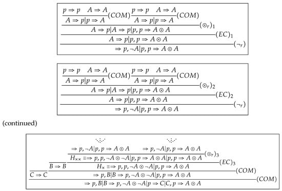
Figure 1.
A proof of .
By applying (D) to free combinations of all sequents in and in , we get that . is a theorem of and a cut-free proof of is shown in Figure 2. It supports the validity of the generalized density rule in Section 1, as an instance of .
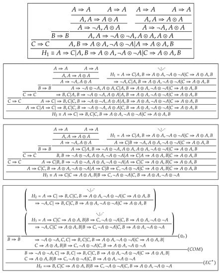
Figure 2.
A proof of .
Our task is to construct , starting from . The tree structure of is more complicated than that of . Compared with UL, MTL and IMTL, there is no one-to-one correspondence between nodes in and .
Following the method given by G. Metcalfe and F. Montagna, we need to define a generalized density rule for IUL. We denote such an expected unknown rule by for convenience. Then must be definable for all . Naturally,
However, we could not find a suitable way to define and for and in , see Figure 1. This is the biggest difficulty we encounter in the case of such that it is hard to prove density elimination for IUL. A possible way is to define as . Unfortunately, it is not a theorem of .
Notice that two upper hypersequents of are permissible inputs of . Why is an invalid input? One reason is that, two applications and cut off two sequents such that two disappear in all nodes lower than upper hypersequent of or , including . These make occurrences of to be incomplete in . We then perform the following operation in order to get complete occurrences of in .
Step 1 (preprocessing of ). Firstly, we replace H with for all , then replace with for all . Then we construct a proof without , which we denote by , as shown in Figure 3. We call such manipulations sequent-inserting operations, which eliminate applications of in .
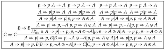
Figure 3.
A proof .
However, we also cannot define for in that . The reason is that the origins of in are indistinguishable if we regard all leaves in the form as the origins of which occur in the inner node. For example, we do not know which p comes from the left subtree of and which from the right subtree in two occurrences of in . We then perform the following operation in order to make all occurrences of in distinguishable.
We assign the unique identification number to each leaf in the form and transfer these identification numbers from leaves to the root, as shown in Figure 4. We denote the proof of resulting from this step by , where in which each sequent is a copy of some sequent in and in which each sequent is a copy of some external contraction sequent in -node of . We call such manipulations eigenvariable-labeling operations, which make us to trace eigenvariables in .
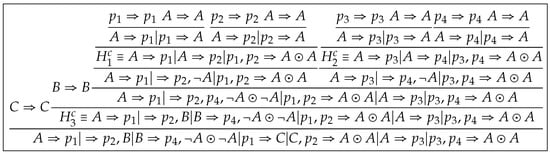
Figure 4.
A proof of .
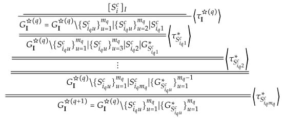
Then all occurrences of p in are distinguishable and we regard them as distinct eigenvariables (See Definition 18 (i)). Firstly, by selecting as the eigenvariable and applying to , we get
Secondly, by selecting and applying to , we get
Repeatedly, we get
We define such iterative applications of as -rule (See Definition 20). Lemma 10 shows that if . Then we obtain , i.e., .
A miracle happens here! The difficulty that we encountered in GIUL is overcome by converting into and using to replace .
Why do we assign the unique identification number to each ? We would return back to the same situation as that of if we assign the same indices to all or, replace and by in .
Note that . So we have built up a one-one correspondence between the proof of and that of . Observe that each sequent in is not a copy of any sequent in . In the following steps, we work on eliminating these sequents in .
Step 2 (extraction of elimination rules). We select as the focus sequent in in and keep unchanged from downward to (See Figure 4). So we extract a derivation from by pruning some sequents (or hypersequents) in , which we denote by , as shown in Figure 5.
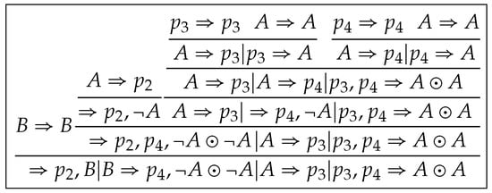
Figure 5.
A derivation from .
A derivation from is constructed by replacing with , with and with in , as shown in Figure 6. Notice that we assign new identification numbers to new occurrences of p in .
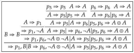
Figure 6.
A derivation from .
Next, we apply to in . Then we construct a proof , as shown in Figure 7, where .
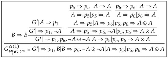
Figure 7.
A proof of .
However, contains more copies of sequents from and seems more complex than . We will present a unified method to tackle with it in the following steps. Other derivations are shown in Figure 8, Figure 9, Figure 10 and Figure 11.
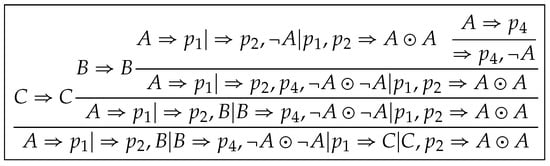
Figure 8.
A derivation from .
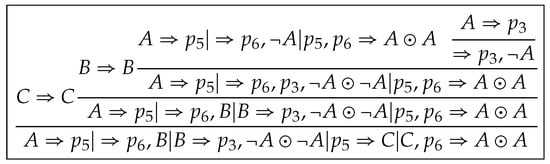
Figure 9.
A derivation from .
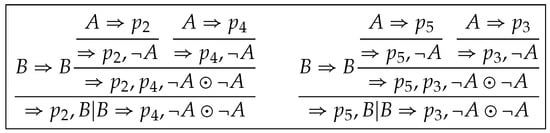
Figure 10.
and
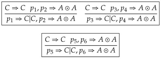
Figure 11.
, and .
Step 3 (separation of one branch). A proof is constructed by applying sequentially
to and in , as shown in Figure 12, where
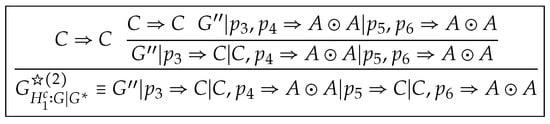
Figure 12.
A proof of .
Notice that
Then it is permissible to cut off the part
of , which corresponds to applying to . We regard such a manipulation as a constrained contraction rule applied to and denote it by . Define to be
Then we construct a proof of by , which guarantees the validity of
under the condition
A change happens here! There is only one sequent which is a copy of a sequent in in . It is simpler than . So we are moving forward. The above procedure is called the separation of as a branch of and reformulated as follows (See Section 7 for details).
The separation of as a branch of is constructed by a similar procedure as follows.
Note that and . So we have built up one-one correspondences between proofs of and those of .
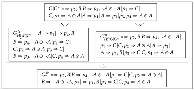
Step 3 (separation algorithm of multiple branches). We will prove in a direct way, i.e., only the major step of Theorem 2 is presented in the following. (See Appendix A.5.4 for a complete illustration.) Recall that
By reassigning identification numbers to occurrences of in ,
By applying to in and in , we get , where
Why reassign identification numbers to occurrences of in ? It makes different occurrences of to be assigned different identification numbers in two nodes and of the proof of .
By applying to , we get , where
A great change happens here! We have eliminated all sequents which are copies of some sequents in and converted into in which each sequent is some copy of a sequent in .
Then by Lemma 8, where =
So we have built up one-one correspondences between the proof of and that of , i.e., the proof of can be constructed by applying to the proof of . The major steps of constructing are shown in the following figure, where , , and .
In the above example, . But that is not always the case. In general, we can prove that if , which is shown in the proof of the main theorem in Page 42. This example shows that the proof of the main theorem essentially presents an algorithm to construct a proof of from .
4. Preprocessing of Proof Tree
Let be a cut-free proof of in the main theorem in by Lemma 1. Starting with , we will construct a proof which contains no application of and has some other properties in this section.
Lemma 2.
(i) If and
(ii) If and
Proof.
(i)
(ii) is proved by a procedure similar to that of (i) and omitted. □
We introduce two new rules by Lemma 2.
Definition 12.
and are called the generalized and rules, respectively.
Now, we begin to process as follows.
Step 1. A proof is constructed by replacing inductively all applications of
in with
The replacements in Step 1 are local and the root of is also labeled by .
Definition 13.
We sometimes may regard as a structural rule of and denote it by for convenience. The focus sequent for is undefined.
Lemma 3.
Let , , where and . A tree is constructed by replacing each in with for all . Then is a proof of .
Proof.
The proof is by induction on n. Since is a proof and is valid in , then is a proof. Suppose that is a proof. Since (or in , then (or is an application of the same rule (or ). Thus is a proof. □
Definition 14.
The manipulation described in Lemma 3 is called a sequent-inserting operation.
Clearly, the number of -applications in is less than . Next, we continue to process .
Step 2. Let be all applications of in and . By repeatedly applying sequent-inserting operations, we construct a proof of in without applications of and denote it by .
Remark 1.
(i) is constructed by converting into ; (ii) Each node of has the form , where and is a (possibly empty) subset of .
We need the following construction to eliminate applications of in .
Construction 1.
Let , and , where , . Hypersequents and trees for all are constructed inductively as follows.
(i) and consists of a single node ;
(ii) Let (or be in , and (accordingly for ) for some .
If
and is constructed by combining trees
otherwise and is constructed by combining
(iii) Let , and then and is constructed by combining
Lemma 4.
(i) for all ;
(ii) is a derivation of from without .
Proof.
The proof is by induction on k. For the base step, and consists of a single node . Then , is a derivation of from without .
For the induction step, suppose that and be constructed such that (i) and (ii) hold for some . There are two cases to be considered.
Case 1. Let , and . If then by . Thus Otherwise then by . Thus by . is a derivation of from without since is such one and is a valid instance of a rule of . The case of applications of the two-premise rule is proved by a similar procedure and omitted.
Case 2. Let , and . Then by . is a derivation of from without since is such one and is valid by Definition 13. □
Definition 15.
The manipulation described in Construction 1 is called a derivation-pruning operation.
Notation 3.
We denote by , by and say that is transformed into in .
Then Lemma 4 shows that , . Now, we continue to process as follows.
Step 3. Let then is a derivation of from thus a proof of is constructed by combining and with . By repeatedly applying the procedure above, we construct a proof of without in , where by Lemma 4(i).
Step 4. Let (or , then there exists such that for all (accordingly , thus a proof is constructed by replacing top-down p in each with ⊤.
Let (or , is a leaf of then there exists such that for all (accordingly or thus a proof is constructed by replacing top-down p in each with ⊥.
Repeatedly applying the procedure above, we construct a proof of in such that there does not exist occurrence of p in or at each leaf labeled by or , or p is not the weakening formula A in or when or is available. Define two operations and on sequents by and . Then is obtained by applying and to some designated sequents in .
Definition 16.
The manipulation described in Step 4 is called eigenvariable-replacing operation.
Step 5. A proof is constructed from by assigning inductively one unique identification number to each occurrence of p in as follows.
One unique identification number, which is a positive integer, is assigned to each leaf of the form in which corresponds to in . Other nodes of are processed as follows.
- Let . Suppose that all occurrences of p in are assigned identification numbers and have the form in , which we often write as Then has the form
- Let , where Suppose that and have the forms and in , respectively. Then has the form All applications of are processed by the procedure similar to that of .
- Let , whereSuppose that and have the forms and in , respectively. Then has the form All applications of are processed by the procedure similar to that of .
- Let , wherewhere , .
Suppose that and have the forms and in , respectively. Then has the form
where
for .
Definition 17.
The manipulation described in Step 5 is called eigenvariable-labeling operation.
Notation 4.
Let and be converted to G and in , respectively. Then is a proof of .
In the preprocessing of , each is converted into in Step 2, where by Lemma 3. is converted into in Step 3, where by Lemma 4(i). Some (or ) is revised as (or ) in Step 4. Each occurrence of p in is assigned the unique identification number in Step 5. The whole preprocessing above is depicted by Figure 13.
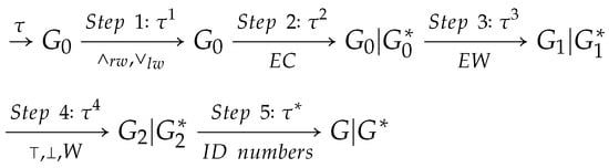
Figure 13.
Preprocessing of .
Notation 5.
Let be all -nodes of and be converted to in . Note that there are no identification numbers for occurrences of variable p in meanwhile they are assigned to p in . But we use the same notations for and for simplicity.
In the whole paper, let denote the unique node of such that and is the focus sequent of in , in which case we denote the focus one and others among . We sometimes denote also by or . We then write as .
We call , the i-th pseudo- node of and pseudo- sequent, respectively. We abbreviate pseudo- as Let , by we mean that for some .
It is possible that there does not exist such that is the focus sequent of in , in which case , then it has not any effect on our argument to treat all such as members of G. So we assume that all are always defined for all in , i.e., .
Proposition 2.
(i) for all ; (ii) .
Now, we replace locally each in with and denote the resulting proof also by , which has no essential difference with the original one, but could simplify subsequent arguments. We introduce the system as follows.
Definition 18.
is a restricted subsystem of such that
(i) p is designated as the unique eigenvariable by which we mean that it is not used to built up any formula containing logical connectives and only used as a sequent-formula.
(ii) Each occurrence of p on each side of every component of a hypersequent in is assigned one unique identification number i and written as in . Initial sequent of has the form in .
(iii) Each sequent S of in the form has the form
in , where p does not occur in Γ or Δ, for all , for all . Define and . Let G be a hypersequent of in the form then and for all . Define , . Here, l and r in and indicate the left side and right side of a sequent, respectively.
(iv) A hypersequent G of is called closed if . Two hypersequents and of are called disjoint if , , and . is a copy of if they are disjoint and there exist two bijections and such that can be obtained by applying to antecedents of sequents in and to succedents of sequents in , i.e., .
(v) A closed hypersequent can be contracted as in under the condition that and are closed and is a copy of . We call it the constraint external contraction rule and denote it by
Furthermore, if there do not exist two closed hypersequents such that is a copy of then we call it the fully constraint contraction rule and denote by .
(vi) and of are forbidden. , and of are replaced with , and in , respectively.
(vii) and are closed and disjoint for each two-premise rule
of and, is closed for each one-premise rule .
(viii) p does not occur in Γ or Δ for each initial sequent or and, p does not act as the weakening formula A in or when or is available.
Lemma 5.
Let τ be a cut-free proof of in and be the tree resulting from preprocessing of τ.
(i) If then ;
(ii) If then ;
(iii) If and then ;
(iv) If and (or ) then ;
(v) is a proof of in without ;
(vi) If and then , .
Proof.
Claims from (i) to (iv) follow immediately from Step 5 in preprocessing of and Definition 18. Claim (v) is from Notation 4 and Definition 18. Only (vi) is proved as follows.
Suppose that . Then , by Claim (iv). Thus or , a contradiction with hence .
is proved by a similar procedure and omitted. □
5. The Generalized Density Rule for
In this section, we define the generalized density rule for and prove that it is admissible in .
Definition 19.
Let G be a closed hypersequent of and . Define , i.e., is the minimal closed unit of G containing In general, for , define .
Clearly, if or p does not occur in S. The following construction gives a procedure to construct for any given .
Construction 2.
Let G and S be as above. A sequence of hypersequents is constructed recursively as follows. (i) ; (ii) Suppose that is constructed for . If then there exists (or thus there exists the unique such that (or by and Definition 18 then let otherwise the procedure terminates and .
Lemma 6.
(i) ;
(ii)Let then ;
(iii)Let , ,, , then , where is the symmetric difference of two multisets ;
(iv)Let then for all ;
(v)
Proof.
(i) Since for and then thus by . We prove for by induction on k in the following. Clearly, . Suppose that for some . Since (or and (or then by and thus . Then thus .
(ii) By (i), , where . Then for some thus (or hence there exists the unique such that (or if hence . Repeatedly, , i.e., then . by then .
(iii) It holds immediately from Construction 2 and (i).
(iv) The proof is by induction on k. For the base step, let then thus by . For the induction step, suppose that for some . Then by and . Then by .
(v) It holds by (iv) and . □
Definition 20.
Let and be in the form for .
(i) If and be then is defined as
(ii) Let and for all then is defined as .
(iii) We call the generalized density rule of , whose conclusion is defined by (ii) if its premise is G.
Clearly, is and if p does not occur in S.
Lemma 7.
Let and be closed and , where and Then
Proof.
Since then by , and Lemma 6 (iii). Thus , Hence
Therefore by
where . □
Lemma 8.
(Appendix A.5.1) If there exists a proof τ of G in then there exists a proof of in , i.e., is admissible in .
Proof.
We proceed by induction on the height of . For the base step, if G is then is otherwise is G then holds. For the induction step, the following cases are considered.
Case 1 Let
where
Then by , and Lemma 6(iii). Let then thus a proof of is constructed by combining the proof of and . Other rules of type are processed by a procedure similar to above.
Case 2 Let
where
Let
Then is
by . Then the proof of is constructed by combining and
with . All applications of are processed by a procedure similar to that of and omitted.
Case 3 Let
where
for Then , by Lemma 6 (iii). Let
for Then
for Then the proof of is constructed by combining and with . All applications of are processed by a procedure similar to that of and omitted.
Case 4 Let
where
where for
Case 4.1.. Then by Lemma 6(ii) and
by Lemma 6(iii). Then
Thus or . Hence we assume that, without loss of generality,
Then
Thus the proof of is constructed by
Case 4.2.. Then by Lemma 6(ii). Let
for Then
by , , and . Let
for Then
by Lemma 7, . Then the proof of is constructed by combing the proofs of and with
Case 5. Then and are closed and is a copy of thus hence a proof of is constructed by combining the proof of and . □
The following two lemmas are corollaries of Lemma 8.
Lemma 9.
If there exists a derivation of from in then there exists a derivation of from in .
Lemma 10.
Let τ be a cut-free proof of in and be the proof of in resulting from preprocessing of τ. Then .
6. Extraction of Elimination Rules
In this section, we will investigate Construction 1 further to extract more derivations from .
Any two sequents in a hypersequent seem independent of one another in the sense that they can only be contracted into one by when it is applicable. Note that one-premise logical rules just modify one sequent of a hypersequent and two-premise rules associate a sequent in a hypersequent with one in a different hypersequent.
(or any proof without in ) has an essential property, which we call the distinguishability of , i.e., any variables, formulas, sequents or hypersequents which occur at the node H of occur inevitably at in some forms.
Let . If is equal to as two sequents then the case that is equal to as two derivations could possibly happen. This means that both and are the focus sequent of one node in when and , which contradicts that each node has the unique focus sequent in any derivation. Thus we need to differentiate from for all .
Define such that , and is the principal sequent of . If has the unique principal sequent, , otherwise (or to indicate that is one designated principal sequent (or accordingly for another) of such an application as or . Then we may regard as . Thus is always different from by or, and . We formulate it by the following construction.
Construction 3.
(Appendix A.5.2) A labeled tree , which has the same tree structure as , is constructed as follows.
(i) If S is a leaf , define , and the node of is labeled by ;
(ii) If and be labeled by in . Then define , and the node of is labeled by ;
(iii) If , and be labeled by and in , respectively. If then define , , and the node of is labeled by . If then define , and is labeled by .
In the whole paper, we treat as without mention of . Note that in preprocessing of , some logical applications could also be converted to in Step 3 and we need fix the focus sequent at each node H and subsequently assign valid identification numbers to each by eigenvariable-labeling operation.
Proposition 3.
(i) implies ; (ii) and imply ; (iii) Let and then or .
Proof.
(iii) Let then for some by Notation 5. Thus also by Notation 5. Hence and by Construction 3. Therefore or . □
Lemma 11.
Let and , where , , for .
(i) If then for all ;
(ii) If then for all .
Proof.
The proof is by induction on i for . Only (i) is proved as follows and (ii) by a similar procedure and omitted.
For the base step, holds by , , and .
For the induction step, suppose that for some . Only is the case of a one-premise rule given in the following and other cases are omitted.
Let , and .
Let . Then , by and
Thus
Let and . Then ,
Thus
Let . Then ,
Thus
The case of is proved by a similar procedure and omitted. □
Lemma 12.
(i) Let then
(ii) , then .
Proof.
(i) and (ii) are immediately from Lemma 11. □
Notation 6.
We write , as , , respectively, for the sake of simplicity.
Lemma 13.
(i) ;
(ii) is a derivation of from , which we denote by ;
(iii) and consists of a single node for all ;
(iv) ;
(v) implies . Note that is undefined for any or .
(vi) implies .
Proof.
Claims from (i) to (v) follow immediately from Construction 1 and Lemma 4.
(vi) Since then has the form for some by Notation 5. Then by (iii). Suppose that . Then is transferred from downward to and in side-hypersequent of by Notation 5 and . Thus at since is the unique focus sequent of . Hence by Lemma 11 and (iii), a contradiction therefore . □
Lemma 14.
Let . (i) If then or ; (ii) If then or .
Proof.
(i) We impose a restriction on such that each sequent in is different from or otherwise we treat it as an -application. Since then has the form for some by Notation 5. Thus . Suppose that . Then is transferred from downward to H. Thus by and Lemma 11. Hence or , a contradiction with the restriction above. Therefore or .
(ii) Let . If then by Proposition 2(i) and thus by Lemma 11 and, hence by , . If then by . Thus or . □
Definition 21.
(i) By we mean that for some ; (ii) By we mean that and ; (iii) means that for all .
Then Lemma 13(vi) shows that implies .
Lemma 15.
Let , , such that , . Then .
Proof.
Suppose that . Then by , by Construction 1. Thus . Hence by Proposition 3(ii). Therefore for all by Lemma 11, i.e., , a contradiction and hence . □
Lemma 13(ii) shows that is a derivation of from one premise . We generalize it by introducing derivations from multiple premises in the following. In the remainder of this section, let , for all . Then and by Lemma 13(vi) thus for all .
Notation 7.
denotes the intersection node of . We sometimes write the intersection node of and as . If , , i.e., the intersection node of a single node is itself.
Let such that . Then I is divided into two subsets and , which occur in the left subtree and right subtree of , respectively.
Let , , such that . A derivation of from is constructed by induction on . The base case of has been done by Construction 1. For the induction case, suppose that derivations of from and of from are constructed. Then of from is constructed as follows.
Construction 4.
(ii)
and
(iii) Other nodes of are built up by Construction 1(ii).
The following lemma is a generalization of Lemma 13.
Lemma 16.
Let , where and . Then, for all ,
(i)
(ii)
(iii)
(iv) if and only if for some . Note that is undefined if or for all .
Proof.
(i) is proved by induction on . For the base step, let then the claim holds clearly. For the induction step, let then and . Then for all by Lemma 15 and for all . by the induction hypothesis then thus by .
holds by a procedure similar to above then
by and . Other claims hold immediately from Construction 4. □
Lemma 17.
(i) Let denote then ;
(ii)
(iii) ;
(iv) implies for all .
Proof.
(i), (ii) and (iii) follow immediately from Lemma 16. (iv) holds by (i) and Lemma 13 (vi). □
Lemma 17 (iv) shows that there exists no copy of in for any . Then we may regard them to be eliminated in . We then call an elimination derivation.
Let be another set of sequents to I such that is a copy of . Then and are disjoint and there exist two bijections and such that . By applying to , we construct a derivation from and denote it by and its root by .
Let be a set of hypersequents to I, where be closed for all . By applying to in , we construct a derivation from
and denote it by and its root by . Then .
Definition 22.
We will use all as rules of and call them elimination rules. Further, we call focus sequents and, all sequents in principal sequents and, side-hypersequents of .
Remark 2.
We regard Construction 1 as a procedure , whose inputs are and output . With such a viewpoint, we write as . Then can be constructed by iteratively applying to , i.e., .
We replace locally each in with and denote the resulting derivation also by . Then each non-root node in has the focus sequent.
Let . Then there exists a unique node in , which we denote by such that H comes from by Constructions 1 and 4. Then the focus sequent of in is the focus of H in if H is a non-root node and, or as two hypersequents. Since the relative positions of any two nodes in are kept unchanged in constructing , if and only if for any . Especially, for .
Let . Then and . Define . Then and for all .
Since , then each -sequent in has the form for some , by Proposition 2(ii). Then we introduce the following definition.
Definition 23.
(i) By we means that there exists such that , . So is .
(ii) Let . By we means that there exist such that , and . We usually write as ⩽.
7. Separation of One Branch
In the remainder of this paper, we assume that p occur at most one time for each sequent in as the one in the main theorem, be a cut-free proof of in and the proof of in resulting from preprocessing of . Then for all , which plays a key role in discussing the separation of branches.
Definition 24.
By we mean that there exists some copy of in . if for all . if and . Let be m copies of then we denote by or .
Definition 25.
Let , for all . is called a branch of to I if it is a closed hypersequent such that
implies or for all
Then (i) for all , ; (ii) and imply .
In this section, let , , we will give an algorithm to eliminate all satisfying .
Construction 5.
(Appendix A.3) A sequence of hypersequents and their derivations from for all are constructed inductively as follows.
For the base case, define to be and, be . For the induction case, suppose that and are constructed for some . If there exists no such that , then the procedure terminates and define to be q; otherwise define such that , and for all . Let be all copies of in then define and its derivation is constructed by sequentially applying to in , respectively. Notice that we assign new identification numbers to new occurrences of p in for all , .
Lemma 18.
(i) and for all ;
(ii) is closed for all ;
(iii) for all , especially, ;
(iv) implies and, for some or , , where , is closed and , .
Proof.
(i) Since by and, for all then . If then by , thus by all copies of in being collected in . If then by Lemma 13(vi) thus by , . Then by . Note that is undefined in Construction 5.
(ii) by . Suppose that then by , and for all .
(iii) is . Given then is constructed by linking up the conclusion of previous derivation to the premise of its successor in the sequence of derivations
as shown in Figure 14.
Figure 14.
A derivation of from .
(iv) Let . Then by the definition of . If , then by and the definition of . Otherwise, by Construction 5, there exists some in such that Then by Lemma 13(vi). Thus by . Hence . □
Lemma 18 shows that Construction 5 presents a derivation of from such that there does not exist satisfying , i.e., all satisfying are eliminated by Construction 5. We generalize this procedure as follows.
Construction 6.
Let , and . Then and its derivation for are constructed by procedures similar to that of Construction 5 such that for all , where , , which are defined by Construction 1.
We sometimes write , as J for simplicity. Then the following lemma holds clearly.
Lemma 19.
(i) , for all .
(ii) If and then .
(iii) If or, is a copy of and then .
(iv) Let . Then by suitable assignments of identification numbers to new occurrences of p in constructing , and .
(v) .
Proof.
Part (i) is proved by a procedure similar to that of Lemma 18(iii) and (iv), and omitted.
(ii) Since is the focus sequent of then it is revised by some rule at the node lower than . Thus is some copy of by . Hence has the form for some . Therefore it is transferred downward to , i.e., . Then . Since there exists no then . Thus .
(iii) is proved by a procedure similar to that of (ii) and omitted.
(iv) Since , then by Proposition 3. Thus . Suppose that for some . Then all copies of in are divided two subsets and . Thus we can construct and simultaneously and assign the same identification numbers to new occurrences of p in and as the corresponding one in . Hence . Then .
Note that the requirement is imposed only on one derivation that distinct occurrence of p has a distinct identification number. We permit or in the proof above, which has no essential effect on the proof of the claim.
(v) is immediately from (iv). □
Lemma 19 (v) shows that could be constructed by applying sequentially to each satisfying . Thus the requirement in Construction 5 is not necessary, but which make the termination of the procedure obvious.
Construction 7.
Apply to and denote the resulting hypersequent by and its derivation by . It is possible that is not applicable to in which case we apply to it for the regularity of the derivation.
Lemma 20.
(i) , is closed and for all ;
(ii) is constructed by applying elimination rules, say, , and the fully constraint contraction rules, say, , where , is closed for , .
Proof.
The proof follows immediately from Lemma 18. □
Definition 26.
Let , and .
(i) For any sequent-formula A of , define to be the sequent S of such that A is a sequent-formula of S or subformula of a sequent-formula of S.
(ii) Let be in the form , define to be the hypersequent which consists of all distinct sequents among ; (iii) Let be in the form , define to be .
(iv) We call to be separable if and, call it to be separated into .
Note that is a derivation without in . Then we can extract elimination derivations from it by Construction 1.
Notation 8.
Let . denotes the derivation from , which extracts from by Construction 1, and denote its root by .
The following two lemmas show that Constructions 5 and 6 force some sequents in or to be separable.
Lemma 21.
Let . Then
(i) is separable in .
(ii) If , then is separable in and there is a unique copy of in .
Proof.
(i) We write and respectively as and ⩽ for simplicity. Since , we divide it into two hypersequents and such that .
Let then by Construction 6. We prove that in as follows. If then in by Lemma 14(i), and . Thus we assume that in the following.
Then, by Lemma 18(iv), there exists some in such that , . Then by Lemma 13(vi). by , . Thus . Let , where , , . Then , , by . Thus by , and .
Thus in . Therefore . Then , i.e., is separable in .
(ii) Clearly, is a copy of and, has no difference with except some applications of and identification numbers of some . Then is separated into in by the same reason as that of (i). Then are separated into and in , respectively. Then is closed since is closed. Thus all copies of in are contracted into one by in . □
Lemma 22.
(i) All copies of in are separable in .
(ii) Let , , or for all . Then is separable in .
Proof.
Parts (i) and (ii) are proved by a procedure similar to that of Lemma 21 and are omitted. □
Definition 27.
The skeleton of , which we denote by , is constructed by replacing all with , i.e, is the parent node of in .
Lemma 23.
The parameter is a linear structure with the lowest node and the highest .
Proof.
It holds by all and in being one-premise rules. □
Definition 28.
We call Construction 5 together with 7 the separation algorithm of one branch and, Construction 6 the separation algorithm along H.
8. Separation Algorithm of Multiple Branches
In this section, let such that for all . We will generalize the separation algorithm of one branch to that of multiple branches. Roughly speaking, we give an algorithm to eliminate all satisfying for some .
Definition 29.
.
Theorem 2.
Let . Then there exist one closed hypersequent and its derivation from , …, in such that
(i) is constructed by applying elimination rules, say,
and the fully constraint contraction rules, say , where , for all , , , and is closed for all . Then for all and .
(ii) For all ,
where, is the skeleton of which is defined as Definition 27. Then
for some in .
(iii) Let , , then and it is constructed by applying the separation algorithm along to H and, is an upper hypersequent of either if it is applicable, or otherwise.
(iv) implies for all and, for some or for some satisfying .
Note that in Claim (i), bold in or indicates the w-tuple in . Claim (iv) shows the final aim of Theorem 2, i.e., there exists no such that for some . It is almost impossible to construct in a non-recursive way. Thus we use Claims (i)–(iii) in Theorem 2 to characterize the structure of in order to construct it recursively.
Proof.
is constructed by induction on . For the base case, let . Then is constructed by Construction 5 and 7. Here, Claim (i) holds by Lemma 20(ii), Lemma 18(i) and Lemma 13(vi), Claim (ii) by Lemma 18(i), (iii) is clear and (iv) by Lemma 18(iv).
For the induction case, let . Let , where . Then is divided into two subsets which occur in the left subtree and right subtree of , respectively. Then . Let Suppose that derivations of and of are constructed such that Claims from (i) to (iv) hold. There are three cases to be considered in the following.
Case 1. for all . Then and .
- For Claim (i), let and . By the induction hypothesis, for all . Since then . Thus by Lemmas 11 and 12. Then . Thus by Proposition 2(i). Hence, for all , by . Then for all . Claims (ii) and (iii) follow directly from the induction hypothesis.
- For Claim (iv), let . It follows from the induction hypothesis that for all and, for some or for some . Then by .
If for some then for all by the definition of branches to I. Thus we assume that for some in the following. If then for all thus for all . Thus let in the following. By the proof of Claim (i) above, . Then by and . Thus . Hence for all .
Case 2. for all . Then and . This case is proved by a procedure similar to that of Case 1 and omitted.
Case 3. for some and for some .
Given
such that and for all , where, , is closed for all , Then by and for all . Thus for all and by and Construction 4.
For each above, we construct a derivation in which you may regard as a subroutine, and as its input in the following stage 1. Then a derivation is constructed by calling in Stage 2, in which you may regard as a routine and as its subroutine.
Before proceeding to deal with Case 3, we present the following property of which are derived from Claims (i) ∼ (iv) and applicable to or under the induction hypothesis.
Notation 9.
Let
be two close hypersequents, for some and for some .
Generally, is a copy of , i.e., eigenvariables in have different identification numbers with those in , so are .
Lemma 24.
implies .
Proof.
Let . Then by Lemma 19(i). Thus or . If then by and Proposition 1 (ii). If then by Proposition 2(i). Thus by Lemma 11, Lemma 14(i). Hence by , . □
Lemma 25.
(1) is an m-ary tree and, is a binary tree;
(2) Let then for some ;
(3) Let then ;
(4) Let in then for all .
(5) Let , for some . Then .
Proof.
(1) is immediately from Claim (i). (2) holds by and for some by . (3) holds by Proposition 1(iii), (2) and .
For (4), let . Then for each , and for some by (2). Thus and by Proposition 1(ii). Hence by , and by . Thus and by (3), . Hence for all . (5) is from (4). □
Lemma 26.
Let for all such that and . Then and for all .
Proof.
The proof is by induction on n. Let then by Lemma 25(5) and . For the induction step, let for some then by Lemma 25(5). Since then for some by Claim (ii). Then by . Thus by Lemma 25(5). □
Definition 30.
Let . The module of at , which we denote by , is defined as follows: (1) ; (2) if ; (3) if , .
Each node of is determined bottom-up, starting with , whose root is and leaves may be branches, leaves of or lower hypersequents of -applications. While each node of is determined top-down, starting with , whose root is a subset of and leaves contain and some leaves of .
Lemma 27.
(1) is a derivation without in .
(2) Let and . Then for all and .
Proof.
Part (1) is clear and (2) immediately follows from Lemma 26. □
Now, we continue to deal with Case 3 in the following.
Stage 1 Construction of Subroutine Roughly speaking, is constructed by replacing some nodes with in post-order. However, the ordinal postorder-traversal algorithm cannot be used to construct because the tree structure of is generally different from that of at some nodes satisfying . Thus we construct a sequence of trees for all inductively as follows.
For the base case, we mark all -applications in as unprocessed and define such marked derivation to be . For the induction case, let be constructed. If all applications of in are marked as processed, we firstly delete the root of the tree resulting from the procedure and then, apply to the root of the resulting derivation if it is applicable otherwise add an -application to it and finally, terminate the procedure. Otherwise we select one of the outermost unprocessed -applications in , say, , and perform the following steps to construct in which be revised as such that
(a) is constructed by locally revising and leaving other nodes of unchanged, particularly including ;
(b) is a derivation in ;
(c) if for all otherwise
for some .
Remark 3.
By two superscripts ∘ and · in or , we indicate the unprocessed state and processed state, respectively. This procedure determines an ordering for all -applications in and the subscript indicates that it is the -th application of in a post-order transversal of . and ( and ) are the premise and conclusion of (), respectively.
Step 1 (Delete). Take the module out of . Since is the unique unprocessed -applications in by its choice criteria, is the same as by Claim (a). Thus it is a derivation. If for all , delete all internal nodes of . Otherwise there exists
such that for all and by Lemma 27(2) and , then delete all , . We denote the structure resulting from the deletion operation above by . Since then is a tree by Lemma 26. Thus it is also a derivation.
Step 2 (Update). For each which satisfies and for some , we replace H with for each , .
Since and is the outermost unprocessed
-application in then and has been processed. Thus Claims (b) and (c) hold for by the induction hypothesis. Then is a valid -application since , and are valid, where , .
Lemma 28.
Let . Then .
Proof.
Since then for some . If then . Otherwise all applications between and H are one-premise rules by Lemma 26. Then by Claim (ii). Thus by , for some by Claim (i). □
Since by Lemma 28 and for each by Lemma 24, then as side-hypersequent of H. Thus this step updates the revision of downward to .
Let be the number of satisfying the above conditions, , and for all be updated as , , , respectively. Then is a derivation and .
Step 3 (Replace). All are processed in post-order. If for all and it proceeds by the following procedure otherwise it remains unchanged. Let be in the form
Then for all by Lemma 28, .
Firstly, replace with . We may rewrite the roots of and as
respectively.
Let . By Lemma 28, . By Lemma 14, or for all . Thus . Secondly, we replace H with for all . Let be the number of satisfying the replacement conditions above, , and for all be updated as , , , respectively. Then is a derivation of and
Step 4 (Separation along ). Apply the separation algorithm along to and denote the resulting derivation by whose root is labeled by . Then all in are transformed into in . Since
, and are separable in by a procedure similar to that of Lemma 21. Let and be separated into and , respectively. By Claim (iii),
where .
Step 5 (Put back). Replace in with and mark as processed, i.e., revise as . Among leaves of , all are updated as and others keep unchanged in . Then this replacement is feasible, especially, be replaced with . Define the tree resulting from Step 5 to be . Then Claims (a), (b) and (c) hold for by the above construction.
Finally, we construct a derivation of from , in , which we denote by .
Remark 4.
All elimination rules used in constructing are extracted from . Since is a derivation in without , we may extract elimination rules from which we may use to construct by a procedure similar to that of constructing with minor revision at every node H that . Note that updates and replacements in Steps 2 and 3 are essentially inductive operations but we neglect it for simplicity.
We may also think of constructing as grafting in by adding to some . Since the rootstock of the grafting process is invariant in Stage 2, we encapsulate as an rule in whose premises are and conclusion is , i.e.,
where, is closed.
Stage 2. Construction of routine . A sequence of trees for all is constructed inductively as follows. , , are defined as those of Stage 1. Then we perform the following steps to construct in which be revised as such that Claims (a) and (b) are same as those of Stage 1 and (c) if for all otherwise for some .
Step 1 (Delete). and are defined as before.
satisfies for all and .
Step 2 (Update). For all which satisfy and for some , we replace H with for all , . Then Claims (a) and (b) are proved by a procedure as before. Let be the number of satisfying the above conditions. , and for all be updated as , , , respectively. Then is a derivation and .
Step 3 (Replace). All are processed in post-order. If for all and it proceeds by the following procedure otherwise it remains unchanged. Let be in the form
Then there exists the unique such that .
Firstly, we replace with . We may rewrite the roots of , as respectively.
Let . Then by Lemma 28. Thus Define .
Then we replace H with
for all .
Let be the number of satisfying the replacement conditions as above, , and for all be updated as , , , respectively. Then is a derivation and , where
Step 4 (Separation along ). Apply the separation algorithm along to and denote the resulting derivation by whose root is labeled by .
By Claim (iii), .
Then
Then
where .
Step 5 (Put back). Replace in with and revise as . Define the resulting tree from Step 5 to be then Claims (a), (b) and (c) hold for by the above construction.
Finally, we construct a derivation of from , …, in . Since the major operation of Stage 2 is to replace with for all satisfying , then we denote the resulting derivation from Stage 2 by .
In the following, we prove that the claims from (i) to (iv) hold if and .
- For Claims (i) and (ii): Let and . Then for all by Lemma 17(iv).If for some , then for all by . Thus Claim (i) holds and Claim (ii) holds by Lemma 25(5) and Lemma 19(i). Note that Lemma 25(5) is independent of Claims from (ii) to (iv).Otherwise is built up from , or by keeping their focus and principal sequents unchanged and making their side-hypersequents possibly to be modified, but which has no effect on discussing Claim (ii) and then Claim (ii) holds for by the induction hypothesis on Claim (ii) of or .If is from then and by the choice of and at Stage 1. By the induction hypothesis, for all and for all . Then for all , by , .If is from then by Step 3 at Stage 1. Then . Thus . Hence . Therefore for all by . Thus for all by and the induction hypothesis from . The case of built up from is proved by a procedure similar to above and omitted.
- Claim (iii) holds by Step 4 at Stages 1 and 2. Note that in the whole of Stage 1, we treat as a side-hypersequent. But it is possible that there exists such that . Since we have not applied the separation algorithm to in Step 4 at Stage 1, then it could make Claim (iii) invalid. But it is not difficult to find that we just move the separation of such to Step 4 at Stage 2. Of course, we can move it to Step 4 at Stage 1, but which make the discussion complicated.
- For Claim (iv), we prove (1) for all and , (2) for all and . Only (1) is proved as follows and (2) by a similar procedure and omitted.
Let . Then and by the definition of . By a procedure similar to that of Claim (iv) in Case 1, we get and assume that for some and let in the following.
Suppose that . Then and by . Hence by . Therefore , a contradiction thus . Then by and . Thus . Hence for all . This completes the proof of Theorem 2. □
Definition 31.
The manipulation described in Theorem 2 is called a derivation-grafting operation.
9. The Proof of the Main Theorem
Recall that in the main theorem
Lemma 29.
(i) If and then ;
If and then ;
(ii) If and then ;
If and then ;
(iii) If and then ;
If and then .
Proof.
(i) Since then holds. If , we replace all p in with ⊥. Then holds by applying to and
(ii) Since then holds by applying to .
(iii) Since then holds by applying to in and . Thus holds by applying to .
and are proved by a procedure respectively similar to those of (i), (ii) and (iii) and omitted. □
Let , denote a closed hypersequent such that and for all and .
Lemma 30.
There exists such that for all .
Proof.
The proof is by induction on m. For the base step, let , then and and by Lemma 5 (v).
For the induction step, suppose that and there exists such that for all . Then there exist for all such that and for all and .
If for all then and the claim holds clearly. Otherwise there exists such that or then we rewrite as , where we define such that and, implies or for all . If we cannot define to be for each , let . Then is constructed by applying the separation algorithm of multiple branches (or one branch if ) to . Then by , Theorem 2 (or Lemma 20(i) for one branch). Let then clearly. □
The proof of Theorem 1:
Let in Lemma 30. Then there exists such that , and for all and . Then by Lemma 8.
Suppose that . Then for all . Thus by , a contradiction with and hence there does not exist . Therefore by .
By removing the identification number of each occurrence of p in G, we obtain the sub-hypersequent of , which is the root of resulting from Step 4 in Section 4. Then by and . Since is constructed by adding or removing some or from , or replacing with , or with , then by Lemma 29. This completes the proof of the main theorem. □
Theorem 3.
Density elimination holds for all in
Proof.
It follows immediately from the main theorem. □
10. Final Remarks and Open Problems
Recently, we have generalized our method described in this paper to the non-commutative substructural logic in [20]. This result shows that is the logic of pseudo-uninorms and their residua and answered the question posed by Metcalfe, Olivetti, Gabbay and Tsinakis in [21,22].
It has often been the case in the past that metamathematical proofs of the standard completeness have the corresponding algebraic ones, and vise verse. In particular, Baldi and Terui [23] had given an algebraic proof of the standard completeness of UL. A natural problem is whether there is an algebraic proof corresponding to our proof-theoretic one. It seems difficult to obtain it by using the insights gained from the approach described in this paper because ideas and syntactic manipulations introduced here are complicated and specialized. In addition, Baldi and Terui [23] also mentioned some open problems. Whether our method could be applied to their problems is another research direction.
On 21 March 2014, I found the way to deal with the example in Section 3. Then I finished the one branch algorithm in Section 7 on the late April 2014. I devised the multi-branch algorithm in Section 8 on early November 2014. Since I submitted my paper to Transactions of the American Mathematical Society on 20 January 2015, it has been reviewed successively by Annals of Pure and Applied Logic, Fuzzy Sets and Systems and, the Journal of Logic and Computation. As a mathematician, the greatest anxiety is that his work has never been taken seriously by his academic circle during his career, but after his death, someone would say, sir, your proof is wrong.
Funding
This research was funded by the National Foundation of Natural Sciences of China (Grant No: 61379018 &61662044& 11571013&11671358).
Acknowledgments
I am grateful to Lluis Godo, Arnon Avron, Jean-Yves Girard, George Metcalfe and Agata Ciabattoni for valuable discussions. I would like to thank anonymous reviewers for carefully reading the old version of this article and many instructive suggestions.
Conflicts of Interest
The authors declare no conflict of interest.
Notations
| The symbol denotes a complex hypersequent temporarily for convenience. | |
| Define X as Y for two hypersequents (sets or derivations) X and Y. | |
| The upper hypersequent of strong density rule in Theorem 1, page 2 | |
| A cut-free proof of in , in Theorem 1, page 3 | |
| The position of , Def. 10, Construction 3, pages 5, 24 | |
| and | Construction 1, page 15 |
| and | Notation 3, page 16 |
| The proof of in resulting from preprocessing of , Notation 4, page 17 | |
| The root of corresponding to the root of , Notation 4, page 17 | |
| The i-th -node in , the superscript means contraction, Notation 5, page 18 | |
| The focus sequent of , Notation 5, page 18 | |
| or | or one copy of , Notation 5, page 18 |
| The set of all -nodes in , Notation 5, page 18 | |
| A restricted subsystem of , Definition 18, page 18 | |
| The minimal closed unit of S and in G, respectively, Definition 19, page 19 | |
| The generalized density rule of , Definition 20, page 20 | |
| and | Notation 6, Page 25 |
| Definition 21, page 25 | |
| A subset of , Notation 7, page 26 | |
| , | The intersection nodes of I and, that of and , Notation 7, page 26 |
| A subset of -sequents to I, Definition 22, page 27 | |
| A set of closed hypersequents to I, Definition 22, page 27 | |
| and | The elimination derivation, Construction 4, Lemma 17, pages 26, 27 |
| The elimination rule, Definition 22, page 27 | |
| A branch of to I, Definition 25, page 28 | |
| Construction 5, page 28 | |
| Construction 6, page 30 | |
| Construction 7, Theorem 2, pages 31, 32 | |
| The skeleton of , Definition 27, page 32 | |
| Theorem 2 (ii), page 33 | |
| The module of at , Definition 30, page 35 |
Appendix A.
Appendix A.1. Why Do We Adopt Avron-Style Hypersequent Calculi?
A hypersequent calculus is called Pottinger-style if its two-premise rules are in the form of and, Avron-style if in the form of . In the viewpoint of Avron-style systems, each application of two-premise rules contains implicitly applications of in Pottinger-style systems, as shown in the following.
The choice of the underlying system of hypersequent calculus is vital to our purpose and it gives the background or arena. In Pottinger-style system, in Section 3 is proved without application of as follows. But it seems helpless to prove that is a theorem of IUL.
The peculiarity of our method is not only to focus on controlling the role of the external contraction rule in the hypersequent calculus but also introduce other syntactic manipulations. For example, we label occurrences of the eigenvariable p introduced by an application of the density rule in order to be able to trace these occurrences from the leaves (axioms) of the derivation to the root (the derived hypersequent).
Appendix A.2. Why Do We Need the Constrained External Contraction Rule?
We use the example in Section 3 to answer this question. Firstly, we illustrate Notation 5 as follows. In Figure 4, let Then for . are -nodes and, and are -sequents.
Let . We denote the derivation of from by . Since we focus on sequents in in the separation algorithm, we abbreviate to and further to . Then the separation algorithm is abbreviated as
where and are abbreviations of and , respectively. We also write and respectively as 2 and 3 for simplicity. Then the whole separation derivation is given as follows.
where ∅ is an abbreviation of in page 14 and means that all sequents in it are copies of sequents in . Note that the simplified notations become intractable when we decide whether is applicable to resulting hypersequents. If no application of is used in it, all resulting hypersequents fall into the set and ∅ is never obtained.
Appendix A.3. Why Do We Need the Separation of Branches?
In Figure 11, and in the premise of could be viewed as being tangled in one sequent but in the conclusion of they are separated into two sequents and , which are copies of sequents in . In Figure 5, in falls into in the root of and is a copy of a sequent in . The same is true for in in Figure 8. But it’s not the case.
Lemma 13(vi) shows that in the elimination rule , implies or . If there exists no such that , then implies and, thus each occurrence of in is fell into a unique sequent which is a copy of a sequent in . Otherwise there exists such that , then we apply to in and the whole operations can be written as
Repeatedly we can get such that implies . Then each occurrence of in is fell into a unique sequent in which is a copy of a sequent in . In such case, we call occurrences of in are separated in and call such a procedure the separation algorithm. It is the starting point of the separation algorithm. We introduce branches in order to tackle the case of multiple-premise separation derivations for which it is necessary to apply to the resulting hypersequents.
Appendix A.4. Some Questions about Theorem 2
In Theorem 2, is constructed by induction on the number of branches. As usual, we take the algorithm of branches as the induction hypothesis. Why do we take and as the induction hypothesises?
Roughly speaking, it degenerates the case of branches into the case of two branches in the following sense. The subtree of is as a whole contained in or not in it. Similarly, of is as a whole contained in or not in it. It is such a division of I into and that makes the whole algorithm possible.
Claim (i) of Theorem 2 asserts that for all and . It guarantees that is not far from the final aim of Theorem 2 but roughly close to it if we define some complexity to calculate it. If , the complexity of is more than or equal to that of under such a definition of complexity and thus such an application of is redundant at least. Claim (iii) of Theorem 2 guarantees the validity of the step 4 of Stages 1 and 2.
The tree structure of the skeleton of can be obtained by deleting some node satisfying . The same is true for if is treated as a rule or a subroutine whose premises are same as ones of . However, it is incredibly difficult to imagine or describe the structure of if you want to expand it as a normal derivation, a binary tree.
All syntactic manipulations in constructing are performed on the skeletons of or . The structure of the proof of Theorem 2 is depicted in Figure A1.
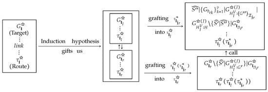
Figure A1.
The structure of the proof of Theorem 2.
Appendix A.5. Illustrations of Notations and Algorithms
We use the example in Section 3 to illustrate some notations and algorithms in this paper.
Appendix A.5.1. Illustration of Two Cases of (COM) in the Proof of Lemma 8
Let be , where ; ; ; and . Then ; ; ; . Thus the proof of is constructed by .
Let be
;
; ; ; and . Then ; ; ; .
Thus the proof of is constructed by
Appendix A.5.2. Illustration of Construction 3
Let be
By Construction 3, is then given as follows.
As an example, we calculate . Since , then , by Definition 10. Thus
Note that we cannot distinguish the one from the other for two in . If we divide into , where and , then in the conventional meaning of hypersequents. Thus only in the sense that we treat as , the assertion that for any in Proposition 3 holds.
Appendix A.5.3. Illustration of Notation 7 and Construction 4
Let
where (See Figure 4).
(See Figure 5).
(See Figure 8).
(See Figure 10).
Appendix A.5.4. Illustration of Theorem 2
Note that sequents in are principal sequents of elimination rules in the following. Let be the same as in Appendix A.5.3 and,
where
where
Since there is only one elimination rule in , the case we need to process is , i.e.,
Then , ;
where , , , , .
Since there is only one elimination rule in , the case we need to process is , i.e.,
Then , ;
is replaced with in Step 3 of Stage 1, i.e.,
where
Replacing in with , then deleting and after that applying to and keeping unchanged, we get
where ; ;
Stage 2
Replacing in with , then deleting and after that applying to , we get .
References
- Rose, A.; Rosser, J.B. Fragments of many-valued statement calculi. Trans. Am. Math. Soc. 1958, 87, 1–53. [Google Scholar]
- Chang, C.C. Algebraic analysis of many-valued logics. Trans. Am. Math. Soc. 1958, 88, 467–490. [Google Scholar]
- Chang, C.C. A new proof of the completeness of the Lukasiewicz’s axioms. Trans. Am. Math. Soc. 1959, 93, 74–80. [Google Scholar] [CrossRef]
- Hájek, P. Metamathematics of Fuzzy Logic; Kluwer: Dordrecht, The Netherlands, 1998. [Google Scholar]
- Hájek, P. Basic fuzzy logic and BL-algebras. Soft Comput. 1998, 2, 124–128. [Google Scholar] [CrossRef]
- Cignoli, R.; Esteva, F.; Godo, L.; Torrens, A. Basic fuzzy logic is the logic of continuous t-norms and their residua. Soft Comput. 2000, 4, 106–112. [Google Scholar] [CrossRef]
- Esteva, F.; Godo, L. Monoidal t-norm based logic: towards a logic for left-continuous t-norms. Fuzzy Sets Syst. 2001, 124, 271–288. [Google Scholar] [CrossRef]
- Jenei, S.; Montagna, F. A proof of standard completeness for Esteva and Godo’s logic MTL. Stud. Log. 2002, 70, 183–192. [Google Scholar] [CrossRef]
- Metcalfe, G.; Montagna, F. Substructural fuzzy logics. J. Symb. Log. 2007, 7, 834–864. [Google Scholar] [CrossRef]
- Cintula, P.; Noguera, C. Implicational (semilinear) logics I: A new hierarchy. Arch. Math. Log. 2010, 49, 417–446. [Google Scholar] [CrossRef]
- Takeuti, G.; Titani, T. Intuitionistic fuzzy logic and intuitionistic fuzzy set theory. J. Symb. Log. 1984, 49, 851–866. [Google Scholar] [CrossRef]
- Avron, A. A constructive analysis of RM. J. Symb. Log. 1987, 52, 939–951. [Google Scholar] [CrossRef]
- Pottinger, G. Uniform cut-free formulations of T, S4 and S5 (abstract). J. Symb. Log. 1983, 48, 900–901. [Google Scholar]
- Avron, A. Hypersequents, logical consequence and intermediate logics for concurrency. Ann. Math. Artif. Intell. 1991, 4, 225–248. [Google Scholar] [CrossRef]
- Esteva, F.; Gispert, J.; Godo, L.; Montagna, F. On the standard and rational completeness of some axiomatic extensions of the monoidal t-norm logic. Stud. Log. 2002, 71, 199–226. [Google Scholar] [CrossRef]
- Wang, S.M. Involutive uninorm logic with the n-potency axiom. Fuzzy Sets Syst. 2013, 218, 1–23. [Google Scholar] [CrossRef]
- Wang, S.M. The Finite Model Property for Semilinear Substructural Logics. Math. Log. Q. 2013, 59, 268–273. [Google Scholar] [CrossRef]
- Jenei, S. Co-rotation constructions of residuated semigroups. Fuzzy Sets Syst. 2014, 252, 25–34. [Google Scholar] [CrossRef]
- Ciabattoni, A.; Metcalfe, G. Density elimination. Theor. Comput. Sci. 2008, 403, 328–346. [Google Scholar] [CrossRef]
- Wang, S.M. The logic of pseudo-uninorms and their residua. Symmetry 2019, 11, 368. [Google Scholar] [CrossRef]
- Metcalfe, G.; Olivetti, N.; Gabbay, D. Proof Theory for Fuzzy Logics; Springer Series in Applied Logic; Springer: New York, NY, USA, 2009; Volume 36, ISBN 9781402094095. [Google Scholar]
- Metcalfe, G.; Tsinakis, C. Density revisited. Soft Comput. 2017, 21, 175–189. [Google Scholar] [CrossRef]
- Baldi, P.; Terui, K. Densification of FL chains via residuated frames. Algebra Universalis 2016, 75, 169–195. [Google Scholar] [CrossRef]
© 2019 by the author. Licensee MDPI, Basel, Switzerland. This article is an open access article distributed under the terms and conditions of the Creative Commons Attribution (CC BY) license (http://creativecommons.org/licenses/by/4.0/).