Abstract
Symmetries play paramount roles in dynamics of physical systems. All theories of quantum physics and microworld including the fundamental Standard Model are constructed on the basis of symmetry principles. In classical physics, the importance and weight of these principles are the same as in quantum physics: dynamics of complex nonlinear statistical systems is straightforwardly dictated by their symmetry or its breaking, as we demonstrate on the example of developed (magneto)hydrodynamic turbulence and the related theoretical models. To simplify the problem, unbounded models are commonly used. However, turbulence is a mesoscopic phenomenon and the size of the system must be taken into account. It turns out that influence of outer length of turbulence is significant and can lead to intermittency. More precisely, we analyze the connection of phenomena such as behavior of statistical correlations of observable quantities, anomalous scaling, and generation of magnetic field by hydrodynamic fluctuations with symmetries such as Galilean symmetry, isotropy, spatial parity and their violation and finite size of the system.
1. Introduction
The success of physics is to a large extent dictated by its enormous predictive power describing many natural phenomena. Ranging from microscopic distances probed at colliders facilities up to macroscopic scales observed through sophisticated astronomical devices, physics develops theories and models that describe reality to a very high precision. Once one understands basic principles, one could not stop wonder about the incredible efficiency with which fundamental physical laws are constructed. To a large extent, guiding principles in physics are based on a correct recognition of underlying symmetries.
From a historical point of view, the first nontrivial symmetry found was Galilei’s discovery of equivalence of inertial frames whose direct consequence is momentum conservation. A further development in theoretical physics, most notably utilized by E. Noether in her work, uncovers the fundamental role in classical physics played by symmetries. Later on, it was realized that many physical theories can be based on a proper identification of symmetries. The prototypical and most successful example is how the Lorentz covariance of particle physics, underlying principles of quantum mechanics and local gauge symmetry, restrict the permissible form of theory to such an extent that every such attempt results in a kind of quantum field theory [1]. From a modern perspective, this is related to the observation that most quantum field theory models should be interpreted as kind of effective field models that describe physics sufficiently up to a certain energy scale. An input from experiments is still needed to impose restrictions on theory, for example, in mirror symmetry, time reversal and charge conjugation play a fundamental role in the formulation of the standard model [2]. Indications of whether a given interaction is accompanied by some symmetry are inferred by the experiment and not from theoretical reasoning alone.
Symmetry considerations are not restricted to particle physics only. They are important in other research areas as well. In particular, our aim in this article is to describe them in the context of classical physics related mainly to applications in fluid mechanics. To set the context and provide the basic framework for theoretical considerations and relations with other branches of physics, we discuss the underlying ideas more broadly.
The problems considered in this paper belong to statistical physics, which forms a cornerstone of the modern science. Since its foundation as a scientific discipline in the works of Gibbs and Boltzmann, it has evolved to a great depth both in scope and rigorousness. At present, methods primarily devoted to the study of physical systems are applied in such diverse scientific fields as chemistry, biology, economics, sociology and computer science. Such a success might be explained by the generality of the fundamental laws of statistical physics and genuine appearance of systems with great resemblance to the models studied in physics. In general, they could be characterized by a large number of entities (atoms, spins and so on) that interact with each other. It is important to realize how large this number is. For instance, merely one mole of ordinary matter under normal circumstances contains as many as atoms or molecules. This is an incredibly large value beyond human ability to imagine. The rigorous treatment of such a system in terms of particle dynamics (via classical Euler–Lagrange equations or Schrödinger equation in the quantum case) is apparently meaningless. Nonetheless, it is an experimental fact that under stationary boundary conditions all closed macroscopic systems tend to evolve to the equilibrium state that is characterized by a constant value of its macroscopic (coarse-grained) characteristics, e.g., temperature, volume, magnetization, etc. At mesoscopic scales of space and time, this tendency remains true, but the thermodynamic parameters are slowly varying functions of position and time. In a more precise sense, this property of nature is formulated in the second law of thermodynamics. In an isolated system, it also identifies an equilibrium with the most disordered (equivalent to the most probable) state under given external conditions.
In many instances encountered in equilibrium physics, it is possible to use an approximation in which interactions or fluctuations between microscopic constituents of the model can be neglected or treated as a small perturbation to the ideal situation of noninteracting particles. The ideal gas and van der Waals model are famous examples. Note that in the latter case attractive interaction between gas molecules are effectively taken into account by the corresponding virial term [3].
When matter is more dense, interactions between neighboring particles cannot be neglected. The fundamental property of additivity of energy and entropy [3] in the equilibrium is maintained by the assumption that the system may be considered comprising of noninteracting subsystems (“mesoscopic” elements of matter). It should be noted that, for the very possibility of considering noninteracting particles or subsystems as the ideal situation, particles are assumed to have short-range interactions. At the microscopic level, this corresponds to electrically neutral molecules or clusters of molecules. Problems related to formation and structure of these quantities [4] are beyond the scope of this article.
However, there also exist situations, in which neglecting fluctuations is not appropriate at all. The theory of critical phenomena [5,6], which deals with the second-order phase transitions in macroscopic systems, is a well-known representative. It is observed, e.g., in liquid–vapor transition, —transition in superfluid helium or various magnetic transitions between paramagnetic and ferromagnetic phases. A characteristic feature of these transitions is the appearance of strong fluctuations and correlations between underlying constituents (atoms or spins, subsystems comprising thereof). A parameter used for a quantitative description of correlations is the correlation length. Broadly speaking, it represents the average distance to which atoms or clusters “feel” each other or behave cooperatively. In equilibrium situations, it is of atomic order, which explains why a dilute atomic system usually can be considered consisting of effectively non-interacting atoms. In dense matter, this is rephrased to clusters of atoms.
The first attempt to tackle the problem of phase transitions was based on the use of mean field theory. Loosely speaking, it presumes that correlations between mesoscopic stochastic variables can be treated perturbatively. Thus, in the sense of the central limit theorem, deviations from the ideal Gaussian behavior of fluctuations can be constructed (in quantum field theory, this procedure is also known as the Wick theorem). In most cases, some equation of state for macroscopic quantities can be directly obtained. In situations when the system is far from the critical region, the correlation length is very small and can be effectively neglected. There is no obvious discrepancy with the experimental data. However, it turns out that this approach exhibits large quantitative differences between the theory and the experiment in the vicinity of a critical point. The problem is that here the correlations are very large. In fact, directly at the transition point, the correlation length is divergent. Therefore, perturbation theory is no longer applicable (the coupling constant is very large and by no means can be treated as a small quantity). However, the divergent correlation length reveals another important effect in the physical picture: scale invariance. In contrast to the aforementioned symmetries, this is a case of a dynamically generated (emergent) symmetry. Mathematically, it is an invariance with respect to the special class of transformations that account for a change in the scale at which a physical system is studied. A divergent correlation length means that there is no special scale and the system looks and behaves at every scale in the same way.
A well-known observation in physics is that symmetry might have enormous influence on the properties of the physical system. In terms of scale invariance, the experimentally observed power laws for the functional dependence of various thermodynamic functions can be explained and also the various relations between critical exponents can be quantitatively estimated. Another important property of the second order phase transition is universality. In a simple formulation, it says that the behavior of the system near its critical point is fully determined by universal quantities—dimension of space, and number of components of order parameter, symmetry constraints—that are not characteristic of one system only, but a whole class of systems and also states that universal quantities do not depend on the model-dependent parameters—coupling constants, etc. Thus, in microscopic details very different physical systems such as strongly anisotropic magnetic material (the Ising model) and liquid might have the same critical properties. One only has to know a few very general pieces of information to classify a given physical system according to its critical behavior into some universality class, wherein all the systems behave in the same way.
It is interesting to realize that there is a great intrinsic similarity between quantum models in particle physics and statistical models. A profound relation between quantum field theory and statistical mechanics is revealed through the language of path integrals [5,6]. A classical random field in this framework is completely analogous to a fluctuating quantum field. Field models are often amenable to perturbation methods. Using Feynman diagrammatic technique, terms in perturbative expansion are expressed via Feynman diagrams that are a graphical representation of certain integrals. As a rule, they contain divergences in the range of large and small scales (wavevectors). In particle physics, there are no natural restrictions on scales, therefore it is necessary to find an effective procedure to eliminate these divergences step by step in each order of a concrete perturbation scheme. In perturbation expansions of classical field theories, natural scales usually exist: at small scales, the continuum description breaks down at atomic scales (nanophysics) and there is no reason to go below this lower limit. On the other hand, real quantities of matter are of finite size. In the theoretical description, however, it is convenient and customary to extrapolate results obtained for a finite quantity of homogeneous matter to the whole space when modeling real systems. Below, we demonstrate renormalization methods in the framework of the stochastic model of developed turbulence and related applications.
The method of renormalization group (RG) was proposed in the framework of the quantum field theory in the 1950s [1,7,8,9,10,11]. From the practical point of view, the RG method represents an effective way to determine non-trivial asymptotic behavior of Green functions (correlation functions) in the range of large (ultraviolet) or small (infrared) wavevectors (scales). The asymptotic behavior is non-trivial if, in a given order of a perturbative calculation, the divergences in a certain range of wavevectors appear (e.g., so-called large logarithms), which compensate for the smallness of the coupling constant g. In such case, summation of all terms of a perturbation series is needed. This summation can be carried out by means of the RG approach. Technically, one obtains linear partial differential RG equations for the Green functions. The coefficient functions (RG-functions) in the differential operator (see below) are calculated at a given order of the perturbation scheme. However, the solution of the RG equation represents the sum of an infinite series. For example, if the RG-functions are calculated at the lowest non-trivial order of the perturbation theory and the corresponding RG-equation is solved, the obtained result is a sum of leading logarithms of the whole perturbation series. Moreover, if the RG-functions are calculated with an improved precision, the solution of the RG equation includes corrections to the leading logarithms.
Notwithstanding the similarity of theoretical description of quantum field theory and classical statistical models, it has to be borne in mind that there is an essential difference in the interpretation and use of the RG in statistical physics on the one hand and in particle physics on the other hand. In particle physics, we are interested in an analysis of scaling in ultraviolet (UV) regime corresponding to large momenta. On the other hand, in statistical physics, asymptotic behavior in the opposite infrared (IR) limit of small momenta is usually studied. In both statistical mechanics and hydrodynamic transport problems, the interest in the IR behavior of statistical models is determined by the property of the basic field-theoretic tool—perturbation theory—to reproduce the observed singular behavior of certain physical quantities only in the limit of an infinite (flat) space. However, this infrared limit is usually rather sensitive to the large-scale structure of the model and care has to exercised when passing to the limit. In the case of equilibrium systems, the analysis is based on the Gibbs distribution, but, in the case of steady-state stochastic systems, there is no generic tool to this end which emphasizes the role of symmetry arguments.
The final aim of the theory (either in stochastic dynamics or developed turbulence) is to find the time-space dependence of statistical correlations—mainly those that can be experimentally measured. It turns out that use of quantum field theory methods (RG included) allows deriving a linear differential equation, which contains stable solutions in the asymptotic region of large macroscopic scales.
Solutions take a form of a product of a power-like term with a nontrivial exponent and scaling function of dimensionless variables (the scaling function is not determined by the RG method). To compute critical exponents in the form of asymptotic series, one has to resort to a certain scheme (we often employ variants of dimensional renormalization). Asymptotic properties of the scaling functions are analyzed by the operator product expansion, which is another theoretical tool developed mainly by Wilson, Wegner and Kadanoff [12,13,14]. In the stochastic theory of fully developed turbulence, scaling functions may be singular functions of dimensionless arguments and this can drastically change the critical exponents. The results demonstrate intermittent (multifractal) behavior of statistical correlations of the random fields of concentration of advected particles. Intermittency is a typical mesoscopic phenomenon, which is quantitatively revealed in singular behavior of correlation functions of velocity fluctuations with respect to an external turbulent spatial scale L.
The RG method not only leads to a quantitative description of the behavior near critical points, it also provides a new framework in which the aforementioned scale invariance and universality are naturally explained. At present, the use of the RG method in equilibrium statistical physics is well established and represents an important theoretical tool.
Contrary to the equilibrium physics, there are only few rigorous results in the case of non-equilibrium systems. Some of their properties are reminiscent of the equilibrium systems and thus it seems natural to apply the RG method to them. However, there exist also fundamental differences between them. Non-equilibrium systems might be divided [15] into two broad classes
- Systems with a Hermitian Hamiltonian, whose stationary states are described by Gibbs–Boltzmann distribution. Note that at the beginning they happen to be in a state far from the stationary (equilibrium) state. The dynamic description of such systems is obtained directly from static formulations. Examples include the Landau–Ginzburg equation for time evolution of local magnetization, kinetic Ising model, and models A-H for various models of critical dynamics [16]. All these equations are specific realizations of a rather general Langevin equation [5].
- Systems without Hermitian Hamiltonian or without Hamiltonian description at all, which in general do not need to have a stationary state. The detailed balance condition is not satisfied for them, which implies that Einstein relation between thermal fluctuations and friction forces cannot be stated. Typical examples of such systems cover: fluid in turbulent state, irreversible chemical processes, surface growing models, etc. Other approaches to such systems have to be used via quite general stochastic differential equation, which can be considered as an extension of a Langevin equation or using a master equation [17]. The former equation is suggested for some macroscopic quantity. Neglect of microscopic degrees of freedom is replaced by an introduction of random force. Then, according to underlying physical observations, properties of random force have to be specified. The latter approach is probably more fundamental, but also more difficult to handle.
In what follows, our main interest concerns specific problems of the second type related to hydrodynamics. In hydrodynamics, dissipation of mechanical energy to heat is an essential part of the physics. Since a Hamiltonian description is not possible in this case, we are dealing with steady states of the latter class.
As we know from everyday experience, fluids can exhibit very different behaviors from very simple, e.g., laminar flow, which is very predictable, to very chaotic, as is realized in turbulent motions. Turbulence is important in the analysis of phenomena in a wide range of scales from particle collisions in accelerators [18] and circulation of human blood [19] to the flow of air and water in the atmosphere and oceans, solar wind [20] and clusters of galaxies [21]. Let us stress that all studied systems belong to open systems that need a continuous input of energy in order to maintain steady state.
Theoretical analysis of turbulence is based on the statistical analysis of solutions of the Navier– Stokes problem. Symmetry and similarity arguments have allowed infering important conclusions about the scaling behavior of velocity correlation functions in the case of very large Reynolds numbers (the famous Kolmogorov theory in the first place) [22,23]. However, a more detailed statistical description of this fully developed turbulence as well as the onset of turbulence in a laminar flow are still lacking. Notwithstanding the rapid development of experimental methods [24], one of the major problems in the study of turbulence is the deficit of high-resolution experimental data. Therefore, numerical methods have become important tools in the investigation of turbulence [24] and provide solid benchmarks for testing of analytic results.
It is well-known that weather forecasting can be done for no more than a few days. This is caused by the intrinsic instability of Navier–Stokes (NS) equations, which are believed to describe motion of viscous (non-relativistic) fluids [22]. The formidable task of finding its solution remains one of the last unsolved classical problems [23]. For classification of various fluid states, the Reynolds number has been introduced. It is defined as , where V is typical average flow velocity, L is an external scale (e.g., a dimension of an obstacle, which causes perturbation to the regular flow) and is kinematic viscosity of the medium. It thus expresses the ratio between inertial and friction (dissipation) forces in a given fluid. In the case of low values, , regular (laminar) flow is observed. With an increasing value of , very different phenomena occur ranging from the periodical ones as Kármán vortices to very chaotic irregular motion for the limit of very high values of (in practice value is large enough) [23,25]. This state of fluid is known as fully developed turbulence.
At first sight, a very complicated problem turns out to be theoretically tractable because of appearance of new symmetries (again kind of emergent symmetry)—statistical symmetries. Kolmogorov postulated hypotheses [23,26] that could explain turbulence and also predict statistical and scaling properties of various correlation and structure functions. The Kolmogorov theory can be considered a kind of theory for “ideal” turbulence in the sense that it assumes the infinite value for the Reynolds number. These hypotheses are still not proved from the first principles—in this case from the Navier– Stokes equations. It should also be borne in mind that Kolmogorov’s hypotheses are stated for the case of homogeneous isotropic flat space but without any specific indication how this limit is approached when the Reynolds number grows without limit.
In contrast to mathematics, the physicist’s approach to turbulence follows a different path. Instead of considering a difficult mathematical problem related to boundary and initial conditions, their effect is replaced by properly chosen random force. The Navier–Stokes equation is amended by an additive random variable, which also mimics continuous input of mechanical energy into the system. The choice of the structure and statistics of the random force is the most essential point in modeling of the large-scale effects on the scale-invariant behavior predicted by the Kolmogorov theory. To this end, random forces concentrated at large spatial scales are used. In the basic setup of the stochastic problem, rotational symmetry of force correlations is assumed, but variation of the symmetry properties of force correlations (e.g., anisotropy and reflection asymmetry) may be used to probe the effect of large-scale properties on the scaling behavior of velocity correlations. The modeled large-scale induced effects include the appearance of a set of anomalous scaling dimensions in corrections to Kolmogorov scaling (multifractality) and magnetohydrodynamic dynamo. On the other hand, the Galilei invariance and small-scale anisotropy have been shown to be stable against large-scale perturbations.
In 1977, D. Forster, D. R. Nelson and M. J. Stephen applied the RG method to calculate the correlations of velocity field [27] governed by the stochastic Navier–Stokes equation with external random forcing. This work was motivated by Wilson’s momentum shell approach to RG, in which tracing out of fast degrees of freedom is supplemented with scale transformation [12,15]. Later, it was shown by C. De Dominicis and P. C. Martin [28] that in the range of small wave numbers the correlations of the velocity field manifest a scaling behavior with the celebrated Kolmogorov exponents. The stochastic NS equation was proposed to justify the Kolmogorov theory and has to be distinguished from the usual NS equations.
The essential idea of applying RG in the theory of developed turbulence consists in elimination of the direct influence of the modes with high wave numbers on observed quantities. Their influence is included in some effective variables, e.g., to the turbulent viscosity. Such an approach based on momentum shell approach was later developed further [29,30]. Let us note that in this paper we consider a different field-theoretic renormalization group technique [23,26,31,32], whose main advantage is more transparent and easier calculations.
Another interesting problem related to turbulence is the advection of some quantity [33,34] (temperature field, concentration field or tracer) by the turbulent field. In addition to the practical importance of such a problem, it is also very interesting from the theoretical point of view. It is still not clear to what extent turbulence is intermittent [23], i.e., what its fractal nature is. On the other hand, advection of a passive scalar quantity by simpler models (e.g., Kraichnan model that is described in detail below) than turbulence exhibits very strong intermittent behavior.
Naively, basic assumptions of Kraichnan-like models can be considered too crude. A typical approach to stochastic dynamics starts from an analysis of ideal systems—homogeneous in space and time, isotropic, incompressible (in the case of fluids), possessing mirror symmetry, etc. In the present review, the corresponding results for fully developed turbulence are summarized. However, real systems almost always exhibit some form of anisotropy, compressibility or violated mirror symmetry. The effect of such deviations from the ideal system on fluctuating random fields has been an object of intensive research activity, whose arguments and conclusions are described. The results have led to the general conclusion that such effects play a very important role. They can drastically change the large-scale behavior predicted by models of ideal systems.
In the original formulation of the Kraichnan model, the velocity field is assumed to be Gaussian, isotropic, incompressible and uncorrelated in time (white noise). More sophisticated models aim to incorporate effects of anisotropy, compressibility and finite correlation time [35]. Recent studies have pointed out some crucial differences between problems with vanishing and finite correlation time [33,36] and between the compressible and incompressible flows [37,38]. We employ the Kraichnan rapid-change ensemble to model the turbulent mixing [39]. Thus, we assume that velocity field is given by time-decorrelated Gaussian variable with the pair velocity function of the following form , where is the wave number and is a free parameter of the theory. The physically most interesting value corresponds to the realistic (“Kolmogorov”) scaling behavior. This model gained popularity in the past mainly because of the insight it provides into the explanation of intermittency and anomalous scaling in turbulent flows. In the context of our study, it is worth mentioning that the Kraichnan ensemble allows a straightforward incorporation of compressibility, which appears complicated if the velocity is modeled by dynamical equations. The Kraichnan ensemble has been generalized further to the case of finite correlation time (see, e.g., [34,36,40] for the passive scalar and [41] for the passive vector fields). However, such synthetic models with non-vanishing correlation time are plagued by the lack of Galilean symmetry.
In Section 2, a short introduction to field-theoretic approach to stochastic dynamic is given and we briefly discuss the choice of the functional representation of the perturbation expansion for the solution of the Langevin equation. Section 3 is reserved for discussion of stochastic Navier–Stokes equation and basics of Kraichnan model. Section 4 is devoted to basic information of renormalization group approach and the related Section 5 to operator product expansion that is a specific method of the RG technique. In Section 6, Ward identities are used to obtain information about energy and momentum transfer in turbulent media. Section 7 is devoted to use of Ward identities in the RG analysis. Section 8 describes a dynamic restoration of initially broken Galilean symmetry. Section 9 is dedicated to a mechanism of spontaneous symmetry breaking in magnetohydrodynamic problem which is responsible for creation of magnetic dynamo. In Section 10, we discuss the effect of anisotropy and Section 11 is reserved for final remarks and comments.
2. Field-Theoretic Formulation
It is a well-known fact [5] that the failure of Landau theory of the second-order phase transition lies in the assumption of analyticity of the energy functional , where is an order parameter configuration. The equilibrium physics of the phase transition is described by the order parameter at the minimum of the energy functional. The fluctuation theory of phase transitions takes as the fundamental quantity the random field , whose probability density function is defined by the energy functional as the effective Hamilton function of the Gibbs distribution. The difference of the fluctuation theory from the mean field theory of the microcanonical ensemble is to take the Landau functional as the fundamental Hamiltonian of the canonical ensemble instead that of an exact microscopic model. To calculate physical quantities, one has to average over all configurations of . Although a complete mathematical proof of the equivalence between microscopic and fluctuation model is missing, the latter approach has a very important and useful property. In contrast to the microscopic model, it is possible to use the RG method in order to analyze its behavior and to obtain quantitative predictions for critical exponents.
According to rather general arguments, many dynamic phenomena in nature exhibit a clear separation of time scales. For instance, typical time and space scales in (classical) critical systems diverge and this allows describing relevant physical quantities in terms of continuous fields. In fact, the latter corresponds simply to slow modes stemming from conservation laws or broken symmetries. On the other hand, fast degrees of freedom enter theoretical description through random noise fields. Similar reasoning applies to other systems that do not exhibit criticality. Famous examples encompass turbulence, reaction–diffusion problems, driven systems. A general class that covers such dynamical systems is known in the literature as stochastic dynamics. From the theoretical point of view, it is important that large scale properties can be properly taken into account through a formalism of Langevin-like equations.
The Langevin approach can be briefly summarized as follows. The aim is to study a slowly varying field or a set of fields . Employing physical insight and symmetry reasoning, it is possible to postulate a stochastic differential equation of the form
where the functional is local in the time variable, i.e., V depends only on the field and its spatial derivatives at a given time instant. In rare cases, V can be obtained from a microscopic model through a controlled coarse-grained procedure, but mostly its construction requires nontrivial knowledge about physical properties of a given stochastic system [42]. The random force f mimics the neglected rapid degrees of freedom and it is often modeled by means of Gaussian random variables. A nonzero mean value of f can be easily absorbed in the functional V. Thus, the complete statistical information about f is captured by specification of the first two moments
where for brevity we have introduced the following notation , where is a d-dimensional vector. Let us note that, when necessary, we write the space dimension d explicitly. This permits a straightforward check of complicated expressions and also plays an important role in perturbative RG techniques such as dimensional regularization.
The crucial difference between critical and genuine non-equilibrium systems lies in the correlation function in Equation (2). In critical dynamics, we know to what the system should relax. It should end up in the thermal equilibrium described by the Gibbs probability distribution , which greatly restricts the form of D. On the other hand, in non-equilibrium systems, such a relation is broken and steady states (obtained in the limit of large time) are of much more complicated dynamical nature.
There exist many theoretical approaches, which can be undertaken for an investigation of the stochastic problem in Equations (1) and (2). Remarkable equivalence of stochastic problems with certain quantum field theory models offers a plethora of possibilities to use. Due to work of H.-K. Janssen [43] and C. De Dominicis [44], a given stochastic model can be cast into a path integral formulation, which is amenable to many theoretical methods such as Feynman diagrammatic technique, the RG method, and others. To provide background for later use of functional methods and sake of notation, we recall now the De Dominicis-0Janssen statement in a succinct manner [5]. First, let us rewrite potential term as the sum , where represents the linear part in the field and contains non-linearities. Then, stochastic problem in Equation (1) is tantamount to the quantum-field-theory model with double set of fields and action functional of form [32]
The auxiliary prime fields were put forward in [45] and are known as Martin–Siggia–Rose response fields. Hereinafter, we have employed a condensed notation, in which integrals over space-time and summations over repeated internal indices are implied. For instance, the second term in the action functional in Equation (3) is a shorthand for the expression
where the index i numbers different field components. In this work, we are mainly interested in stochastic models concerning the velocity field , which is a vector quantity and thus the appropriate summation over the vector (internal) index must be taken into account as well. In particular, an analogous expression to Equation (4) for the velocity field would be written as
The main goal of any statistical theory is to predict behavior of various correlation and response functions. Borrowing terminology from quantum field theory we refer to them as Green functions. These are defined as functional averages over the fields with the weight , where is action functional in Equation (3). Statistical averaging with the weight are denoted as follows
All Green functions are effectively encoded into generating functional , which takes the form of the functional integral
where is the formal source and
Further, in Equation (7) denotes the functional measure, i.e., , and the expression corresponds to a functional integral over the infinite dimensional space of all possible field configurations. Taking sufficiently many derivatives of with respect to the formal sources at yields any permissible Green function of the theory. For example, the response function can be represented by the following functional integral
The normalization factor, which ensures the equality , has been included into the functional measure . The generating functional for field-theoretic models might be interpreted as an analog of the partition function in equilibrium statistical physics [6]. The formal Taylor expansion of reads
where A on the left hand side stands for either or source field, and coefficient functions correspond to full Green functions
The formulation in Equation (3) of the stochastic problem is advantageous for the use of the powerful machinery of field-theoretic methods such as Feynman diagrammatic technique, RG method, and operator product expansion. The starting point of perturbative techniques is a separation of action into a free part and part containing nonlinearities This division is not unique, but the necessary condition is the ability to solve the free part exactly. The free part from Equation (3) can be symmetrized in the following way
with the symmetric matrix K. Here, T denotes transposing, i.e., The inverse matrix defines the set of bare propagators , which we number as follows
where , . Generalization to a multicomponent field is obvious. The propagator is retarded, therefore is advanced. The symmetric propagator contains both (retarded and advanced) contributions. The interaction part generates vertices with one field and two or more fields , which are determined by the concrete form of the nonlinear terms in the action of the model. The aforementioned functional representation in Equation (3) permits construction of standard Feynman graphs for Green functions [5,6,46] by means of Wick’s theorem. The lines (propagators) are derived from the quadratic (free) part , whereas the interaction part gives rise to vertices. Wick’s theorem (see, e.g., [5,47] for details) for the functional in Equation (7) may be compactly written in the exponential form
where is the matrix of propagators in Equation (13) and
is a shorthand notation for the universal differential operation and the indices enumerate all fields (response field included) in the model. Expansion of both exponents in Equation (14) leads to the celebrated Feynman diagrammatic technique, which allows perturbative calculation of all Green functions of the theory.
3. Stochastic Approach to Turbulence
The stochastic approach to the Navier–Stokes (NS) equation is analogous to fluctuation theory for critical phenomena mentioned in Section 1. It can be regarded as a microscopic approach to fully developed turbulence. The crucial difference from critical phenomena is that for turbulence there is no counterpart of Hamiltonian (free-energy) functional. The stochastic NS equation neglects such physical effects as influence of the boundaries or the precise form of system’s geometry (e.g., information about the way turbulence is produced), which are in the experiments responsible for creating turbulent instabilities. In a phenomenological sense, the input of energy is modeled by the proper choice of the stochastic force. The main goal of this theory is to justify Kolmogorov hypotheses [23,25]. A general proof of the equivalence between Kolmogorov hypotheses and the stochastic NS equations is still missing; nevertheless, as various studies show, it provides a nontrivial input to scaling behavior observed in turbulent flows [31,33].
The stochastic Navier–Stokes equation, which governs the dynamics of the velocity fluctuations , assumes the following form
where is the molecular kinematic viscosity, stands for pressure fluctuations, ∇ is gradient, is Laplace operator, and represents an external random force per unit mass. For simplicity, we consider incompressible fluid with the solenoidal velocity and unit density of fluid (). The incompressibility condition permits elimination of the pressure field from the stochastic Navier–Stokes equation (Equation (16)) and we can consider only its transverse components
where all fields are transverse, and P denotes the transverse projection operator, which in the momentum representation takes the form
with being the magnitude of the wavevector . In view of universality, it is assumed that the large-scale random force obeys the Gaussian distribution law. Hence, only the mean value and the second moment have to be postulated. The former takes zero value () and pair correlation function is chosen in a general form
It is convenient to specify the kernel function in frequency–momentum representation
where d is a dimension of space. To employ the RG technique [28,31], the energy injection is usually chosen in the power-law form
where L denotes outer integral scale, is the amplitude, and the scaling function possesses the unit asymptotic behavior in the range of large wave numbers . For our purposes, it is sufficient to consider the “massless” theory for which Equation (21) becomes simply
with the additional feature that the corresponding integral in Equation (20) is IR regularized at . The parameter in Equation (22) is rewritten as for dimensional and calculational reasons. The parameter plays the role of the coupling constant, is a free parameter of the theory. For completeness, let us note that Equation (19) takes in frequency–momentum representation the following form
From the mathematical point of view, Equation (16) represents a stochastic partial differential equation, first order in time variable. This allows us to employ the machinery of Section 2. Let us explain how these formal rules are applied to the theory of developed turbulence. According to the aforementioned De Dominicis–Janssen approach, the stochastic model described by Equation (17) is tantamount to the field-theoretic model with the action
where is introduced into Equation (19), the auxiliary response vector field is solenoidal as well as the velocity field , and is the bare (molecular) viscosity coefficient. To distinguish it from the renormalized (turbulent) viscosity , which is generated in the process of the renormalization, we denote it and other similar (bare) parameters by the subscript “0”. We stress that this notation is used in the whole work.
Feynman rules for the perturbation theory are constructed by means of the general operation in Equation (14)). The explicit form of the propagators is determined by the quadratic part of the action in Equation (24) and in the frequency–momentum representation they are
where * denotes complex conjugation and the transverse projector appears due to incompressibility condition. In the time–momentum representation, the corresponding expressions are
Here, the step function displays an important physical feature of the propagator —its retardation. In fact, is the leading order contribution to the response function of the original model in Equations (16)–(21). The propagator represents the leading contribution to the pair correlation function of the velocity field . With coinciding time arguments, the latter is proportional to the kinetic energy spectrum in the wavevector representation. This function enters the equation of energy balance describing the transfer of the kinetic energy from the largest spatial scales to the smallest ones, where it dissipates to heat [23]. The vertex factor
is associated to each interaction vertex of a Feynman graph. In Equation (30), the dummy field is one from the set of all fields . The interaction vertex in Equation (24) is cast in a more convenient form
where the incompressibility condition and integration by parts have been used. The latter step requires the standard assumption of rapid enough vanishing of velocity in the limit . Furthermore, the last expression in Equation (31) corresponds to the shorthand of Equation (4). Rewriting functional in Equation (31) in the symmetric form , we derive the explicit form for the corresponding vertex factor in the Fourier representation
Here, the wavevector is flowing in the vertex through the field and is denoted by slash in Figure 2. The propagators (lines) and vertices V are graphically depicted in Figure 1 and Figure 2.
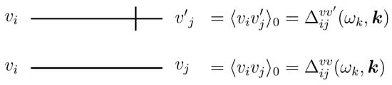
Figure 1.
Nontrivial propagators for the model in Equation (24).
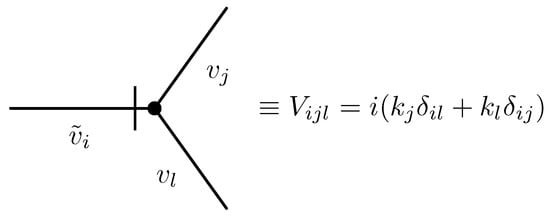
Figure 2.
Interaction vertex responsible for the nonlinear interactions between velocity fluctuations in the model in Equation (24). Momentum k on the right hand side corresponds to the inflowing momentum of the auxiliary field .
The theoretical description of the fluid turbulence on the basis of “first principles”, i.e., starting from the stochastic Navier–Stokes (NS) equation [25] remains an open problem. However, considerable progress has been made in understanding simplified model systems sharing certain essential properties with the real problem: stochastic Burgers equation [48], shell models [49] and advection by random “synthetic” velocity fields [33].
A paradigmatic model of a scalar quantity advected passively by a Gaussian random velocity field, uncorrelated in time and self-similar in space, the so-called Kraichnan’s rapid-change model [39], is a famous example. The standard notation for advection problem using the Kraichnan model slightly differs from the one using stochastic Navier–Stokes ensemble. Therefore, in what follows, we give a brief overview of basic physical ideas behind the Kraichnan model and introduce the corresponding notation.
The governing equation for diffusion–advection for field is
where is the coefficient of molecular diffusivity and is a zero-mean Gaussian random noise with the correlation function
The noise in Equation (33) maintains the steady-state of the system. The particular form of the correlator is not relevant, however. The sole condition which must be satisfied by the function is that it must fall off rapidly at . Here, L is an integral scale related to the stirring.
In accordance with the generalized Kraichnan model [34,50] with finite correlation time taken into account, we assume velocity field generated by a simple linear stochastic equation
where is a linear operation to be specified below and is a zero-mean random stirring force with the correlator
It should be noted that, in the SDE in Equation (33), the multiplicative noise due to random velocity is not a white noise in time as in the original Kraichnan model. Therefore, there is no need to specify the interpretation of the SDE. However, in the analysis, the white-noise limit is considered and it should recalled that in this limit the results correspond to the Stratonovich interpretation of the SDE in Equation (33).
The correlator is chosen [34,35,36] in the following form
with the wavenumber representation of the function :
The positive amplitude factors and are the coupling constants of the model. Furthermore, can be regarded as a formally small parameter of the perturbation theory. The positive exponents and () are RG expansion parameters. They are analogous to expansion parameter in the theory. Now, the expansion is carried out in the -plane around the origin .
Note the presence of two scales in the problem—integral scale L introduced in Equation (34) and momentum scale m, which has appeared in Equation (38). Clearly, they have different physical origins. However, these two scales can be related to each other and for technical purposes [35] it is reasonable to choose . When not explicitly stated, this relation is always assumed.
In the limit the functions in Equations (37) and (38) take on a simple powerlike form
which is convenient for actual calculations. The needed IR regularization will be given by restrictions on the region of integrations.
From Equations (35), (36) and (39), the statistics of the velocity field can be determined. It obeys Gaussian distribution with zero mean and correlator
where the kernel function is assumed in the form
The correlator in Equation (41) is directly connected to the energy spectrum via the frequency integral [34,51,52,53,54,55]
Hence, the coupling constant and the exponent characterize the equal-time velocity correlator or, similarly, energy spectrum. Further, the parameter and the exponent are related to the frequency (or to the function , the reciprocal of the correlation time at the wave number k) which describes the mode with wave number k [34,51,52,53,54,55,56,57]. Let us note that in the chosen notation the value corresponds to the well-known Kolmogorov “five-thirds law” for the spatial scaling behavior of the velocity field, and the value corresponds to the Kolmogorov frequency. A straightforward dimensional analysis reveals that the parameters (charges) and are connected to the ultraviolet (UV) momentum scale (of the same order of magnitude as the inverse Kolmogorov length) by the relations
In Ref. [50], it was demonstrated that the linear model in Equation (35) (and consequently the Gaussian model in Equation (40) as well) is not invariant under Galilean transformation and, therefore, it effectively neglects important effect of the self-advection of turbulent eddies. As a result of these so-called “sweeping effects” the different time correlations of the velocity are not self-similar and exhibit strong dependence on the integral scale [58,59,60,60]. However, the results presented in Ref. [50] lead to the conclusion that the Gaussian model describe the passive advection reasonably well in the appropriate frame of reference, in which the mean velocity field vanishes. An additional argument to support the model in Equation (40) is that we are mainly interested in the equal-time, Galilean invariant quantities (e.g., structure functions), which are not affected by the sweeping. Therefore, their absence in the Gaussian model in Equation (40) is not relevant [34,36,40].
The kernel function in Equation (41) is written in a very general form and allows studying various special limits, in which the numerical analysis of the resulting equations is simplified and which provide a deeper physical insight. Possible limiting cases are
- The rapid-change model corresponding to the limit . Then, the kernel function becomesThe velocity correlator is obviously —correlated in the time variable.
- The frozen velocity field arising in the limit , in which the kernel function corresponds to
- The purely potential velocity field obtained in the limit with constant. This case is similar to the model of random walks in a random environment with long-range correlations [61,62].
- The turbulent advection, for which . This choice mimics properties of the fully developed turbulence and yields well-known Kolmogorov scaling [23].
Using Equation (3), the stochastic problem in Equations (33)–(36) can be recast into the equivalent field theoretic model of the doubled set of fields with the action functional
where is defined in Equation (36), and as usual and are auxiliary response fields.
Generating functional of full Green functions is defined by Equation (7), where now a linear form is defined as
Following the argument in [34], we set in Equation (47) and carry out the explicit Gaussian integration over the auxiliary vector field, because we are not interested in the Green functions containing the auxiliary field . After the integration, we are left with the field-theoretic model with the action functional
where the second term represents the De Dominicis–Janssen action for the stochastic problem in Equation (33) at fixed velocity field . The first term describes the Gaussian averaging over specified by the correlator . The latter explicitly reads
The action in Equation (48) is written in a form that is suitable for a straightforward application of the field-theoretic perturbative analysis with the use of the standard Feynman diagrammatic technique. From the quadratic part of the action, we derive the matrix of bare propagators. The wavenumber frequency representations of relevant propagators are: (a) the bare propagator defined as follows
and (b) the bare propagator for the velocity field that reads
The triple (interaction) vertex can be rewritten in , where momentum is flowing into the vertex via the response field . A graphical representation of the perturbation elements for a Kraichnan-like model is schematically depicted in Figure 3.
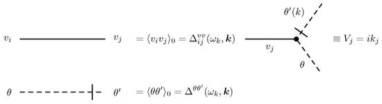
Figure 3.
Feynman rules for the model in Equation (48).
Taking as a example the Kraichnan model, let us briefly describe what kind of quantities might be studied by functional techniques. From experimental and theoretical point of view, the main focus is in the behavior of the equal-time structure functions
in the inertial range, specified by the inequalities (l is an internal length). Brackets denote the functional average over fields with the weight functional from Equation (48). In the isotropic case, the odd functions vanish identically, while for even functions a simple dimensional argument dictates the following form
where are scaling functions of purely dimensionless variables. In principle, functions can be calculated by means of the usual perturbation theory (i.e., as series in ). However, this is not a reasonable way to study the inertial-range behavior: the reason is that the coefficients are singular in the limits and/or and compensate for the smallness of . To obtain correct IR behavior the entire series have to be summed. Such a summation procedure can be effectively done by the use of the field theoretic RG and OPE (see Section 4 and Section 5).
The RG analysis can be divided into two stages. During the first stage, the multiplicative renormalizability of the model is proved and the differential RG equations for its correlation (structure) functions are derived. The asymptotic behavior of functions similar to the one in Equation (52) for and any fixed is governed by IR stable fixed points (see next section) of the RG equations and assumes the form
with so far unknown scaling functions . Whenever is a nonlinear function of N, we refer to such case as anomalous scaling or multiscaling.
Let us remind that the quantity is called the critical dimension. The exponent , the difference between the critical dimension and the canonical dimension , is known as the anomalous dimension. In the present case, the latter takes a simple form: . For any function , the representation in Equation (54) implies scaling behavior in the IR region (, fixed) with definite critical dimensions of all IR relevant parameters, , , and fixed irrelevant parameters and l.
In the second stage, the small behavior of the functions is analyzed in the general representation in Equation (54) employing the OPE technique (Section 5). It predicts that, in the limit , the functions have the asymptotic forms
where are coefficients regular in the variable . In general, the summation is performed over specific renormalized composite operators F with critical dimensions . Kraichnan model exhibits nontrivial scaling behavior as some of anomalous exponents are negative and singular behavior on L is present. Such situation never occurs in critical phenomena [5,6] where corresponding exponents are positive and lead only to subleading corrections.
More elaborated discussion on anomalous scaling can be found in Section 10, which is devoted to generalization of Kraichnan model. Namely, assumption of isotropy is abandoned and effect of anisotropy is taken into account.
4. Renormalization Group Analysis
Let us briefly summarize main ideas of the quantum-field theory of renormalization and RG technique; a detailed account can be found in monographs [5,6,15,46].
Feynman graphs of Green functions are a convenient graphical representation of perturbation theory. Quantum field theory models are well-known for appearance of UV divergences in loop diagrams. This results from an integration at large momenta. Therefore, it is necessary to find an effective procedure to eliminate these divergences step by step in a controlled manner. Finite diagrams (free of UV divergences) are brought by an iterative renormalization procedure. The inherent ambiguity of this removal of divergences may be used to establish connection between values of Green functions at different scales without having explicit solutions for them. This is the idea of the method of renormalization group (RG) proposed in the framework of high energy physics long time ago [1,7,8,9,10,11].
In statistical physics, RG allows one to extract relevant information about large-scale behavior from the mutual correlation between IR behavior of Green functions and UV divergences at critical dimension [5,15]. Thus, in statistical theories, the RG method can be understood as an effective way to determine non-trivial asymptotic behavior of Green functions in the range of small (infrared) wavevectors (scales).
There is simple criterion how to determine the true asymptotic range in the framework of the RG. One of the RG-functions is the -function, which is the coefficient of the operation in the RG equation. The -function is calculated perturbatively as infinite series of powers of the coupling constant g. Non-trivial asymptotic behavior is governed by RG fixed points , which are roots of the function (solutions of equation ). A fixed point can be IR or UV stable depending on the behavior of the -function in the vicinity of . Of course, physical theories contain usually many charges and these considerations have to be properly generalized [5,46].
The field theoretic RG is based on non-trivial techniques of UV renormalization. The basic procedure lies in a perturbative calculation of the RG-functions in the framework of a prescribed scheme of regularization [5,6]. To find and analyze UV divergences in a specific field-theoretic model counting of canonical scaling dimensions of fields and parameters of the model is used. The essence of such a power counting is closely connected with the existence of a scale invariance in the model.
For models considered in this paper, it is advantageous to calculate Feynman diagrams in a formal scheme [5] without UV-cut-off . Then, UV-divergences manifest themselves as poles in a dimensionless parameter that measures deviation from a logarithmic theory, i.e., a theory in which all coupling constants become dimensionless. The procedure of multiplicative renormalization removing UV-divergences (in the present case, poles in a parameter ) is the following: the original action is declared to be unrenormalized; its parameters (the letter stands for the whole set of parameters; for instance, coupling constants, deviation from criticality, viscosity, etc.) are the bare parameters, and they are assumed to be functions of the new renormalized parameters e. The new renormalized action is the functional with certain (to be determined perturbatively such that the Green functions generated by the renormalized action are UV finite, i.e., regular in ) renormalization constants of fields (one per each independent component of the field) and parameters . In unrenormalized full Green functions , the functional averaging is performed with the weight functional , whereas, in renormalized functions , with the renormalized weight functional . The relation between the functionals and leads to the relation between the corresponding Green functions , where by definition (ellipsis denotes other arguments such as coordinates or wavenumbers), and, by convention, the quantities and are expressed in terms of the parameters e. The correspondence within perturbation theory is assumed to be one-to-one, therefore either of the sets can be taken as the independent variables.
For translationally invariant theories, it is much more convenient to deal not with the full Green functions , but with their connected parts . Their generating functional being through the relation
A further simplification is possible through 1-irreducible functions (also called one particle irreducible functions or vertex functions). The generating functional for the latter is defined by the functional Legendre transform [47]
where
To simplify notation in practical calculations, it is convenient to relabel -variables back to the original fields . This allows us to rewrite the first relation in Equation (57) compactly as
where is the sum of all one particle irreducible (1PI) loop diagrams [5].
Statements of RG theory are readily summarized at the level of corresponding Green functions. For connected and 1PI Green functions, they read
where the functions can be chosen arbitrarily, which implies an arbitrary choice of normalization of the fields and parameters e at given . In the present text, we also interchangeably use the following notation for the connected Green functions
and for the 1PI Green functions according to the aforementioned relabeling
The crucial statement of the theory of renormalization is that for the multiplicatively renormalizable models these functions can be chosen to provide UV finiteness of Green functions as With this choice, all UV divergences (poles in ) contained in the functions are absent in renormalized Green functions . We note that the UV finiteness in this sense of any one set of Green functions (full, connected, and 1-irreducible) automatically leads to the UV-finiteness of any other. The RG equations are written for the renormalized functions which differ from the original unrenormalized functions only by normalization, and, therefore, can be used equally well to analyze the critical scaling. Let us recall an elementary derivation of the RG equations [5,46]. The requirement of elimination of divergences does not uniquely determine the functions and . An arbitrariness remains which allows introducing an additional dimensional parameter scale setting parameter (renormalization mass) in these functions (and via them also into )
A change of at fixed leads to a change of and for unchanged . We denote by the differential operator for fixed and apply it to both sides of the equation with it. This yields the basic RG differential equation
where the operator is expressed in the variables The coefficients and are called the RG functions and are calculated in terms of various renormalization constants Z. Coupling constants (charges) g are those parameters e, on which the renormalization constants depend. Logarithmic derivatives of charges in Equation (65) are functions
All the RG-functions are UV-finite, i.e., have no poles in , which is a consequence of the functions being UV-finite in Equation (65).
For models considered in the present work, the analysis of divergences should be augmented by the following considerations:
- For any dynamic model in Equation (1), all 1PI Green functions containing only the original fields are proportional to the closed loops of step functions, hence they vanish, and thus do not generate counterterms.
- If for some reason several external momenta or frequencies occur as an overall factor in all the Feynman diagrams of a particular Green function, the real degree of divergence is less than by the corresponding number of units.
- Sometimes the divergences formally allowed by dimensionality are absent due to symmetry restrictions, for instance, the Galilean invariance of the fully developed turbulence [31] restricts the form of possible counterterms.
- Nonlocal terms of the model are not renormalized.
In principle, these general considerations permit determining all superficially divergent functions and to explicitly obtain the corresponding counter-terms for any dynamic model.
The most convenient scheme for analytic calculations is the scheme of minimal subtractions (MS) proposed in [63], in which all the renormalization constants Z in the perturbation theory are of the form
In the dimensional renormalization the contribution to the coefficient of in Equation (67) may be expressed as a Laurent series in . In the MS scheme, only the singular part of the Laurent expansion of each coefficient is retained. In any other renormalization scheme, the renormalization constant is of the form
where the regular part of each coefficient is, by and large, an arbitrary regular function of at the origin.
5. Composite Operators and Operator Product Expansion
In this section, we recall the basic information about renormalization and critical exponents (dimensions) of composite operators, i.e., local products of the basic fields of the model and their derivatives. In the models we are interested in, they are constructed from the velocity field scalar field or magnetic field at the single space-time point . Examples are , and so on.
A theoretical analysis of composite operators and their renormalization is important at least for two reasons. First, their critical dimensions and correlation functions can be measured experimentally and for some operators such data are available [64,65]. For instance, in the fully developed turbulence, the mean of the energy dissipation is proportional to the statistical average of the composite operator . This quantity enters the equation of energy balance and contributes to the redistribution of the energy of the turbulent motion and its dissipation. Moreover, strong statistical fluctuations of the operator of energy dissipation seem to account for deviations from Kolmogorov’s exponents and lead to the intermittency (multifractality) of the turbulent processes [23]. Second, the general solution of the RG equation (Equation (65)) contains an unknown scaling function depending on dimensionless effective variables (coupling constants, viscosity, etc.). This function can be calculated in the framework of usual perturbation scheme in an expansion parameter but, as mentioned above, in certain asymptotic ranges of scales, this calculation fails. Both experimental and theoretical reasons in theory of turbulence motivate us to study behavior of correlation functions with respect to outer (integral) scale L. Let us elucidate this issue in some detail. As an example we consider pair correlation function for velocity fluctuations for field-theoretic model in Equation (24). There is no field renormalization in this model [32], therefore the Green function coincide with the unrenormalized function The only difference lies in a choice of variable and perturbation theory (expansion either in charge g or , respectively). In renormalized variable correlation, function depends on and L. From a dimensional consideration, we directly see that can be represented in the form
where R is a function of dimensionless parameters and for brevity we have not explicitly written the transverse projection operator. The correlation function satisfies a general RG equation with , which is a direct consequence of absence of renormalization of velocity field , and reads
The solution of this equation can be found using the method of characteristics and presented in the form
where are invariant variables, i.e., the first integrals of Equation (70). Using standard RG considerations, the invariant viscosity [31] takes the following form
As the parameter s approaches zero, invariant charge approaches IR fixed point and . Hence, at fixed point (far from dissipation scales ), the single-time correlation function of velocity field takes the scaling form
Setting gives kinetic energy spectrum that behaves as a power-law function of wavevector k. This coincides with Kolmogorov’s prediction for the exponent. The remaining scaling function R is not determined yet and in general it is possible to employ perturbation theory and obtain infinite series in parameter . In particular, in the theory of turbulence, the main interest is in the scaling function in the inertial interval . In the theory of critical phenomena, the asymptotic form of scaling functions for (formally, ) is studied using Wilson’s operator product expansion (OPE) (see, e.g., [6,66]). The analog of L in turbulence is played by the correlation length in critical phenomena. It turns out that this technique can be used also in the theory of turbulence and in simplified (toy) models associated with the genuine turbulence (see, e.g., [5,31,33,67,68]).
The generating functional of the correlation functions of the field with one insertion of the composite operator has the form (compare with the generating functional in Equation (7) for the usual correlation functions of )
Since the arguments of the fields in the operator F coincide (giving rise to new closed loops in the Feynman diagrams), correlation functions with these operators contain new UV divergences, which have to removed by an additional renormalization procedure (see, e.g., [5,6,66]). The standard RG equations yield the IR scaling of the renormalized correlation functions with definite critical dimensions of a set of basis operators F. Due to the renormalization, is not the sum of critical dimensions of the fields and derivatives in F. A detailed analysis of the renormalization procedure of composite operators for the stochastic NS problem can be found in the review [67], and below we restrict ourselves to the necessary information only.
As a rule, composite operators are mixed during the renormalization procedure, i.e., an UV finite renormalized operator (correlation functions with one insertion of do not possess UV divergences) takes the form counterterms, in which “counterterms” stands for a linear combination of the operator F itself and other unrenormalized operators mixing the the operator F. Let denote a closed set of operators mixing only with each other under renormalization. For this set, the matrix of renormalization constants and the matrix of anomalous dimensions are defined by
The subsequent matrix of critical dimensions reads
in which , , and denote diagonal matrices of canonical dimensions of the operators of the closed set (the diagonal element corresponding to a particular operator F is equal to the sum of canonical dimensions of all fields, their derivatives and renormalized parameters in F) and is the matrix in Equation (75) at the fixed point.
Critical dimensions of the set correspond to the eigenvalues of the matrix . The basis operators possessing definite critical dimensions are linear combinations of the renormalized operators
where the matrix is such that the matrix is diagonal.
Counterterms generated by a given operator F are determined by all possible 1PI Green functions with one insertion of operator F and an arbitrary number of primary fields ,
The total canonical dimension (the formal degree of divergence) for these functions is given by
where the sum is taken over all types of field arguments. For is a nonnegative integer.
According to the OPE, the single-time product of two renormalized operators at , and can be represented as follows
Here, the functions are the Wilson coefficients regular in L, whereas are all possible renormalized local composite operators of the type in Equation (77) allowed by symmetry arguments, with specific critical dimensions .
The renormalized correlator is obtained by averaging Equation (80) with the weight , quantities involving dimensionless (scaling) functions appear on the right hand side. Their asymptotic behavior for is found from the corresponding RG equations (see [34] for the case of Kraichnan model) and has the form
From the operator product expansion in Equation (80), we therefore get
where the quantities generated by the Wilson coefficients in Equation (80) are regular in L, the summation is carried out over all possible composite renormalized basis operators allowed by the symmetry of the left side, and are their critical dimensions. The leading contributions for are those with the least dimension In the theory of critical phenomena, it is observed that all the nontrivial composite operators have positive critical dimensions for small and the most important term in Equation (82) corresponds to the simplest operator with , i.e., the function is finite as (see [6]). However, as has been noted in [68] in the model of developed turbulence composite operators with negative critical dimensions exist and are responsible for possible singular behavior of the scaling functions such as N-point correlation functions as . We call operators with —if they exist—dangerous [67]. This is motivated by the fact that they correspond to contributions to Equation (82) which diverge for . The scaling functions in Equation (82) decomposed in dangerous operators exhibit anomalous scaling behavior which is a manifestation of a nontrivial multifractal (intermittent) nature of the statistical fluctuations of the random fields under consideration and globally all the physical system.
Dangerous composite operators in the stochastic model of turbulence occur only for finite values of the RG expansion parameter . Let us note that within the expansion it is not possible to determine whether or not a given operator is dangerous, if only its critical dimension is not found exactly employing the Schwinger equations, etc. or the Galilean symmetry (see [67,69]). Furthermore, dangerous operators appear in the operator product expansion in the form of infinite families with the spectrum of critical dimensions unbounded from below. Therefore, for a proper analysis of the large L behavior, a summation of their contributions is called for.
6. Schwinger Equations and Conservation Laws
Useful information about composite operators can be gained even without an actual calculation of Feynman diagrams. Exploiting invariance properties of functional integrals provides nontrivial relations known as Schwinger equations [47]. One of the simplest symmetries is the translation invariance of action in Equation (3). It is invariance with respect to a shift , where is a suitably chosen function that vanishes sufficiently fast, i.e., . Such translations do not change the integration measure and as a result the quantity does not depend on for any functional . We then easily derive that the first variation with respect to yields a formal relation
written in the notation of Equation (7). The following relation is of particular importance
Performing variational derivatives gives us
Multiplication by field inside the functional integral is tantamount to a differentiation with respect to the corresponding source field A. This observation allows us to rewrite Equation (85)
Substituting , we obtain the corresponding Schwinger equation for where from we can derive the equation for All these equations are of finite order (for polynomial action) in functional derivatives, and each of them is tantamount to an infinite chain of connected equations for the Green functions—the expansion coefficients of the corresponding functionals [47].
In the following discussion, we need one additional relation that corresponds to the Schwinger equation
where stands for either the fluctuating field or the corresponding response field.
As discussed in Section 5, composite operators are related to experimentally measurable physical quantities. We illustrate this claim on an example of stochastic hydrodynamics summarized in the field-theoretic action in Equation (24). Our aim is to elucidate transfer of energy in a stationary of turbulent state. The latter condition ensures that time derivatives of averaged quantities are identically zero.
Let us derive equations describing energy and momentum transfer in turbulent flows. To obtain an equation expressing momentum conservation, we employ the first equation in Equation (87), where consists of altogether two d-dimensional vector fields . First, for , we choose a response field , and we get
Performing indicated derivative, we obtain differential equation
Due to transversality of response field , a nonlocal term has appeared, which corresponds to the pressure fluctuations
To derive an equation describing energy transfer, we utilize the second Schwinger equation (Equation (87)). In particular, letting and in Equation (87) yields
In an analogous manner to Equation (89), we get
written in a component notation. Note that all quantities have been normalized to unit mass, i.e., density has been set to unity (). Equations (89) and (92) represent conservation laws for momentum and energy. They can be further rewritten into a physically more transparent form
where might be interpreted as momentum density, is energy density, is tensor of momentum transfer, is vector of energy flow, and is a rate of energy dissipation. Direct comparison of Equations (89) and (92) with Equations (93) and (94) yields explicit expressions
We recognize Equation (93) as a stochastic Navier–Stokes equation stirred by random force and regular force .
Functional averaging of Equations (93) and (94) according to the prescription in Equation (6) with weigh functional leads to the balance equation for energy and momentum. Assuming vanishing external force , we obtain the following equation for time derivative of energy
It is clear that for homogeneous and isotropic flows at zero external force the mean value of an arbitrary composite operator could not depend on the position . Hence, it is constant and consequently all spatial derivatives are identically zero. From Equation (98), we then get for steady state
where we have introduced the following abbreviation for mean energy dissipation
Let us recall (see Equation (19)) that pair correlation for random force can be written as Insertion of this relation into Equation (100) and integrating over time variable t yields
To the lowest order in perturbation theory, the retarded response function is -correlated in spatial variable. This property holds also for the full response function (what follows from a straightforward analysis of Feynman graphs) and therefore
Insertion of this relation into Equation (101), recalling Equation (20) and integrating through spatial variable , we derive
Summation over internal indices i and j corresponds to a calculation for a trace of transverse projection operator , which equals . Thus, we finally arrive at the expression
This relation reflects an important property of stationary homogeneous turbulence. It expresses the expected fact that, to achieve a stationary state, it is necessary to inject energy into a system in a continuous fashion. In the stochastic approach, this is done through a random force, which compensates energetic losses due to friction processes. These losses are expressed through mean energy dissipation .
7. Ward Identities and Galilean Invariance
We say that a given theory possesses a symmetry, if the corresponding action functional of the theory is zero under the action generating this symmetry. Ward–Takahashi identities mathematically express inherent symmetry of a given field-theoretic action. In stochastic models of turbulence, they correspond to the well-known Galilean invariance. As a rule, these identities provide nontrivial relations between various Green functions of theory and consequently between renormalization constants. Moreover, they are also relevant for an analysis of composite operators.
As pointed out in Section 4, certain divergences present in Feynman diagrams of the perturbative expansion of a Green function might cancel each other, so that the given Green function is in fact UV finite. This compensation might be caused by the inherent fact that the underlying stochastic model describing developed turbulence is invariant with respect to the Galilean transformations. Of course, such and similar mechanisms are quite general in physics. As a further example, we can mention absence of potential UV divergences in quantum electrodynamics, or even quantum chromodynamics describing strong interactions between quarks and gluons. The underlying symmetry in these cases is gauge symmetry.
Now, we show that Galilean invariance in the model in Equation (24) ensures that UV divergences in triple 1PI function
are actually absent. The essential idea consists in a derivation of certain Ward identity, which takes form of an differential equation relating the triple 1PI Green function with the pair 1PI Green function , which is an abbreviation for
These relations stem from invariance property of generating functional with respect to the Galilean transformations. Then, an absence of certain types of UV divergences in leads to absence of divergences in .
Let us consider a generalized Galilean transformation of fields defined as follows
where
Here, is some velocity vector describing the Galilean transformation. The spatial vector is responsible for a shift of spatial coordinate . The transformations in Equation (107) are a generalization of the standard Galilean transformations [70], in which velocity is constant in time variable. This is brought about by functional integration in which functional space has to be restricted by appropriate conditions. Here, it is required that velocity and response fields and vanish sufficiently quickly in the limit . Of course, arbitrary symmetry transformation of the model must comply with this property.
Insertion of Equation (107) into the action in Equation (24) yields the following relation for the transformed action
where in the last equation we have transformed time derivative using partial integration. In this derivation, the following relations for variational derivatives have been utilized
which can be directly obtained from Equation (107). In infinitesimal form, Equation (109) takes form
where
The implicit assumption in derivation of Equation (113) is smallness of velocity .
In a compact form, the requirement of Galilean invariance for the model in Equation (24) is equivalent to the condition
or in an infinitesimal form
The Ward identities are useful not only for Green functions of basic fields , but for composite operators as well (see Section 5). This motivates an introduction of generalized generating functional that includes composite operators F. It can be presented in the following form
where stands for . Sources correspond to N composite operators . In principle, the functional in Equation (117) generates not only all possible Green functions of basic fields, but also full Green functions consisting of arbitrary inclusion of composite operators and fields. In this regard, it is useful to compare this generating functional in Equation (117) with the functional in Equation (74) that generates Green functions containing one inclusion of composite operator F.
The functional measure is obviously translationally invariant. Hence, equality is satisfied and Equation (116) can be rewritten in the following way
or
As source fields A and a are independent, the choice yields Ward identities for Green functions of basic fields, whereas leads to additional Ward identities for Green functions containing contributions from composite operators. Further, we concentrate on derivation of Ward identity for Green function containing solely basic fields , which we derive from Equation (119) inserting . We have
where double brackets correspond to the functional averaging with respect to the weight functional
Using the relations in Equations (108)–(111), we rewrite Equation (120) in the component notation
where for brevity we have denoted , , and . As Galilean velocity is arbitrary, Equation (122) can be further simplified to
Every term in Equation (123) containing fields might be obtained by taking an appropriate number of derivatives of with respect to source A. This means that field can be effectively replaced by variational derivative
Hence, we get
In this formulation, the whole expression in brackets does not depend on integration over fields and the equation can be further rewritten in terms of generating functional
Substituting , we rewrite Equation (126) into equation for generating functional for connected Green functions
Finally, by means of the functional Legendre transformations in Equation (57), we rewrite Equation (127) in terms of generating functional for 1PI (vertex) functions
where
Generating functional can be represented in form of formal Taylor series with respect to sources , in which coefficients by powers () are 1PI Green functions. The first few terms are
where, for instance, the second term actually stands for an expression
Insertion of this expansion into Equation (128), we get an infinite system of the Ward identities that relates various 1PI Green functions. For the present discussion, the most relevant is the Ward identity between pair (two-point) and triple (three-point) Green functions. The substitution of the expansion in Equation (130) into Equation (128) yields a formal polynomial in variables and . A comparison of terms proportional to term gives the following relation
Due to translation, invariance, , therefore
Let us integrate the second term in this equation over time t ( does not depend on time variable t, only on and ). It is straightforward to show that
Employing this relation in Equation (134), we finally obtain the required Ward identity in the coordinate representation
For an analysis of UV divergences, it is useful to rewrite the Ward identity into a frequency– momentum (Fourier) representation. Let us determine Fourier transforms of pair and triple Green functions. They read
where . Translation invariance in time and space variables dictates
This allows us to simplify Equation (137) into
A similar consideration applies also for the triple Green function and leads to the Fourier representation
Hence, we derive
Insertion of the relations in Equations (139) and (141) into Equation (136) leads to the Ward identity in form
This relation can be conveniently represented in a graphical form as follows

From the Ward identity, it directly follows that there are no UV divergences in triple Green functions. In fact, on the right hand side of Equation (143), we have the Green function which contains only divergent structures that are proportional to (divergences proportional to frequency ). Therefore, taking derivative with respect to frequency ensures that the divergent part on right hand side of Equation (143) vanishes. Hence, the right hand side of Equation (143) is UV finite and therefore also the left hand side of the given equation is UV finite. This concludes the proof of UV finiteness of the triple one-time 1PI Green function .
8. Symmetry Restoration
In the previous Section 7, we show that the Galilean symmetry in Equations (107) and (108) restricts appearances of UV divergences in the perturbation theory. In this regard, a natural question arises: What can violation of the Galilean symmetry lead to? We address this issue in the context of the stochastic Navier–Stokes model in Equation (24). Let us note that the following exposition closely follows that in [71], where all necessary technical details can be found. Violation can be achieved by various means. In particular, it can be achieved by modification of time behavior of the force correlator in Equation (20). Let us imagine that there exists microscopic finite correlation time behaving according to Ornstein-Uhlenbeck process [17,72].
Without loss of generality, let us consider a generalization of Equation (23) as
where the kernel function now assumes the following form
Exponent is related to the dispersion law . From dimensional considerations, parameter can be represented as
which can be interpreted as a defining relation for charge . Quite general form of Equation (145) allows studying two special cases: the limit fully corresponds to the time-independent correlation of random force. On the other hand, the limit yields the previously analyzed Galilean model in Equation (20).
The propagator in the frequency–momentum representation takes the form
According to the theoretical consideration discussed in Section 2 and Section 4, it can be shown [71] that the model corresponding to Equation (24) with Equation (145) is multiplicatively renormalizable in which two renormalization constants and have to be added. The renormalized action functional is
where g, , and u are the renormalized counterparts of the bare (original) parameters; the correlation function is written in terms of the renormalized parameters with the use of the relation ; and the reference scale is a new free parameter of the renormalized model. The action of the renormalized model in Equation (148) can be constructed from the original action in Equation (24) by renormalization of fields , and parameters
The leading one-loop calculation [71] of Feynman diagrams is relatively straightforward and ensuing anomalous dimensions are
where for brevity the following redefinition of the charge g
has been used. Further, from the relations in Equation (150), we get -functions
A straightforward analysis of the functions reveals three IR fixed points: the trivial fixed point (zero values of charges’ coordinates) and two nontrivial fixed points. The trivial (Gaussian) fixed point, at which all nonlinearities are IR irrelevant, is
and is IR attractive when both y and are negative.
A further fixed point with the coordinates
is actually of a saddle-point type for, which one eigenvalue of the matrix is positive and the other negative.
The most interesting fixed point is actually obtained in the limit , from Equations (145) and (147). This case corresponds to an earlier studied model with random force uncorrelated in time [32]. Therefore, we might expect to find the known fixed point of this model. Introducing a new variable , one obtains a new function of the following form
Actual calculations reveal the existence of the fixed point with the coordinates
which coincides with that in Ref. [32] and is IR attractive in the region restricted by inequalities and .
The main conclusion from these considerations is that at the only nontrivial IR attractive fixed point correlation time vanishes. In other words, the Galilean symmetry, broken by the colored random force in Equation (145), is reestablished in the IR limit.
9. Parity Breaking in Magnetohydrodynamic Turbulence
In addition to the passive scalar problems introduced in Section 3, there exists a broad class of problems related to vector admixtures [23,35]. Due to the presence of more degrees of freedom, it is natural to expect that observed behavior can be richer than in scalar case. Among many, much attraction has been gained by a model of magnetohydrodynamics (MHD) [73,74,75,76]. The interplay between the velocity field and the magnetic field is crucial in explaining many phenomena—magnetic dynamo, convective processes, galaxy formation, etc. [77,78,79,80,81]—therefore it is clear that it has to be taken into account properly.
The full stochastic MHD problem is rather complicated, therefore for many purposes for a theoretical description it has been proposed to use a simplified model—the kinematic Kazantsev– Kraichnan model [35]. Its basic assumption is that the vector field of magnetic induction (hereinafter, referred to as vector) is passively advected by the turbulent flow, but reaction on the velocity field by the magnetic field is neglected. The most notable point of criticism to the Kazantsev–Kraichnan model is the assumption about the velocity field using a simple Gaussian statistical ensemble. From a more fundamental point of view, the velocity field would be generated dynamically. Therefore, we assume here that the velocity field is brought about by the stochastic Navier–Stokes equation expounded in Section 3.
The introduction of magnetic field in the Kazantsev–Kraichnan model comes from a physical approximation called magnetohydrodynamic limit [74,75]. It is assumed that the matter is electrically neutral at large scales and that the mean free path is much shorter than the corresponding Debye length. This assures that the electric displacement field accounting for the overall motion of charged particles can be entirely neglected. The system is then completely described in terms of the variables of density, pressure, and mean velocity field. From the RG point of view the displacement field is IR irrelevant. Hence, there is no need to retain it. Faraday’s law together with the generalized Ohm’s law give rise to the advection–diffusion equation . According to the functional formulation from Section 2, the corresponding stochastic problem assumes the form
where is just the fluctuating component of the magnetic induction, is the magnetic diffusion coefficient, and a stochastic source term has been added to the right side. This term is the random part of the curl of the current and stems from the intrinsic randomness of the magnetic field [31]. A detailed account of the MHD problem can be found in [73,74,75].
The random source in Equation (158) is assumed to be zero-mean Gaussian with the correlation function
where is a function, whose exact form is irrelevant. It must have a finite limit at and vanish at . The magnetic field is solenoidal, therefore the terms and are equal.
In realistic scenarios, the stochastic NS equation (Equation (16)) has to be amended by a Lorentz term responsible for the backward influence of the magnetic field on the velocity field. This is brought about by a familiar force term in conducting fluid of form . The most important consequence of this argument is an important physical effect known as the turbulent dynamo: generation of magnetic field at large scales by the turbulent motion. Let us make an important remark, which should clarify the fundamental difference between equilibrium statistical models and non-equilibrium ones. The turbulent dynamo might be explained by the mechanism of spontaneous symmetry breaking most spectacularly associated with the Higgs mechanism in particle physics. Here, “the ground state” of the turbulent gyrotropic fluid with vanishing mean of the magnetic field is unstable. It is stabilized by the spontaneous generation of a spatially uniform anomalous mean . This happens in full analogy with the situation in a ferromagnetic material below , in which magnetic order is stabilized by the appearance of spontaneous magnetization. The condition for total magnetization follows from an extremal condition imposed on free energy. On the other hand, for the dynamo problem, the resulting field is determined by the properties of the response function. In particular, it is required that all perturbations from a given stable state have to be damped out sufficiently quickly. Let us note that that the instability manifests itself not at the level of the action function but only at the following one-loop approximation.
Let us discuss the full MHD problem in more detail and introduce one specific generalization. From now on, we assume that the MHD problem is governed by two coupled equations [22]
where denotes a solenoidal vector field advected by a helical turbulent flow of an incompressible velocity field . Both fields and are divergenceless. In other words, they satisfy the incompressibility condition
Further, is the bare inverse Prandtl number [23,26]. Functions and in Equations (160) and (161) representing pressure fields are not relevant in the following analysis. In fact, due to the solenoidal property in Equation (162), functions P and Q can be expressed in terms of a formal Biot–Savart law [23,26]. A is a dimensionless parameter of the model. Three particular values of the parameter A have been analyzed in detail [35]. First, the value yields the Kazantsev–Kraichnan kinematic dynamo model, where the pressure term in Equation (161) drops out. Second, the choice leads to the model of passively advected vector admixture. Third, the value corresponds to the linearized NS equation in a background field with given statistics. It is therefore convenient to retain A as a free parameter and analyze all three models together. The model in Equation (161) is often called the generic A model in the literature [35,82,83]. The complete model thus comprises two interconnected stochastic equations (Equations (160) and (161)).
Stochastic random sources and must be included in the coarse-grained setup of turbulence and MHD problems. As usual, it is assumed that the random variable is Gaussian with zero mean and correlation function
Here, L is the integral scale of stirring of the magnetic field , is finite at and at it should rapidly fall off. Apart from these restrictions, needs not be specified [35]. Further, mimics the pumping of kinetic energy in the system at the largest spatial scales and is subject to the condition of real IR energy injection implemented through its specific power-like form suited to the RG approach [5]. However, the results obtained do not depend on specific forcing statistics because of the universality of fully developed turbulence. Hence, we only take advantage of the most suitable forcing in the RG analysis. Following this standard argument [5], we choose the pair correlation function of zero-mean Gaussian statistics
where denotes the space dimension; is the wavevector with the magnitude ; and is the positive quantity, where is a coupling constant connected to the typical UV momentum scale through . The parameter specifies the power-like behavior of the energy pumping at large scales and assumes the value of 2 in the physically relevant IR energy pumping. In the RG analysis of the fully developed turbulence, is assumed small in calculations. Its physical value of 2 is inserted into perturbative expansions only as the last step [5]. The tensor quantity determines the spatial parity violation in the model at hand. In symmetric isotropic incompressible turbulent fluid, such as analyzed here, the tensor corresponds to the sum of the ordinary transverse projection operator and a helical term , i.e.,
where is the third-rank completely antisymmetric tensor. The real-valued helicity parameter obeys the inequality dictated by the condition that the correlation function is positive definite in Equation (164). Evidently, the value corresponds to the isotropic (non-helical) case, while the value corresponds to fully broken spatial parity.
Following the De Dominicis–Janssen approach (Section 2), the stochastic problem of Equations (160) and (161) is equivalent to a field-theoretic model with the set of fields , where the fields with primes once more denote the response fields [5,45]. Thus, the field-theoretic model is given by the Dominicis–Janssen action
where and are defined in Equations (163) and (164), respectively. As usual, summations over repeated indices are implied. As the original fields and , the response fields are solenoidal, i.e., . In the frequency–momentum representation, free propagators of the model in Equation (166) are
The function is the Fourier transform of the function introduced in Equation (163). Moreover, the theory includes three interaction vertices
- : ,
- :
- :
In the momentum–frequency representation, they are associated with the vertex factors [5]
In all these vertices, momentum is flowing into through the corresponding response field, i.e., in it is the response field and in the field . A graphical representation of interaction vertices is displayed in Figure 4.
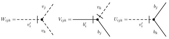
Figure 4.
Graphical representation of all interaction vertices of the model related velocity non-linearities of the action (166).
The field theoretic model defined by the action in Equation (166) is intrinsically unstable due to the fact that 1PI graphs and are not UV finite. To ensure the stabilization of the advection–diffusion system, we assume—inspired by the argument in [84]—that the vector field fluctuates around a spontaneously generated non-vanishing mean with the magnitude depending on the parameter A. The auxiliary field is still supposed to have vanishing mean. Technically, the spontaneous symmetry breaking is achieved by the substitution of the sum instead of the vector field in the action in Equation (166). Such a change of variables gives rise to a new action functional with the free part now containing additional terms, whereas the interacting part remains intact. The action functional with broken symmetry is
The quadratic part of this action determines propagators of the theory and now it has more involved structure than Equation (166). It is seen that the symmetry breaking brings about cross propagators , , , and . Furthermore, all propagators are more complicated and depend on the uniform magnetic field explicitly. In the frequency–momentum representation, they are
Here, following abbreviations have been introduced
for brevity. Propagators are depicted in Figure 5.

Figure 5.
Graphical representation of all propagators of the model given by the quadratic part of the action (166).
Identification of all relevant UV divergences is carried out by the standard power counting. We omit the details, which are analogous to those in Ref. [82]. The model at hand is logarithmic at . In the framework of the minimal subtraction (MS) scheme, this means that all possible UV divergences are poles in [5]. Following the analysis of Hnatič and Zalom [82], we arrive at the conclusion that all UV divergences are absorbed in counterterms and . Thus, the model is multiplicatively renormalizable with renormalized parameters , , and
where , and are the corresponding renormalized parameters. The renormalization mass is introduced as a consequence of the analytic regularization used in calculations. The quantities contain poles in the exponent . The renormalized action functional can be written as follows
where and are renormalization constants defined by relations
Both renormalization constants, and , correspond to a different class of Feynman diagrams (details below). However, they reveal a common structure in the MS scheme: the nth order of perturbation theory is related to the nth power of g with the corresponding coefficient containing poles in of order n and less [5].
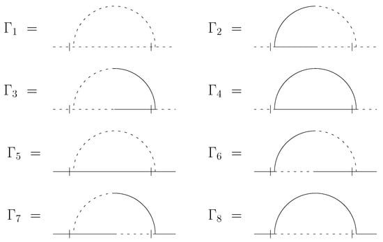
Figure 6.
Graphical representation of all Feynman diagrams for two-point one-irreducible Green functions of the action (176). Graphs represent perturbation expansion for function, and for function.
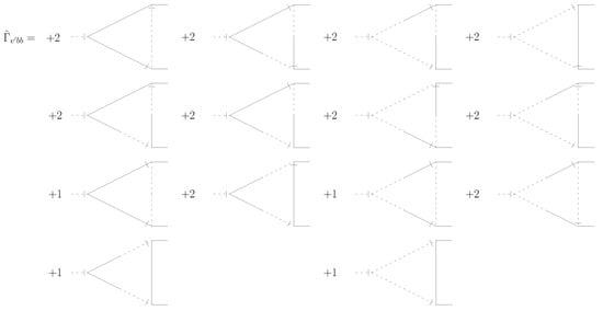
Figure 7.
Graphical representation of all one-loop Feynman diagrams forces for one-irreducible Green function .
One-loop calculation [84] of self-energy graphs for the 1PI function yields the following expression
where
Here, are components of the unit vector pointing in the direction of the spontaneous magnetic field. Terms proportional to might in principle generate instabilities. In the literature, the term proportional to is known as exotic. As detailed analysis [84] shows, terms can be eliminated by imposing the following relation
where the parameter A should not be equal to 0 or . At real space dimension , we get
To get insight into relevance of the last term on the right hand side of Equation (179), let us consider the approximate case of linearized MHD equations in polarized medium
where for brevity we have denoted , introduced as notation for certain combination of model parameters and employed the time–momentum representation [84]. Solution is sought in the form of plane waves
For an inviscid medium () without the exotic term (), we get a solution known as Alfvén waves for which
The solution with the exotic term is more complicated. To find solutions with the exotic term (), let us first find a convenient orthonormal basis of three vectors . The following choice
turns out to be case and qualitatively is depicted in Figure 8.
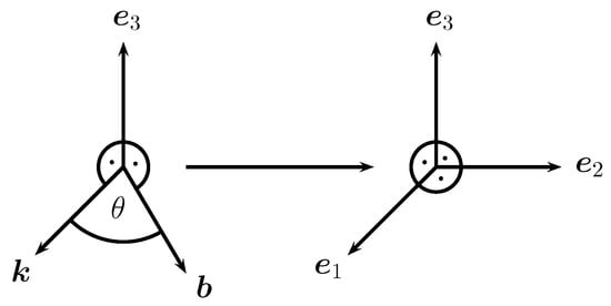
Figure 8.
Construction of the proper orthonormal basis for a sought solution of linearized MHD equations.
The transverse velocity and magnetic vector fields are perpendicular to the wavevector or, equivalently, to the basis vector . Let us decompose fields into perpendicular components and as follows
It is a straightforward exercise to check that modes satisfy following equations
Solution of these equations can be represented in the form
Thus, field-theoretic methods not only explain the emergence of turbulent dynamo, but also lead to an accompanying physical effect: appearance of disturbances in Alfvén waves perpendicular to the spontaneous field , which leads to their linear growth in time. This generates long-lived pulses —similar to Goldstone bosons.
An intriguing unsolved problem remains, however. Although gyrotropy is the cause of the dynamo effect, the value in Equation (180) calculated for the spontaneous magnetic field is independent of the parameter . Thus, any however small gyrotropy causes emergence of a finite spontaneous field. It is thus not clear whether or not the dynamo will also occur in a normal fluid in which .
10. Effect of Strong Anisotropy
Another related problem that can be addressed is the effect of large-scale anisotropy on statistics of the velocity field, and the passively advected fields in the inertial range [34,36,85,86,87,88,89,90,91,92,93,94,95,96,97,98,99]. The classical Kolmogorov–Obukhov theory predicts that the anisotropy generated at large spatial scales by the forcing (boundary conditions, geometry of the mesh, etc.) fades away when the energy is transferred down to the smaller scales by means of the cascade mechanism [23,25]. This picture is corroborated in recent analyses for even correlation functions. Thus, they provide us with some backup to the hypothesis of the restored local isotropy of the turbulence for the velocity field and passively advected field in the inertial range [34,36,90,91,92,93,94,95,97,98,99]. More specifically, the exponents describing the scaling in the inertial range exhibit universality and hierarchy related to the state of anisotropy. In particular, the main contribution to an even function comes from the exponent from the isotropic shell [34,36,89,91,92,93,94,97,98,99]. However, the anisotropy survives in the inertial range being explicit in odd correlation functions. This is inconsistent with the behavior anticipated on grounds of the cascade picture. Further, the skewness factor decreases with the length scale much more slowly than expected [50,85,86,87,88,100,101,102,103], whereas the odd dimensionless ratios of structure functions of higher order (hyperskewness, etc.) increase. This hints at persistent anisotropy at small scales [34,36,90,92]. This appears a universal effect as it is observed for both the scalar [34,36] and vector [92] fields, advected by the Gaussian rapid-change velocity, as well as for the scalar advected by the two-dimensional velocity field generated by the stochastic Navier–Stokes equation [90].
Here, we demonstrate the anomalous scaling behavior of a passive scalar advected by the velocity field due to the Kraichnan model with strong anisotropy. In contrast with the studies in [34,36,50,85,86,87,88,103], where the velocity field was assumed isotropic and the anisotropy was generated at large scales by the imposed linear mean gradient, the uniaxial anisotropy in considered model is present at all scales. The anomalous exponents turn out to depend on the anisotropy parameters and are thus not universal.
The aim of this section is twofold. First, expressions for the structure functions and correlation functions of the scalar gradients are obtained and then the corresponding anomalous exponents are computed in the leading order of the expansion. Due to the anisotropy of the velocity flow, the composite operators of different ranks mix strongly with each other under renormalization. As a direct consequence, the corresponding anomalous exponents are given by the eigenvalues of matrices of generic structure (this is in contrast with the case of large-scale anisotropy, in which the matrices are diagonal or triangular). In terms of the zero-mode approach [93,94], this basically means that the decompositions of the correlation functions do not diagonalize differential operators in the corresponding exact equations.
As mentioned in Section 3, in the rapid-change model, the passive advection of a scalar field is described by the stochastic equation (Equation (33)). The velocity correlator now instead of Equation (40) is assumed in the form
where
and the relation holds. In the isotropic case, the tensor quantity in Equation (190) is the usual transverse projector (see Equation (18)). The velocity statistics is now assumed to be anisotropic in entire region of scales. The ordinary transverse projector is then replaced by the general transverse structure
where the unit vector denotes the singled out direction (),
and is the angle between the vectors and . In other words, [note that ].
The positivity of the correlator in Equation (190) leads to the inequalities
In practical calculations, one works with the special case
Then, the inequalities in Equation (194) reduce to .
Let us note that the quantities in Equations (192) and (195) are invariant with respect to transformation . The anisotropy permits an introduction of the mixed correlator with a function similar to in Equation (34). This violates the evenness in and gives rise to non-vanishing odd functions . However, this does not alter RG analysis [104].
The stochastic problem to be analyzed is tantamount to the field theoretic model of the set of fields with action
Here, and are the correlators in Equations (34) and (190), respectively, and
is the diagonal term (in spatial variables) of the coefficient of the temporal function in the velocity pair correlation function in Equation (190)).
The model in Equatio (196) corresponds to the usual Feynman diagrammatic technique with the triple vertex in Equation (51), propagators in Equation (50) and
where is the Fourier transform of the function in Equation (34). The bare propagator is defined by Equation (190) with the transverse projection operator from Equation (192) or Equation (195).
The pair correlation functions of the multicomponent field fulfill the Dyson equation. In terms of component fields, we arrive at the system of two equations (cf. [25])
where and are the exact response function and pair correlation function, respectively, and and are self-energy operators represented by 1PI graphs. The rest of the self-energy functions in the model in Equation (196) vanish identically.
It is a characteristic feature of models such as that in Equation (196) that all the skeleton multi-loop diagrams of self-energy functions , contain closed circuits of retarded propagators (it is important that the propagator in Equation (190) is correlated in time) and hence vanish.
In the presence of anisotropy, a new counterterm of the form has to be introduced. There is no such term in the unrenormalized action functional in Equation (196). Thus, the model in Equation (196) in its original form is not multiplicatively renormalizable, and to employ RG techniques we have to extend the model by adding a contribution corresponding to the counterterm to the bare action
Here, is a new dimensionless parameter. For stability of the system, positivity of the viscous contribution is required, which leads to the inequality . The real physical value of the new parameter is zero. However, this does not hinder the application of the RG techniques. It is first assumed to be arbitrary, and the equality is imposed as the initial condition in the solution of equations for invariant variables. The vanishing corresponds to some nonzero value of its renormalized counterpart, which can be explicitly calculated.
Once properly extended, the model becomes multiplicatively renormalizable: due to generation of counterterms, two independent renormalization constants are introduced as coefficients of the counterterms. This yields the renormalized action in the form
or to the multiplicative renormalization of all the parameters , and of the action in Equation (201):
The correlator (Equation (190)) in Equation (204) is expressed in terms of renormalized variables using Equations (205). From direct comparison of Equations (201), (204) and (205), we obtain the relations
The beta functions are given by
The relation between and in Equation (207) is a consequence of the definitions and the last equality in Equation (206).
One-loop calculation [104] leads to the following expressions for the anomalous dimension
and for
respectively. Let us note that Equations (209) and (210) are exact [104].
From explicit Equations (209) and (210), we see that the RG equations have just one IR stable fixed point
At this point, both eigenvalues of the matrix are equal to ; the values are exact as a consequence of Equations (207) and (208) [here and below, ]. The fixed point in Equation (211) is degenerate. By this we mean that its coordinates depend explicitly on the anisotropy parameters .
Let us consider the solution of the RG equation in the example of the even two-time structure functions
They obey the RG equation with the differential operator .
In renormalized variables, a dimensional argument leads to
Here, is a scaling function of dimensionless variables (dependence on d, , and the angle between the vectors and is implied). From the RG equation, the representation
is easily derived in terms of the invariant variables . The identity is a consequence of the fact that L is not renormalized. The relation between the bare and invariant variables takes the form
Equation (215) defines the invariant variables as functions of the bare parameters in an implicit form. It is valid because expressions on both sides satisfy the same RG equation, and at Equation (215) coincides with Equation (205).
The asymptotic behavior at large of the invariant variables is governed by the IR stable fixed point: , for . However, in multi-charge problems, the possibility must be considered that, even when the stable IR point exists, not every phase trajectory approaches it in the limit . The phase trajectory may first pass outside the natural region of stability (physical region is given by the inequalities , ) or go to infinity within this region. It can be easily verified that the RG flow reaches the fixed point in Equation (211) for arbitrary initial conditions , , including the physical case . Moreover, the large behavior of the invariant viscosity can be extracted explicitly from Equation (215) together with the last relation in Equation (206): (we remind the reader that ). Then, for and any fixed , we get
where the scaling function
has appeared and is the critical dimension of time. For the equal-time structure function, we have
Here, the definition of is evident from Equation (217). It should be noted that Equations (216)–(218) comprise a proof of the independence of the structure functions in the IR range (large and any ) of the viscosity coefficient or, in other words, of the UV scale: the parameters and appear in Equation (216) only in the combination . A similar property has been found for the stochastic Navier–Stokes equation [105].
In contrast to the previously mentioned models, the scaling function in Equation (214) contains two different scales—corresponding to spatial and time differences, respectively. The information about its behavior can again be obtained using the OPE method from Section 5. Therefore, let stands for some multiplicatively renormalized quantity. Dimensionality considerations imply
where and are the canonical dimension in frequency and the total canonical dimension of F, respectively (see Section 4 or [5]), and is a function of completely dimensionless variables. The analog of Equation (214) has the form
In the large limit, one has [106]. The UV scale comes into this relation from Equation (191). In the IR range ( large, arbitrary), Equation (220) takes on the form
Here,
is the critical dimension of the function F. The scaling function is related to as in Equation (217). For nonvanishing , the function F in the IR range exhibits dependence on or, equivalently, on .
As a detailed analysis reveals [104], the operator requires no counterterms at all, i.e., it is in fact UV finite, with . As a straightforward consequence, the critical dimension of is given by Equation (222) with no correction from and reduces to the sum of the critical dimensions of the factors:
The structure functions in Equation (212) are linear combinations of pair correlators involving the operators , therefore Equation (223) shows that they indeed satisfy the RG equation of the form in Equation (65), as discussed in Section 4.
Tensor composite operators consisting solely of scalar gradients play an an important role. It is technically convenient to work with the scalar operators obtained by contracting the tensors with the vectors in the fashion
Canonical dimensions of these operators depend on the total number of the fields and have the following form , . These operators (Equation (224)) mix with each other only in the renormalization procedure. As a consequence, the corresponding infinite renormalization matrix
is block-triangular, i.e., for . It is then clear that the critical dimensions associated with the operators are fully determined by the eigenvalues of the finite subblocks with .
In the isotropic case, as well as in the presence of large-scale anisotropy, the elements vanish for , and the block is triangular together with the related blocks of the matrices and in Equations (77) and (222). Moreover, it can be diagonalized in terms of to irreducible operators (scalars, vectors, and traceless tensors), but even for nonvanishing imposed gradient its eigenvalues coincide with those of the isotropic case. Hence, the introduction of large-scale anisotropy has no effect on critical dimensions of operators in Equation (224) (see [34,36]). In the case of small-scale anisotropy, the operators with different values of p mix in renormalization resulting in the matrix is of generic form (neither diagonal nor triangula).
The calculation of the renormalization constants can be illustrated within the one-loop approximation. Let be the generating functional of the 1PI Green functions with the insertion of just one composite operator of Equation (224) containing any number of fields . Here, x is the argument of the composite operator and is the functional argument, the “classical counterpart” of the random field . The general interest is in the Nth term of the expansion of in , which is denoted as ; it has the form
The matrix of critical dimensions in Equation (222) is given in the one-loop approximation by the expression
where the asterisk implies the substitution in Equation (211). Details of calculation of can be found in [104].
As already mentioned, the critical dimensions are determined by the eigenvalues of the matrix in Equation (227). It is readily checked that, in the isotropic case (), elements of the matrix with vanish, it becomes triangular, and its eigenvalues are the diagonal elements :
From this equation, we observe that, for fixed N and arbitrary , the dimension monotonically decreases with p. It reaches a minimum at the minimal allowed value of , i.e., if N is even and if N is odd:
This minimal value decreases monotonically as N increases separately for even and odd values of N, viz.
A similar hierarchy is demonstrated by the critical dimensions of certain tensor operators in the stirred Navier–Stokes turbulence (see Ref. [107] and Section 2.3 of [31]). However, no clear hierarchy is demonstrated by neighboring even and odd dimensions: relations
lead to inequality for any . On the other hand, the relation is satisfied only if n is large enough, .
Let us denote the eigenvalue of the matrix in Equation (227), which coincides with Equation (228) for . Because the eigenvalues depend continuously on parameters , at least for small enough values of , this notation is unambiguous.
The dimension vanishes identically for any in all orders in . As in the isotropic model, this is proved employing the Schwinger equation
It can be easily checked [104] that , while the to the leading order in one obtains
where with from Equation (211).
For , the eigenvalues may be found in closed form only within an expansion in . The explicit expressions can be found in [104]. They illustrate two features which appear to hold for all N:
- The most relevant anisotropy correction is of order for and for . This means that are anisotropy independent in the linear approximation.
- This leading contribution depends on only through the combination .
This conjecture is supported by the following expressions for and :
Using the operator product expansion (Section 5), we infer for the scaling function in the representation in Equation (218) for the correlator : the expression
where the coefficients are regular in .
Now, let us discuss the equal-time structure functions in Equation (52). From this, it is assumed that the mixed correlator differs from zero; this does not influence the critical dimensions. However, it gives rise to non-vanishing odd structure functions. As a rule, the operators entering into the OPE are those generated by Taylor expansions together with all admissible operators which admix to them in the renormalization procedure [5,6]. The leading term of the Taylor expansion of is the operator from Equation (224). Renormalization brings about all the operators with and all allowed values of p. The operators with (whose contributions would be more relevant) are absent in Equation (236), because they do not appear in the Taylor expansion of and do not admix to the terms therein. Hence, the RG representation in Equation (216) together with the OPE representation in Equation (236) leads in the inertial range to the asymptotic expression for the structure function:
The second sum is taken over all values of p, allowed for a given , numerical coefficients depend on , d, and the angle between and . The ellipsis denotes the contributions of the operators other than , e.g., . They generate terms of order and higher and are discarded in the following.
A few general remarks are in order:
- If the mixed correlator is missing, the odd structure functions vanish. At the same time, the contributions to even functions are given only by the operators with even values of . Only contributions with remain in the isotropic case () [104,108]. When anisotropy is present, , the operators with assume nonvanishing means, and their dimensions enter the right hand side of Equation (237).
- The most relevant term of the small behavior is obviously related to the contribution with the smallest value of the exponent . Now, we employ the hierarchy relations in Equations (229) and (230), which hold for and consequently remain valid at least for . We conclude that, for sufficiently weak anisotropy, the leading term in (237) is given by the dimension for any . In all particular cases considered, this hierarchy remains for finite values of the anisotropy parameters as well. The contribution with stays leading for such N and .
- The introduction of the mixed correlator explicitly violates the evenness in and generates non-vanishing odd functions and leads to to the contributions with odd to the expansion in Equation (237) for even functions. If the relations in Equations (229) and (230) are satisfied, in even functions, the leading term is still given by the contribution with . If the relations in Equation (231) are fulfilled, in the odd function , the leading term is given by the dimension for and by for . Let us note that, for the model with an imposed gradient, for all n, the leading terms of are given by the dimensions [34,36].
Furthermore, it is permissible that the matrix in Equation (227) for some has a pair of complex conjugate eigenvalues, and . In this case, the small behavior of the scaling function in Equation (237) would contain oscillating terms of the form
with constant factors .
Representations similar to Equations (218) and (237) can be readily written for arbitrary equal-time pair correlation functions, provided their canonical and critical dimensions are known. In particular, for the operators in the IR region (, fixed), we arrive at
Here, the indices N and satisfy the inequalities and . The indices p and assume all allowed values for given N and . The small behavior of the functions is of the form
with the constraint and corresponding values of ; are numerical coefficients.
Thus far, we have considered the particular case of the velocity correlator given by Equations (190) and (195). Explicit calculations [104] show that contributions to the renormalization constants (as a direct consequence, to the coordinates of the fixed point and the anomalous dimensions as well) come solely from the even polynomials in the expansion in Equation (192). This is why odd polynomials were absent in Equation (192) from the very beginning. Further, from the explicit form [104] of self-energy graph , it can be shown that only the coefficients with and with contribute to the constants in Equation (204) and, consequently, to the basic RG functions in Equations (207) as well as Equation (208) to the coordinates of the fixed point in Equation (211). Hence, the fixed point in the generic model in Equation (192) is fully parameterized by these five coefficients. The higher coefficients appear only through the positivity conditions in Equation (194).
Further, for , only coefficients with and with might contribute to the integrals and, therefore, to the one-loop critical dimensions in Equation (227). As a consequence, calculation of the latter is significantly simplified in the special case , and for in Equation (192). The coordinates of the fixed point in Equation (211) coincide with those in the isotropic model. In particular, , and the anomalous exponents will depend on the two parameters and solely. In all analyzed cases, the general picture is akin to that outlined above for the case in Equation (195). For instance, the hierarchy of the critical dimensions, stated in the inequalities in Equations (229)–(231), persists also to this case. We conclude that the special case in Equation (195) represents adequately the main features of the generic model in Equation (192).
The exponents are related to the critical dimensions of composite operators in Equation (224) constructed from the scalar gradients. In contrast to the isotropic flow, these operators in the model under consideration mix in renormalization in such a way that the matrices of their critical dimensions are neither of diagonal nor triangular form. These matrices are calculated explicitly to the order However, their eigenvalues (anomalous exponents) can be calculated only as perturbative series in (Equations (234) and (235)) or in a numerical fashion.
In the limit of zero anisotropy, the exponents can be related to definite tensor composite operators constructed from the scalar gradients, and exhibit certain hierarchy connected to the degree of anisotropy. It can be summarized as follows: the lower is the rank, the lower is the dimension and, therefore, the contribution to the inertial-range behavior is more important.
Leading terms of the even (odd) structure functions are caused by the scalar (vector) operators. For the case of finite anisotropy, the exponents cannot be related to individual operators (which are mixed in renormalization procedure), but the aforementioned hierarchy is present for all the studied cases.
A short comment about the second-order structure function is appropriate here. It can be studied employing the RG and zero-mode techniques [104]; as in the isotropic case [39,109,110,111]. Its leading term is , but the amplitude now depends on and the angle between the vectors and from Equation (195). The first correction due to anisotropy is with the exponent from Equation (233).
In isotropic velocity field, the anisotropy inserted at large scales by external forcing or imposed mean gradient, persists in the inertial range and shows in odd correlation functions: the skewness factor decreases at but slowly (see [50,85,86,87,88,100,101,102,103]), while the higher-order ratios increase (see, e.g., [34,36,90,92]).
In the studied model, the inertial-range behavior of the skewness factor is described by the expression . For , the exponent is given by Equation (228) with and . It is positive and coincides with the previous result [85,86]. By numerical means, it can be shown that, if the anisotropy becomes strong enough, the exponent becomes negative and the skewness factor increases towards the depth of the inertial interval. Let us note that the higher-order odd ratios increase already when the anisotropy is weak.
11. Conclusions
The crucial problem in many phenomena encountered in physics is the proper identification of underlying symmetry and the mechanism that leads to its violation. The solution to such a task is by no means obvious and requires deep understanding of the physical problem. In non-equilibrium statistical physics, which deals with systems containing many interacting degrees of freedom, symmetries are present at different levels of theoretical description.
In this article, our main aim is to summarize and elucidate approaches suitable for theoretical analysis of symmetries and their violations in problems related to various aspects of fluid dynamics. In particular, we concentrate on an overall analysis of symmetries emerging in fully developed turbulence and related problems. All studied problems are of classical nature and share the common property that they cannot be described within the standard equilibrium statistical physics and thus constitute systems far from the thermal equilibrium. Nevertheless, it is possible to study them with the use of powerful and versatile methods borrowed from high energy physics. We demonstrate how to construct a functional-integral representation of classical stochastic problems based on the introduction of an action functional analogous to that of particle physics. Use of the action functional is especially illuminating in revealing symmetries of models and their consequences. The functional representation is analyzed using Feynman diagrammatic technique and renormalization group approach. The latter is especially convenient for an analysis of large-scale behavior. To this end, it is necessary to find R stable fixed point(s) of the RG functions of the model at hand. The fundamental difference between the RG in high-energy physics and statistical systems is that only the opposite spatial scales are of interest. In high-energy physics, small spatial scales are studied and the asymptotic behavior of models at large momenta is vital. In classical statistical systems, there is a maximal spatial scale L. The goal of the theory is then to determine how much L affects relevant physical quantities. We apply field-theoretic methods to classical non-equilibrium systems and as a paradigmatic example present the stochastic approach to fully developed turbulence. We review the basic setup, and briefly describe the RG method and the related topic of operator product expansion. Examples are given of the use of the latter as an important tool in the analysis of experimentally measurable quantities. The important Galilei symmetry is described in the functional representation and its consequences derived. Consequences of breaking of Galilei symmetry in the stochastic Navier–Stokes model with colored noise are discussed with the use of the RG. Important effects of parity violation and strong anisotropy in turbulent flows are analyzed in detail.
Author Contributions
All the authors contributed equally to all the parts of this work. Funding acquisition M.H.
Funding
The work was supported by VEGA grant No. 1/0345/17 of the Ministry of Education, Science, Research and Sport of the Slovak Republic, and the grant of the Slovak Research and Development Agency under the contract No. APVV-16-0186.
Acknowledgments
The authors thank Loran Ts. Adzhemyan, Nikolay V. Antonov, Michail M. Kompaniets, Mikhail Yu. Nalimov and Nikolay M. Gulitskiy for many illuminating and fruitful discussions.
Conflicts of Interest
The authors declare no conflict of interest.
Abbreviations
The following abbreviations are used in this manuscript:
| NS | Navier–Stokes |
| RG | Renormalization Group |
| SDE | Stochastic Differential Equation |
| UV | Ultraviolet |
| IR | Infrared |
| OPE | Operator Product Expansion |
| 1PI | one-particle irreducible |
| MHD | Magnetohydrodynamics |
References
- Bogoliubov, N.N.; Shirkov, D.V. Introduction to the Theory of Quantized Fields; Interscience: New York, NY, USA, 1980. [Google Scholar]
- Peskin, M.; Schroeder, D.V. An Introduction to Quantum Field Theory; Addison-Wesley: Boston, MA, USA, 1995. [Google Scholar]
- Landau, L.D.; Lifshitz, E.M. Statistical Physics, Part 1; Pergamon Press: Oxford, UK, 1980. [Google Scholar]
- Nazmitdinov, R.G. From Chaos to Order in Mesoscopic Systems. Phys. Part. Nucl. Lett. 2019, 16, 159. [Google Scholar]
- Vasil’ev, A.N. The Field Theoretic Renormalization Group in Critical Behavior Theory and Stochastic Dynamics; Chapman Hall/CRC: Boca Raton, FL, USA, 2004. [Google Scholar]
- Zinn-Justin, J. Quantum Field Theory and Critical Phenomena, 4th ed.; Oxford University Press: Oxford, UK, 2002. [Google Scholar]
- Stückelberg, E.; Petermann, A. La normalisation des constantes dans la théorie des quanta. Helv. Phys. Acta 1953, 26, 499. [Google Scholar]
- Shirkov, D.V. Die Renormierungsgruppe für zwei Ladungen in der pseudoskalaren Mesontheorie. DAN ZSSR 1955, 105, 972. [Google Scholar]
- Gell-Mann, M.; Low, F.E. Quantum Electrodynamics at Small Distances. Phys. Rev. 1954, 95, 1300. [Google Scholar] [CrossRef]
- Bogoliubov, N.N.; Shirkov, D.V. On renormalization groups in quantum electrodynamics. DAN ZSSR 1955, 103, 203. [Google Scholar]
- Bogoliubov, N.N.; Shirkov, D.V. Application of the renormalization group to improve the formulae of perturbation theory. DAN ZSSR 1955, 103, 391. [Google Scholar]
- Wilson, K.G.; Kogut, J. The renormalization group and the ε expansion. Phys. Rep. 1974, 12, 75. [Google Scholar]
- Wegner, F.J. The Critical State, General Aspects. In Phase Transitions and Critical Phenomena; Domb, C., Green, M.S., Eds.; Academic Press Inc.: New York, NY, USA, 1976; pp. 7–124. [Google Scholar]
- Kadanoff, L.P. Statistical Physics: Statics, Dynamics and Renormalization; World Scientific Publishing Co.: Singapore, 2000. [Google Scholar]
- Täuber, U.C. Critical Dynamics: A Field Theory Approach to Equilibrium and Non-Equilibrium Scaling Behavior; Cambridge University Press: New York, NY, USA, 2014. [Google Scholar]
- Hohenberg, P.C.; Halperin, B.I. Theory of dynamic critical phenomena. Rev. Mod. Phys. 1977, 49, 435. [Google Scholar]
- Van Kampen, N.G. Stochastic Processes in Physics and Chemistry; North-Holland: Amsterdam, The Netherlands, 2007. [Google Scholar]
- Blaizot, J.P.; Iancu, E.; Mehtar-Tani, Y. Medium-induced qcd cascade: Democratic branching and wave turbulence. Phys. Rev. Lett. 2013, 111, 052001. [Google Scholar] [CrossRef]
- Sabbah, H.N.; Stein, P.D. Turbulent blood flow in humans: Its primary role in the production of ejection murmurs. Circ. Res. 1976, 38, 513–525. [Google Scholar] [CrossRef]
- Goldstein, M.L.; Wicks, R.T.; Perri, S.; Sahraoui, F. Kinetic scale turbulence and dissipation in the solar wind: Key observational results and future outlook. Phil. Trans. R. Soc. A 2015, 373, 20140147. [Google Scholar] [CrossRef] [PubMed]
- Zhuravleva, I.; Churazov, E.; Schekochihin, A.A.; Allen, S.W.; Arévalo, P.; Fabian, A.C.; Forman, W.R.; Sanders, J.S.; Simionescu, A.; Sunyaev, R.; et al. Turbulent heating in galaxy clusters brightest in X-rays. Nature 2014, 515, 85–87. [Google Scholar] [CrossRef] [PubMed]
- Landau, L.D.; Lifshitz, E.M. Fluid Mechanics; Pergamon Press: Oxford, UK, 1959. [Google Scholar]
- Frisch, U. Turbulence: The Legacy of A. N. Kolmogorov; Cambridge University Press: Cambridge, UK, 1995. [Google Scholar]
- McComb, W.D. The Physics of Fluid Turbulence; Clarendon: Oxford, UK, 1990. [Google Scholar]
- Monin, A.S.; Yaglom, A.M. Statistical Fluid Mechanics: Vol 2; MIT Press: Cambridge, MA, USA, 1975. [Google Scholar]
- Davidson, P.A. Turbulence: An Introduction for Scientists and Engineers; Oxford University Press: Oxford, UK, 2015. [Google Scholar]
- Forster, D.; Nelson, D.R.; Stephen, M.J. Large-distance and long-time properties of a randomly stirred fluid. Phys. Rev. A 1977, 16, 732. [Google Scholar] [CrossRef]
- Dominicis, C.D.; Martin, P.C. energy spectra of certain randomly-stirred fluids. Phys. Rev. A 1979, 19, 419. [Google Scholar] [CrossRef]
- Yakhot, V.; Orszag, S.A. Renormalization Group Analysis of Turbulence. I. Basic Theory. J. Sci. Comput. 1986, 1, 3. [Google Scholar] [CrossRef]
- Smith, L.M.; Woodruff, S.L. Renormalization-group analysis of turbulence. Annu. Rev. Fluid Mech. 1998, 30, 275. [Google Scholar] [CrossRef]
- Adzhemyan, L.T.; Antonov, N.V.; Vasil’ev, A.N. The Field Theoretic Renormalization Group in Fully Developed Turbulence; Gordon & Breach: London, UK, 1999. [Google Scholar]
- Adzhemyan, L.T.; Vasil’ev, A.N.; Pis’mak, Y.M. Renormalization-group approach in the theory of turbulence: The dimensions of composite operators. Theor. Math. Phys. 1983, 57, 1131. [Google Scholar] [CrossRef]
- Falkovich, G.; Gawȩdzki, K.; Vergassola, M. Particles and fields in fluid turbulence. Rev. Mod. Phys. 2001, 73, 913. [Google Scholar] [CrossRef]
- Antonov, N.V. Anomalous scaling regimes of a passive scalar advected by the synthetic velocity field. Phys. Rev. E 1999, 60, 6691. [Google Scholar] [CrossRef]
- Antonov, N.V. Renormalization group, operator product expansion and anomalous scaling in models of turbulent advection. J. Phys. A 2006, 39, 7825. [Google Scholar] [CrossRef]
- Antonov, N.V. Anomalous scaling of a passive scalar advected by the synthetic compressible flow. J. Phys. D 2000, 144, 370. [Google Scholar] [CrossRef]
- Gawȩdzki, K.; Vergassola, M. Phase Transition in the Passive Scalar Advection. J. Phys. D 2000, 138, 63. [Google Scholar] [CrossRef]
- Adzhemyan, L.T.; Antonov, N.V. Renormalization group and anomalous scaling in a simple model of passive scalar advection in compressible flow. Phys. Rev. E 1998, 58, 7381. [Google Scholar] [CrossRef]
- Kraichnan, R.H. Small-Scale Structure of a Scalar Field Convected by Turbulence. Phys. Fluids 1968, 11, 945. [Google Scholar] [CrossRef]
- Adzhemyan, L.T.; Antonov, N.V.; Honkonen, J. Anomalous scaling of a passive scalar advected by the turbulent velocity field with finite correlation time: Two-loop approximation. Phys. Rev. E 2002, 66, 036313. [Google Scholar] [CrossRef]
- Antonov, N.V.; Hnatich, M.; Honkonen, J.; Jurčišin, M. Turbulence with Pressure: Anomalous Scaling of a Passive Vector Field. Phys. Rev. E 2003, 68, 046306. [Google Scholar] [CrossRef]
- Folk, R.; Moser, G. Critical dynamics: A field-theoretical approach. J. Phys. A Math. Gen. 2006, 39, R207. [Google Scholar] [CrossRef]
- Janssen, H.K. On a Lagrangean for Classical Field Dynamics and Renormalization Group Calculations of Dynamical Critical Properties. Z. Phys. B 1976, 23, 377. [Google Scholar] [CrossRef]
- Dominicis, C.D. Techniques de renormalisation de la théroe des champs et dynamique des phénoménes critiques. J. Phys. Colloq. Fr. 1976, 37, C1–247. [Google Scholar]
- Martin, P.C.; Siggia, E.D.; Rose, H.A. Statistical Dynamics of Classical Systems. Phys. Rev. A 1973, 8, 423. [Google Scholar] [CrossRef]
- Amit, D.J.; Martín-Mayor, V. Field Theory, the Renormalization Group and Critical Phenomena; World Scientific: Singapore, 2005. [Google Scholar]
- Vasil’ev, A.N. Functional Methods in Quantum Field Theory and Statistical Physics; Gordon and Breach: Amsterdam, The Netherlands, 1998. [Google Scholar]
- Bec, J.; Frisch, U. Les Houches 2000: New Trends in Turbulence. In Burgulence; Lesieur, M., Yaglom, A., David, F., Eds.; Springer: Dodrecht, The Netherlands, 2001. [Google Scholar]
- Bohr, T.; Jensen, M.; Paladin, G.; Vulpiani, A. Dynamical Systems Approach to Turbulence; Cambridge University: Cambridge, UK, 1998. [Google Scholar]
- Holzer, M.; Siggia, E.D. Turbulent mixing of a passive scalar. Phys. Fluids 1994, 6, 1820. [Google Scholar] [CrossRef]
- Avellaneda, M.; Majda, A. Mathematical models with exact renormalization for turbulent transport. Commun. Math. Phys. 1990, 131, 381. [Google Scholar] [CrossRef]
- Avellaneda, M.; Majda, A. Mathematical models with exact renormalization for turbulent transport, II: Fractal interfaces, non-Gaussian statistics and the sweeping effect. Commun. Math. Phys. 1992, 146, 139. [Google Scholar] [CrossRef]
- Majda, A. Explicit inertial range renormalization theory in a model for turbulent diffusion. J. Stat. Phys. 1993, 73, 515. [Google Scholar] [CrossRef]
- Horntrop, D.; Majda, A. Subtle statistical behavior in simple models for random advection-diffusion. J. Math. Sci. Univ. Tokyo 1994, 1, 23. [Google Scholar]
- Zhang, Q.; Glimm, J. Inertial range scaling of laminar shear flow as a model of turbulent transport. Commun. Math. Phys. 1992, 146, 217. [Google Scholar] [CrossRef]
- Chertkov, M.; Falkovich, G.; Lebedev, V. Nonuniversality of the Scaling Exponents of a Passive Scalar Convected by a Random Flow. Phys. Rev. Lett. 1996, 76, 3707. [Google Scholar] [CrossRef]
- Eyink, G. Intermittency and anomalous scaling of passive scalars in any space dimension. Phys. Rev. E 1996, 54, 1497. [Google Scholar] [CrossRef]
- Kraichnan, R.H. Relation between Lagrangian and Eulerian correlation times of a turbulent velocity field. Phys. Fluids 1964, 7, 142. [Google Scholar] [CrossRef]
- Chen, S.; Kraichnan, R.H. Sweeping decorrelation in isotropic turbulence. Phys. Fluids A 1989, 1, 2019. [Google Scholar] [CrossRef]
- L’vov, V.S. Scale invariant theory of fully developed hydrodynamic turbulence-Hamiltonian approach. Phys. Rep. 1991, 207, 1. [Google Scholar] [CrossRef]
- Honkonen, J.; Karjalainen, E. Diffusion in a random medium with long-range correlations. J. Phys. A Math. Gen. 1988, 21, 4217. [Google Scholar] [CrossRef]
- Bouchaud, J.P.; Georges, A. Anomalous diffusion in disordered media: Statistical mechanisms, models and physical applications. Phys. Rep. 1990, 195, 127. [Google Scholar] [CrossRef]
- ’t Hooft, G. Dimensional regularization and the renormalization group. Nucl. Phys. B 1973, 61, 455. [Google Scholar] [CrossRef]
- Antonia, R.A.; Satyaprakash, B.R.; Hussian, A.K. Statistics of fine-scale velocity in turbulent plane and circular jets. J. Fluid. Mech. 1982, 119, 55. [Google Scholar] [CrossRef]
- Anselmet, F.; Gagne, Y.; Hopfinger, E.; Antonia, R.A. High-order velocity structure functions in turbulent shear flows. J. Fluid. Mech. 1984, 140, 63. [Google Scholar] [CrossRef]
- Collins, J. Renormalization; Cambridge University Press: Cambridge, UK, 1985. [Google Scholar]
- Adzhemyan, L.T.; Antonov, N.V.; Vasil’ev, A.N. Quantum field renormalization group in the theory of fully developed turbulence. Phys. Usp. 1996, 39, 1193. [Google Scholar] [CrossRef]
- Adzhemyan, L.T.; Antonov, N.V.; Vasil’ev, A.N. Infrared divergences and the renormalization group in the theory of fully developed turbulence. Zh. Eksp. Teor. Fiz. 1989, 95, 1272. [Google Scholar]
- Adzhemyan, L.T.; Vasil’ev, A.N.; Hnatich, M. Renormalization-group approach in the theory of turbulence: Renormalization and critical dimensions of the composite operators of the energy-momentum tensor. Theor. Math. Phys. 1988, 74, 115. [Google Scholar] [CrossRef]
- Landau, L.D.; Lifshitz, E.M. Mechanics; Pergamon Press: Oxford, UK, 1960. [Google Scholar]
- Antonov, N.V.; Gulitskiy, N.M.; Kostenko, M.M.; Malyshev, A.V. Statistical symmetry restoration in fully developed turbulence: Renormalization group analysis of two models. Phys. Rev. E 2018, 97, 033101. [Google Scholar] [CrossRef]
- Gardiner, C.W. Handbook of Stochastic Methods: For Physics, Chemistry, and the Natural Sciences; Springer: Berlin/Heidelberg, Germany, 2009. [Google Scholar]
- Moffatt, H.K. Magnetic Field Generation in Electrically Conducting Fluids; Cambridge University Press: Cambridge, UK, 1978. [Google Scholar]
- Biskamp, D. Magnetohydrodynamic Turbulence; Cambridge University Press: Cambridge, UK, 2003. [Google Scholar]
- Shore, S.N. Astrophysical Hydrodynamics: An Introduction; Wiley Vch: Weinheim, Germany, 2007. [Google Scholar]
- Priest, E. Magnetohydrodynamics of the sun; Cambridge University Press: Cambridge, UK, 2014. [Google Scholar]
- Tu, C.Y.; Marsch, E. MHD structures, waves and turbulence in the solar wind: Observations and theories. Space Sci. Rev. 1995, 73, 1–210. [Google Scholar] [CrossRef]
- Balbus, A.S.; Hawley, J.F. Instability, turbulence, and enhanced transport in accretion disks. Rev. Mod. Phys. 1998, 70, 1. [Google Scholar] [CrossRef]
- Chabrier, G. Galactic Stellar and Substellar Initial Mass Function. Publ. Astron. Soc. Pac. 2003, 115, 763. [Google Scholar] [CrossRef]
- Elmegreen, B.G.; Scalo, J. Interstellar Turbulence I: Observations and Processes. Annu. Rev. Astron. Astrophys. 2004, 42, 211. [Google Scholar] [CrossRef]
- Federrath, C. The origin of physical variations in the star formation law. Mon. Not. R. Astron. Soc. 2013, 436, 1245. [Google Scholar] [CrossRef]
- Hnatič, M.; Zalom, P. Helical turbulent Prandtl number in the A model of passive vector advection. Phys. Rev. E 2016, 94, 053113. [Google Scholar] [CrossRef] [PubMed]
- Hnatič, M.; Zalom, P. Field-theoretical Model of Helical Turbulence. Nonlin. Phenom. Complex Syst. 2017, 20, 238. [Google Scholar]
- Adzhemyan, L.T.; Vasil’ev, A.N.; Hnatic, M. Turbulent dynamo as spontaneous symmetry breaking. Theor. Math. Phys. 1987, 72, 940. [Google Scholar] [CrossRef]
- Pumir, A. Anomalous scaling behaviour of a passive scalar in the presence of a mean gradient. Europhys. Lett. 1996, 34, 25. [Google Scholar] [CrossRef]
- Pumir, A. Structure of the three-point correlation function of a passive scalar in the presence of a mean gradient. Phys. Rev. E. 1998, 57, 2914. [Google Scholar] [CrossRef]
- Schraiman, B.I.; Siggia, E.D. Symmetry and Scaling of Turbulent Mixing. Phys. Rev. Lett. 1996, 77, 2463. [Google Scholar] [CrossRef]
- Pumir, A.; Schraiman, B.I.; Siggia, E.D. Perturbation theory for the δ-correlated model of passive scalar advection near the Batchelor limit. Phys. Rev. E 1996, 55, R1263. [Google Scholar] [CrossRef]
- Wiese, K.J. The passive polymer problem. J. Stat. Phys. 2000, 101, 843. [Google Scholar] [CrossRef]
- Celani, A.; Lanotte, A.; Mazzino, A.; Vergassola, M. Universality and Saturation of Intermittency in Passive Scalar Turbulence. Phys. Rev. Lett. 2000, 84, 2385. [Google Scholar] [CrossRef] [PubMed]
- Lanotte, A.; Mazzino, A. Anisotropic nonperturbative zero modes for passively advected magnetic fields. Phys. Rev. E 1999, 60, R3483. [Google Scholar] [CrossRef] [PubMed]
- Antonov, N.V.; Lanotte, A.; Mazzino, A. Persistence of small-scale anisotropies and anomalous scaling in a model of magnetohydrodynamics turbulence. Phys. Rev. E 2000, 61, 6586. [Google Scholar] [CrossRef]
- Arad, I.; Biferale, L.; Procaccia, I. Nonperturbative spectrum of anomalous scaling exponents in the anisotropic sectors of passively advected magnetic fields. Phys. Rev. E 2000, 61, 2654. [Google Scholar] [CrossRef]
- Arad, I.; L’vov, V.S.; Podivilov, E.; Procaccia, I. Anomalous scaling in the anisotropic sectors of the Kraichnan model of passive scalar advection. Phys. Rev. E 2000, 62, 4904. [Google Scholar] [CrossRef]
- Borue, V.; Orszag, S.A. Numerical study of three-dimensional Kolmogorov flow at high Reynolds numbers. J. Fluid. Mech. 1996, 306, 293. [Google Scholar] [CrossRef]
- Saddoughi, S.G.; Veeravalli, S.V. Local isotropy in turbulent boundary layers at high Reynolds number. J. Fluid. Mech. 1994, 268, 333. [Google Scholar] [CrossRef]
- Arad, I.; Dhruva, B.; Kurien, S.; L’vov, V.S.; Procaccia, I.; Sreenivasan, K.R. Extraction of Anisotropic Contributions in Turbulent Flows. Phys. Rev. Lett 1998, 81, 5330. [Google Scholar] [CrossRef]
- Arad, I.; Biferale, L.; Mazzitelli, I.; Procaccia, I. Disentangling Scaling Properties in Anisotropic and Inhomogeneous Turbulence. Phys. Rev. Lett. 1999, 82, 5040. [Google Scholar] [CrossRef]
- Kurien, S.; L’vov, V.S.; Procaccia, I.; Sreenivasan, K.R. Scaling structure of the velocity statistics in atmospheric boundary layers. Phys. Rev. E 2000, 61, 407. [Google Scholar] [CrossRef] [PubMed]
- Antonia, R.A.; Hopfinger, E.J.; Gagne, Y.; Anselmet, F. Temperature structure functions in turbulent shear flows. Phys. Rev. A 1984, 30, 2704. [Google Scholar] [CrossRef]
- Sreenivasan, K.R. On local isotropy of passive scalars in turbulent shear flows. Proc. R. Soc. Lond. Ser. A 1991, 434, 165. [Google Scholar] [CrossRef]
- Sreenivasan, K.R.; Antonia, R.A. The phenomenology of small-scale turbulence. Annu. Rev. Fluid. Mech. 1997, 29, 435. [Google Scholar] [CrossRef]
- Tong, C.; Warhaft, Z. On passive scalar derivative statistics in grid turbulence. Phys. Fluids. 1994, 6, 2165. [Google Scholar] [CrossRef]
- Adzhemyan, L.T.; Antonov, N.V.; Hnatich, M.; Novikov, S.V. Anomalous scaling of a passive scalar in the presence of strong anisotropy. Phys. Rev. E 2000, 63, 016309. [Google Scholar] [CrossRef]
- Fournier, J.D.; Frisch, U. Remarks on the renormalization group in statistical fluid dynamics. Phys. Rev. A 1983, 28, 1000. [Google Scholar] [CrossRef]
- Antonov, N.V.; Vasil’ev, A.N. Renormalization group in the theory of developed turbulence. The problem of justifying the Kolmogorov hypotheses for composite operators. Theor. Math. Phys. 1997, 110, 97. [Google Scholar] [CrossRef]
- Adzhemyan, L.T.; Borisenok, S.V.; Girina, V.I. Renormalization group approach and short-distance expansion in theory of developed turbulence: Asymptotics of the triplex equal-time correlation function. Theor. Math. Phys. 1995, 105, 1556. [Google Scholar] [CrossRef]
- Adzhemyan, L.T.; Antonov, N.V.; Vasil’ev, A.N. Renormalization Group, Operator Product Expansion, and Anomalous Scaling in a Model of Advected Passive Scalar. Phys. Rev. E 1998, 58, 1823. [Google Scholar] [CrossRef]
- Kraichnan, R.H. Anomalous scaling of a randomly advected passive scalar. Phys. Rev. Lett. 1994, 72, 1016. [Google Scholar] [CrossRef]
- Kraichnan, R.H. Convection of a passive scalar by a quasi-uniform random straining field. J. Fluid. Mech. 1974, 64, 737. [Google Scholar] [CrossRef]
- Kraichnan, R.H. Passive Scalar: Scaling Exponents and Realizability. Phys. Rev. Lett. 1997, 78, 4922. [Google Scholar] [CrossRef]
© 2019 by the authors. Licensee MDPI, Basel, Switzerland. This article is an open access article distributed under the terms and conditions of the Creative Commons Attribution (CC BY) license (http://creativecommons.org/licenses/by/4.0/).