Article

Evaluating the Efficiency of Different Regression, Decision Tree, and Bayesian Machine Learning Algorithms in Spatial Piping Erosion Susceptibility Using ALOS/PALSAR Data

by
Shahab S. Band
1,2,*,
Saeid Janizadeh
3,
Sunil Saha
4,
Kaustuv Mukherjee
5,
Saeid Khosrobeigi Bozchaloei
6,
Artemi Cerdà
7,
Manouchehr Shokri
8 and
Amirhosein Mosavi
9,10
1
Institute of Research and Development, Duy Tan University, Da Nang 550000, Vietnam
2
Future Technology Research Center, National Yunlin University of Science and Technology, 123 University Road, Section 3, Douliou, Yunlin 64002, Taiwan
3
Department of Watershed Management Engineering and Sciences, Faculty in Natural Resources and Marine Science, Tarbiat Modares University, Tehran 14115-111, Iran
4
Department of Geography, University of Gour Banga, Malda, West Bengal 732103, India
5
Department of Geography, Chandidas Mahavidyalaya, Birbhum, West Bengal 731215, India
6
Department of Watershed Management Engineering and Sciences, Faculty in Agriculture and Natural Resources, Tehran University, Tehran 14174-14418, Iran
7
Soil Erosion and Degradation Research Group, Department of Geography, Valencia University, Blasco Ibàñez 28, 46010 Valencia, Spain
8
Faculty of Civil Engineering, Bauhaus-Universität Weimar, 99423 Weimar, Germany
9
Environmental Quality, Atmospheric Science and Climate Change Research Group, Ton Duc Thang University, Ho Chi Minh City, Vietnam
10
Faculty of Environment and Labour Safety, Ton Duc Thang University, Ho Chi Minh City, Vietnam
*
Author to whom correspondence should be addressed.
Land 2020, 9(10), 346; https://doi.org/10.3390/land9100346
Submission received: 13 August 2020 / Revised: 21 September 2020 / Accepted: 21 September 2020 / Published: 23 September 2020
(This article belongs to the Special Issue Soil Erosion Processes and Rates in Arid and Semiarid Ecosystems)

Abstract

:
Piping erosion is one form of water erosion that leads to significant changes in the landscape and environmental degradation. In the present study, we evaluated piping erosion modeling in the Zarandieh watershed of Markazi province in Iran based on random forest (RF), support vector machine (SVM), and Bayesian generalized linear models (Bayesian GLM) machine learning algorithms. For this goal, due to the importance of various geo-environmental and soil properties in the evolution and creation of piping erosion, 18 variables were considered for modeling the piping erosion susceptibility in the Zarandieh watershed. A total of 152 points of piping erosion were recognized in the study area that were divided into training (70%) and validation (30%) for modeling. The area under curve (AUC) was used to assess the effeciency of the RF, SVM, and Bayesian GLM. Piping erosion susceptibility results indicated that all three RF, SVM, and Bayesian GLM models had high efficiency in the testing step, such as the AUC shown with values of 0.9 for RF, 0.88 for SVM, and 0.87 for Bayesian GLM. Altitude, pH, and bulk density were the variables that had the greatest influence on the piping erosion susceptibility in the Zarandieh watershed. This result indicates that geo-environmental and soil chemical variables are accountable for the expansion of piping erosion in the Zarandieh watershed.

1. Introduction

Poesen et al. [1] shed light on the importance of gully erosion for the proper land management and evolution of the geomorphology. They were first to discuss the relevance of modeling to properly understand the nature and fate of gully and piping erosion. Another key step in the understanding of the evolution of gully and piping erosion was the contribution of Vincent Chaplot [2] when he updated the importance of the topography and parent material (and soil types) to research gully and piping evolution. This is part of a dynamic experimental and modeling approach to badland, gully, and piping landscapes [3,4].
Soil is one of the essential natural resources. From the deforestation in the middle ages to the industrial revolution by anthropic factors, soil has been under several natural and man-made threats [5]. Agriculture, grazing [6], poor land management [7], and biological factors such as water and wind erosion frequently damage the soil [8,9]. Soil is a relevant component of the Earth system as it regulates the hydrological, biochemical, and life cycles, making it a definitive element in the achievement of the Sustainable Development Goals of the United Nations and the Land Degradation Neutrality challenge [10]. Piping erosion causes significant changes in the landscape and environmental degradation [11]. Piping is a subsurface drainage system that is often caused by dissolution but can also result from animal burrowing and nesting, and, if formed on a slope, with the collapse of the tunnel roof, gullies develop and eventually lead to badland formation and expansion [12,13]. Although piping erosion is not as widespread as agriculture erosion [10], it has recently become an environmental challenge and public issue in several communities worldwide [3].
Piping generally occurs in formations with low permeability and high dissolution minerals. With the absorption of water by the formation in the wet season as well as the presence of elements such as sodium that influence the hydrolysis of the clay, the clay expands and, during dry periods, numerous cracks develop and allow the percolation of the surface runoff. It should be noted, however, that tunnels are formed upon crack development [14]. Despite the simple physical structure of these erosional forms, their mechanism of formation is very complicated. Soil, physiographic, climatic, and biological factors all contribute to the development of piping erosion, and they have different degrees of importance in different areas and conditions [15].
Piping erosion results from the concentration of surface runoff and its uneven infiltration into the soil, the existence of a lower horizon with less permeability, and the creation of a hydraulic gradient [16]. Researchers have not been able to determine precisely which of these factors has the highest contribution to the development of piping erosion due to the formation pipes in a wide range of soil textures, different climates, fauna, different land use classes, and wide slopes [17,18,19,20]. Piping erosion has led to unusual changes in the landscape, ultimately leading to inadequate agricultural practices and the inefficient use of natural resources [12,21]. Therefore, to control this type of erosion, it is best to take protective measures before it begins. The formation and onset of piping erosion is influenced by environmental factors. To design and implement soil conservation decisions and strategies, it is important to identify areas that are susceptible to piping erosion and the likelihood of piping erosion to begin and to take appropriate precautions in each area [22].
In areas where the lithological and soil structure is composed of fine and discrete elements, the mechanism of the formation of piping erosion is such that this erosion causes washing and removal of fine particles by mechanical leaching and creates the conditions for tunnel erosion problems. Moreover, in areas with high solutes, water infiltration and solute dissolution accelerate the formation of piping erosion forms, or, in other words, dissolution plays a supportive role in creating these forms [23,24].
The climatic conditions of Iran and inadequate land management has led to accelerated land degradation, which has recently resulted in high soil erosion rates and sediment yield [25]. Iran shows active soil erosion rates due to the land uses [26], and climate and land management are the key factors [27]. Many authors focused on the evaluation of the soil erosion rates to quantify them [28]. The soil erosion studies in Iran focused on different factors and scales, from watershed scale soil erosion behavior [29] till the control that some factors such as texture exert [30], to gully erosion [31], soil detachment [32], or the use of the Universal Soil Loss Equation [33]. Although the research on soil erosion in Iran is a key environmental issue, piping erosion is a topic which was not addressed until recently [24] and literature about it is scarce. Although piping is relevant in Iran and other semiarid lands in the world [14,34,35], there is a need to deeply understand the spatial distribution, the origin and development, and the proper management in order to prevent it. Mapping piping and researching the control that different factors exert on piping development is an ongoing challenge for today’s scientists, as Bernatek-Jakiel and Poesen [14] highlighted in their article on the current state of the art in this field.
All the above-mentioned constraints in the scientific research of piping can be addressed with machine learning models, which are already widely used in predicting various phenomena such as gully, landslide, and land subsidence [31,36]. Machine learning models have the excellent ability to identify the occurrence behavior of phenomena in terms of the use of distributed estimation algorithms, data-driven nature, and high iteration of the modeling process. In numerous investigations, different machine learning models have been used to model zoning erosion phenomena, such as support vector machine (SVM) [37,38,39,40], random forest (RF) [31,41,42,43,44,45,46], naive Bayes [42,47], multivariate adaptive regression splines (MARS) [41,48,49], artificial neural network (ANN) [50], and logistic regression (LR) [51,52,53].
The scientific community is looking for proper and comprehensive methods to create susceptibility maps. For this, we need pilot areas (representative watersheds and slopes) on which to test the new strategies to forecast piping development. Various studies have been carried out on the use of a machine learning method in mapping sensitivity and risk phenomena [54]. In the study area, despite the extensive expansion of piping erosion and the susceptibility of the area to surface wash, no research has been conducted to determine the potential of piping erosion and the factors that cause piping formation and development. Therefore, in this study, we evaluate the factors affecting piping erosion and finally piping erosion susceptibility mapping. In this study, the performance of random forest (RF), support vector machine (SVM), and generalized linear Bayesian models (GLM Bayesian) in piping erosion hazard susceptibility using Advance Land Observatin Satellite/Phased Array type L-band Synthetic Aperture Radar (ALOS/PALSAR) digital elevation model (DEM) was evaluated.

2. Materials and Methods

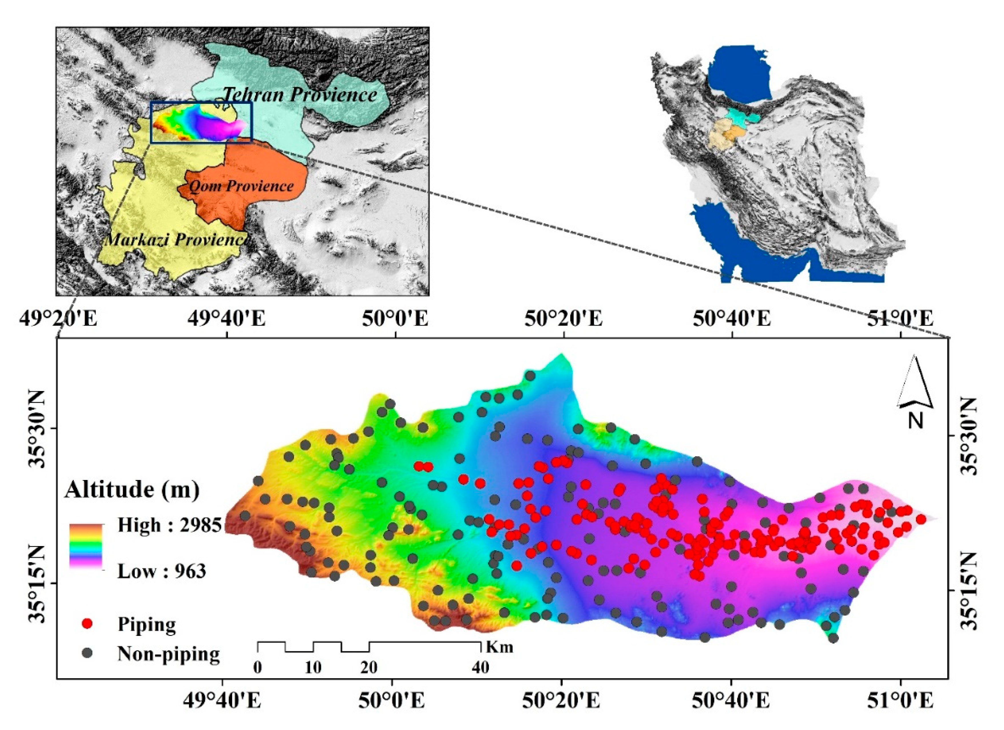
2.1. Description of the Study Area
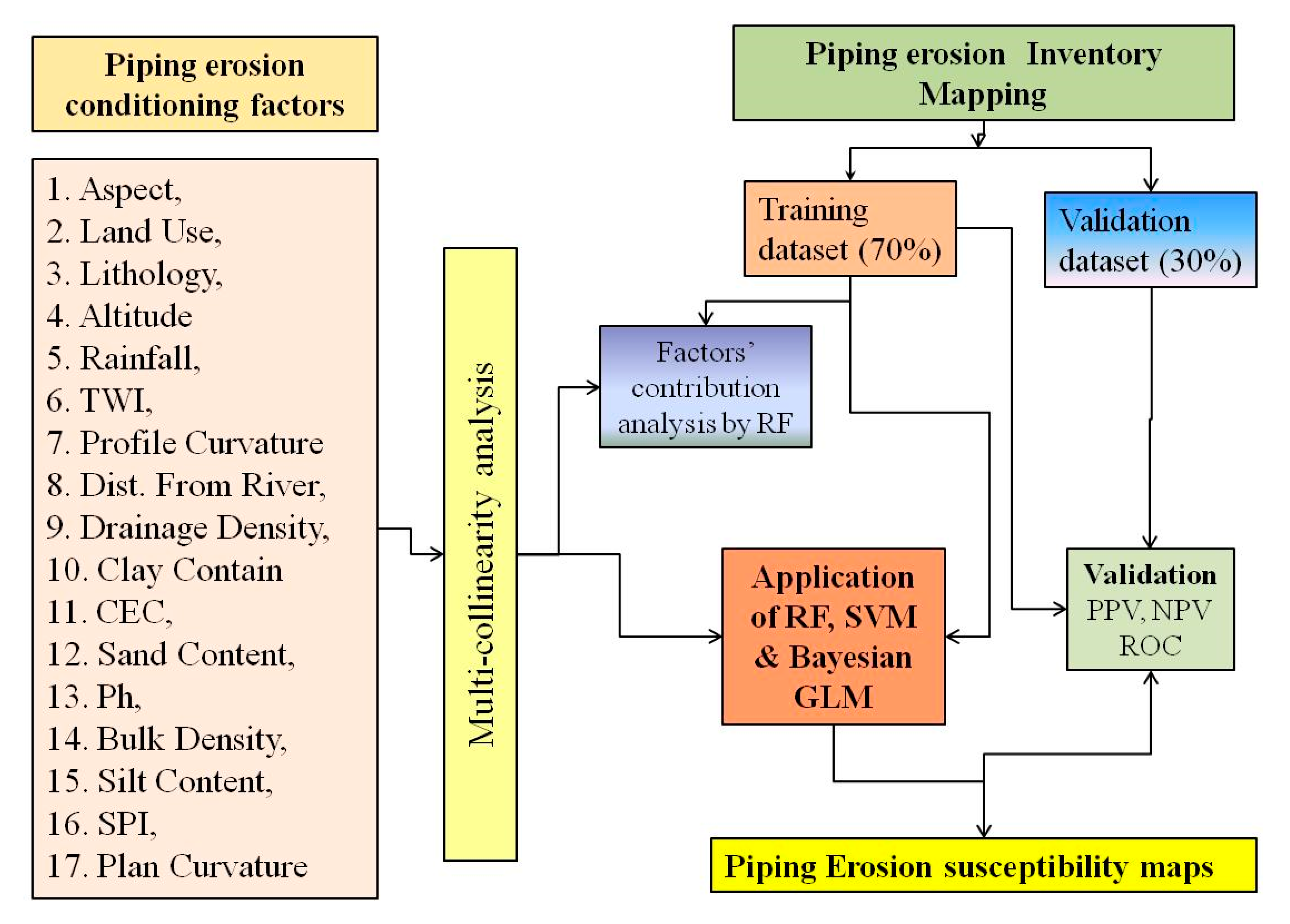
The Zarandieh watershed is located in the northern area of the Markazi province in Iran. This watershed is one of the sub-catchments of the Shoor river that is located at 35°10′ to 35°38′ N latitude and 49°40′ to 51°04′ E longitude, respectively (Figure 1). The catchment area is around 3592 km2, with an average elevation of 1974 m and an average slope of 3.2%. According to the climatic classification of the Zarandieh watershed, it is located in the arid and cold arid climates of the desert, with an average rainfall of 343 mm, with the highest rainfall occurring in winter. Land uses in the area include agricultural, bare land, rangeland, and residential land; most of the study area is rangeland. Most of the piping affected land is located in the eastern and center regions of the watershed, which are mainly agricultural and bare land. The soil of the Zarandieh watershed is deep, saline, and alkaline and, at the surface, saline. The most important limitations in this area are soil texture, salinity, alkalinity, and lack of drainage. The soils are generally deep and sometimes semi-shallow to calcareous and calcareous and articular (Administration of Natural Resources, Markazi Province https://markazi.frw.ir/00/Fa/default.aspx). The soils of the Zarandieh watershed are prone to erosion due to climatic conditions and the presence of highly saline soils, especially piping erosion due to the low slope of the region, and this erosion is one of the main problems in the region. Examples of piping erosion in the study area are shown in Figure 2.

2.2. Methods

The present study illustrates the usage of various machine learning methods in piping erosion susceptibility. Preparing the piping erosion susceptibility maps in the current research involved data collection, inventory map preparation, effective factors preparation, collinearity test, piping erosion susceptibility (PES) mapping using random forest (RF), support vector machine (SVM), and Bayesian generalized linear models (Bayesian GLM), factors importance analysis using the RF, and validation of the models (Figure 3). The piping erosion susceptibility maps were classified into five categories using the natural break method of Jenks [55].

2.3. Dataset Preparation for Spatial Modeling

Extensive field survey was carried out to determine the areas of piping erosion in the Zarandieh watershed in Markazi province. In this study, the location of each piping was determined using Garmin GPSMap (Garmin Ltd., Olathe, KS, USA) based on field vists. Moreover, a digital elevation model (DEM) with a spatial resolution of 12.5 m was downloaded from the Alaska Satellite Facility website (asf.alaska.edu) to investigate the location of the piping erosion susceptibility in the study area. Factors such as slope, aspect, distance from river, distance from road, topographic wetness index (TWI), topographic position index (TPI), rainfall, lithology, land use, drainage density, bulk density, pH, cation exchange capacity (CEC), silt, clay, and sand to map piping erosion susceptibility were used (Figure 3). Soil physical and chemical properties of the study area (pH, CEC, bulk density, sand, clay, and silt) were prepared from the SoilGrids site (https://soilgrids.org/) with a spatial accuracy of 250 m due to the large extent of the area and the lack of soil studies. Layers of topographic wetness index (TWI), topographic position index (TPI) were also prepared using SAGAGIS 3.2 software. Finally, 152 piping locations were recorded in the study area. In addition, 152 absence points were created using ArcGIS 10.5 software randomly (Figure 4). The piping points and the non-piping points were divided in two parts: 70% for training and 30% for validation.

2.4. Multi-Collinearity Analysis

Addressing the multicollinearity issue of the independent variables is quite necessary to understand their strength of predicting susceptibility and it can directly be depicted with the help of VIF [56]. VIF (variance inflation factor) is the second measure of multi-collinearity analysis, derived from the tolerance (reciprocal of VIF), which is the direct measure [56]. The consideration of VIF as less than 10 (for weaker models, it is less than 5) indicates no multi-collinearity problem and it is ready for further use in terms of prediction [36,50,56,57,58,59]. The equations of tolerance and VIF are as follows (Equations (1) and (2)):
Tolerance = 1 − R2J
VIF = 1/Tolerance
where R2J represents the regression coefficient of determination of explanatory variable J on all the other explanatory variables.

2.5. Machine Learning Method Used in Modeling the Piping Erosion

2.5.1. Random Forest (RF)

The random forest method is a relatively complex method among tree methods in which several decision trees are trained to increase model accuracy. The result is the prediction of a group of decision trees. In the random forest learning method, each decision tree is trained using a random sample selected from the training dataset [60]. Selecting a set of predictor variables used to segment the nodes is also done at random. In the random forest method, the mtry and ntree properties are determined for the covariates used in each subset and the number of trees used in the forest, respectively. The number of variables can range from one to the total number of covariates. The number of trees is selected by the user, usually from 500 to 1000 [60].
In the random forest algorithm, it is possible to select the most important and effective covariates. Estimation of the importance of a variable is done by queuing the values of each variable in the out-of-bag (OOB) samples, which are usually 1.3 observations, not used in the model, and by reclassifying the OOB samples using the row variable. OOB error change is used as a measure of variable importance. Variables whose deletion results in a relatively higher increase in OOB error are considered more important variables [43]. In the random forest method, each tree is formed as follows: (i) If N is the number of states in the training dataset, N state will randomly sample by pasting in the original data. This is an example of a work set for this tree; (ii) If there are M variables, consider m smaller than M such that at each node, m variables are randomly selected from M and the best separation of this m variable is used to separate the node. The value of m is assumed to be constant during forest construction, and (iii) each tree grows as large as possible. There is no pruning.

2.5.2. Support Vector Machine (SVM)

The structure of the support vector machine model was introduced by Vapnik [61] and it utilizes the principle of structural error minimization. The support vector machine models are divided into two main groups: support vector machine classification model and support vector machine regression model. Support vector machine classification models are used to solve data classification problems that are placed into different classes, and support vector regression models are used to solve forecasting problems. If the data are linearly separated, the equation is as follows (Equation (3)):
y = f ( x ) = sign [ i = 1 n y i α i x i , x j + b ]
If the data are not linearly separable, the samples can be pre-processed by transferring the samples to a non-linear space with high dimensionality, where the result is internal multiplication and proves that if a symmetric kernel of equation conditions Mercer application to the low-dimensional input space can be seen as the result of high-dimensional internal multiplication and greatly reduces computation [62]. In this case, Equation (3) is changed to Equation (4):
y = f ( x ) = sign [ i = 1 n y i α i K ( x i , x j ) + b ]
The K ( x i , x j ) function is a kernel function that produces internal multiplication to create machines with different types of nonlinear decision-making levels in the data space. Different kernels are used for the support vector machine regression model (Table 1).

2.5.3. Bayesian Generalized Linear Models (Bayesian GLM)

Bayesian reasoning is a probability-based approach to inference. The basis of this approach is that there is a probability distribution for each quantity, which can be optimized by observing new data and arguing about its probability distribution [63,64]. Bayesian networks, also known as belief networks, belong to the family of probabilistic graphical models. These graphical structures are used to represent information in an uncertain field. Specifically, each node in the graph represents a random variable and the branches represent probabilistic dependencies between the variables. These conditional dependencies are often evaluated by specific statistical and probabilistic methods. Bayesian networks combine principles of graph theory, probability theory, computer science, and statistics. Bayesian networks provide efficient representation and computation of the probability distribution shared over a series of random variables. Besides this, Bayesian networks model the intensity of the relationship between variables quantitatively, allowing the conditional belief about them to be automatically updated by accessing new information [64,65].
The basis of Bayesian learning is Bayesian theory. This theory allows the calculation of the secondary probability based on the first probabilities:
P ( h | D ) = P ( D | h ) P ( h ) P ( D )
where P ( h | D ) is a posterior probability, P ( D | h ) is a likelihood, P ( h ) is prior probability, and P ( D ) is evidence. As can be seen, by increasing P(D), the value of P(h|D) decreases, because the higher probability of D being observed independently of h means that D has less evidence to support h.

2.6. Methods of Validation and Accuracy Assessment

In the present study, four statistical measures including sensitivity (TPR), specificity (TNR), precision (PPV), and negative predictive value (NPV) were used for evaluating the fitness of the used machine learning models. The positive and negative predictive values (PPV and NPV, respectively) are the proportions of positive and negative results in statistics and diagnostic tests that are true positive and true negative results, respectively. Greater values of these statistical tests indicate the better result of the models [43,66]. The model output was speculated by area under the curve (AUC) of receiver operating characteristic (ROC) [67].
TPR = TP ( TP + FN )
TNR = TN ( TN + FP )
PPV = Number of positives ( Number of positives + Number of false positives )
NPV = Number of true negatives ( Number of true negatives + Number of false negatives )
AUC = TP + TN P + N
Finally, for all modeling approaches and analyses, we used R 3.5.2 software. The randomForest, e1071, arm packages were used to run the RF, SVM, and Bayesian GLM models. The susceptibility values generated from RF, SVM, and Bayesian GLM models were taken to the GIS environment to prepare the PES maps.

3. Results

3.1. Multi-Collinearity Analysis

The variance inflation factor (VIF) values of the variables are shown in Table 2. The VIF values of all the variables are less than 5, indicating their independence and readiness for use in the models. Among the seventeen variables, clay has the highest VIF (3.93) and aspect has the lowest (1.13).

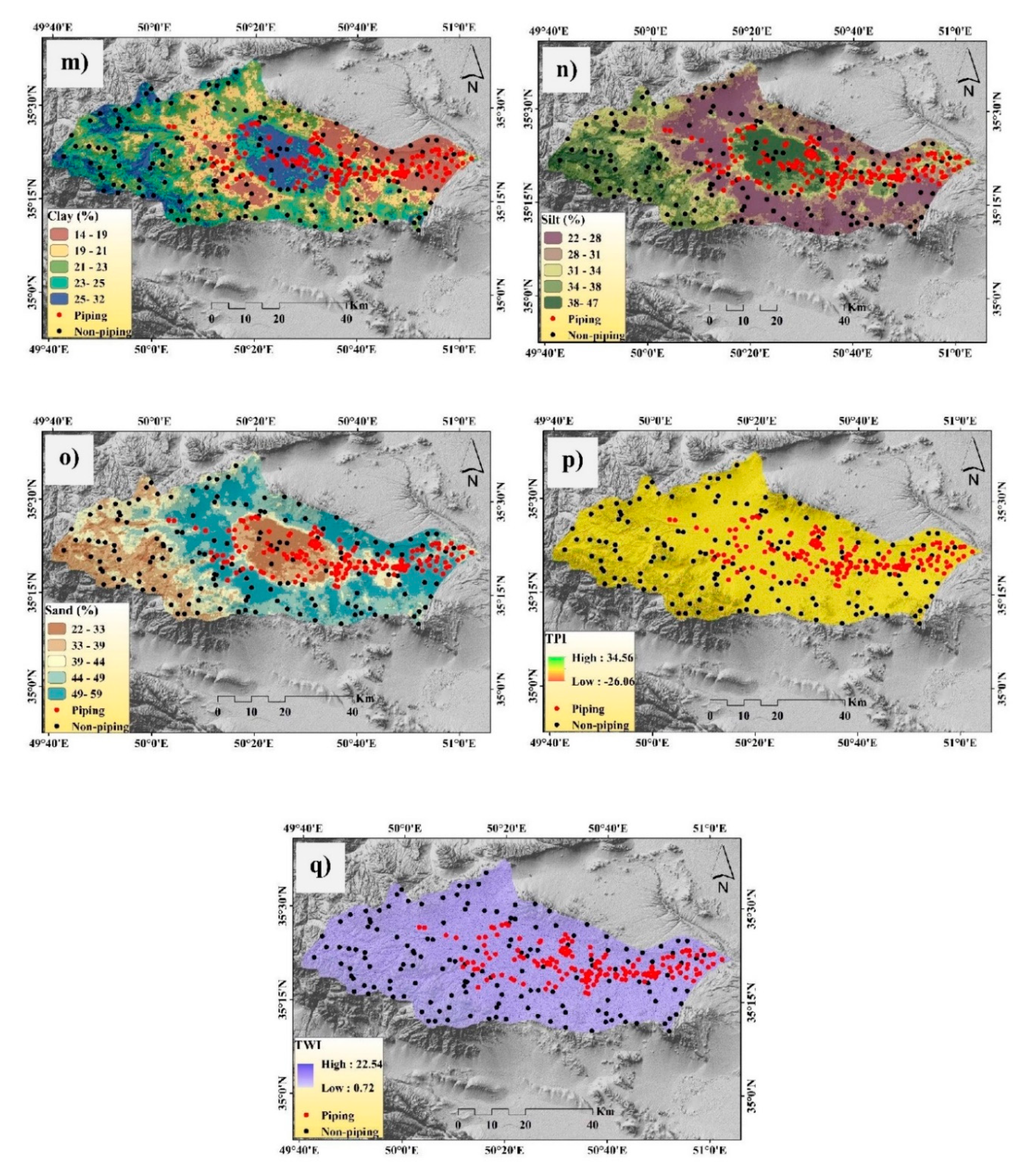
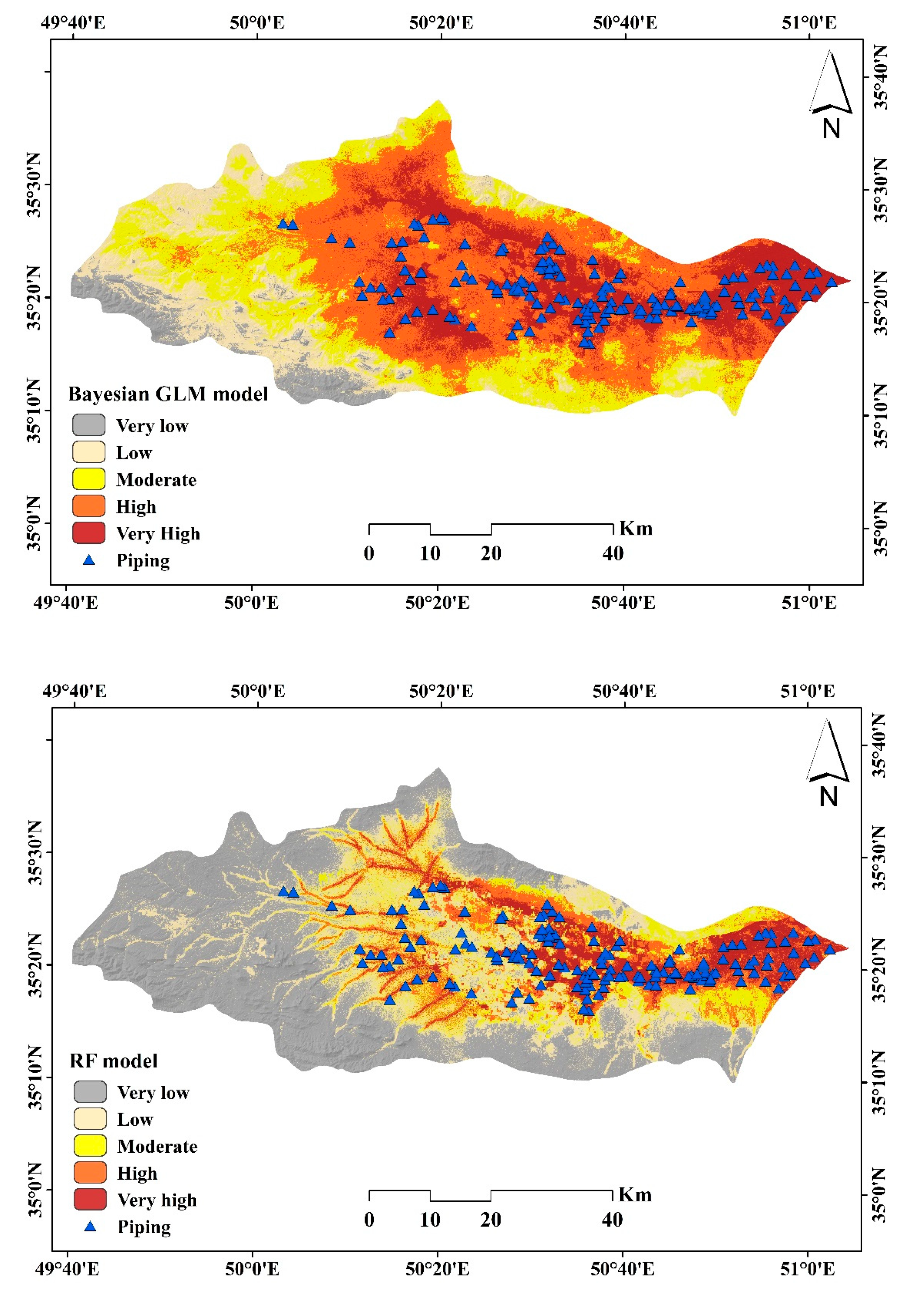
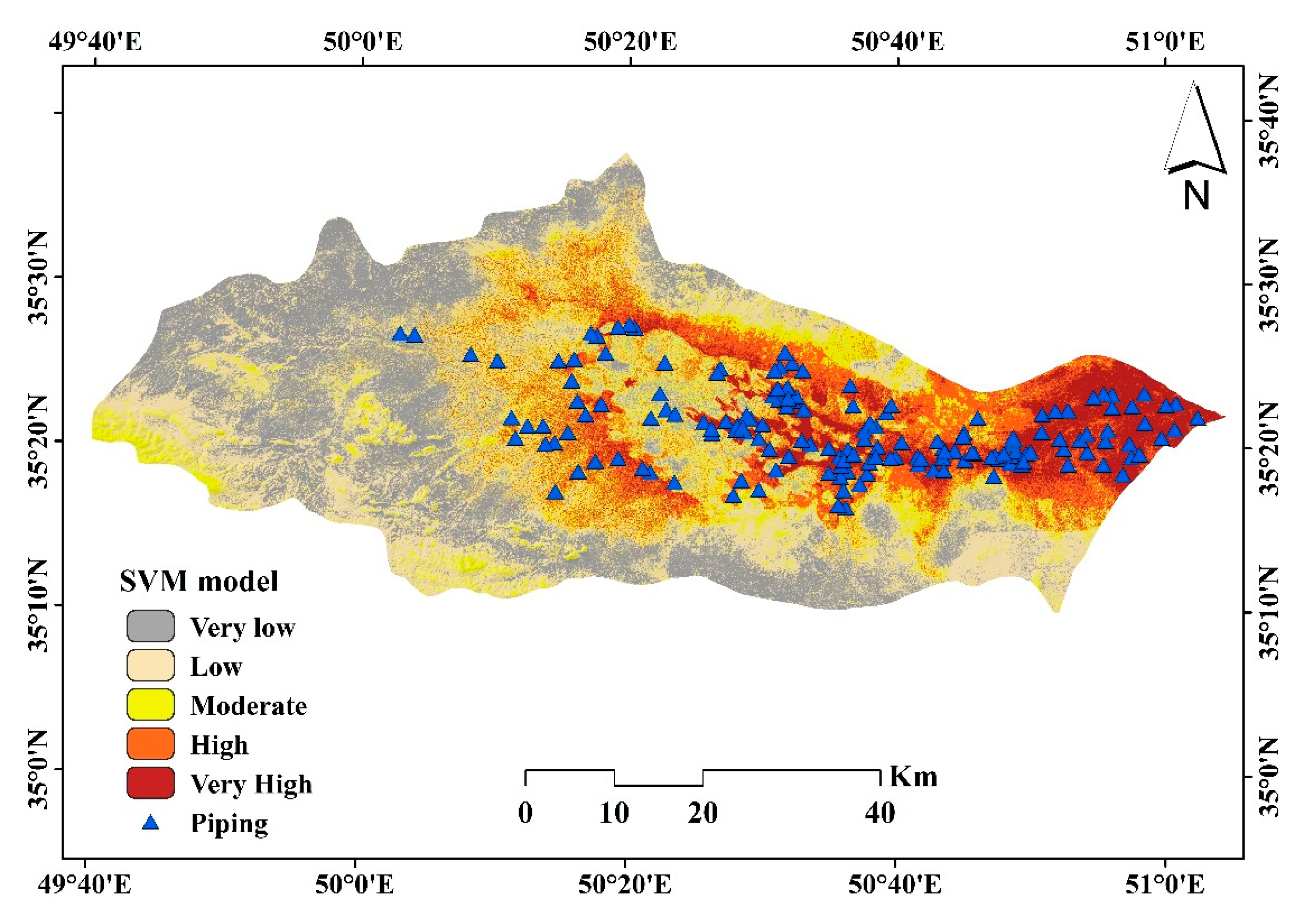
3.2. Piping Erosion Susceptibility Modeling

The piping and non-piping points containing the values of piping erosion susceptibility factors (PESFs) are taken as the input datasets in R 3.5.2 software to construct the piping erosion susceptibility (PES) models. Then, the PES maps are classified into five ordinal categories, i.e., very low, low, moderate, high, and very high based on the natural break classification method (Figure 5). The PES map generated from the RF model shows that very high and high PES zones account for 11.21% and 11.93% of the watershed area, respectively, whereas moderate, low, and very low PES zones cover 14.97%, 18.95%, and 42.93% of the area, respectively (Table 3). The SVM model also shows quite a similar picture to RF as very high and high PES zones occupy 11.5% and 14.59% of the basin area whereas moderate, low, and very low PES zones cover 19.33%, 29.4%, and 25.18% of the area, respectively. The very low PES zone according to the SVM model is significantly lower than the result of the RF model. However, as per the Bayesian GLM output, the very high and high PES zones account for 22.58% and 33.32% of the area, respectively, which is more than half of the basin area. This model shows the decreasing percentage of areas with piping erosion probability classes like moderate, low, and very low PES zones, which cover 24.41%, 14.22%, and 5.48% of the area, respectively. All three models identified that the downstream eastern end of the watershed is very highly susceptible to piping erosion. Among the models, Bayesian GLM shows more areas of high to very high PES zones (Figure 4). On the other hand, the southwestern end of the basin falls under very low PES zones, although the SVM model shows some share of moderate PES zones there. The map generated from the RF model shows a gully-like pattern in the PES zones of the central and western areas of the watershed.

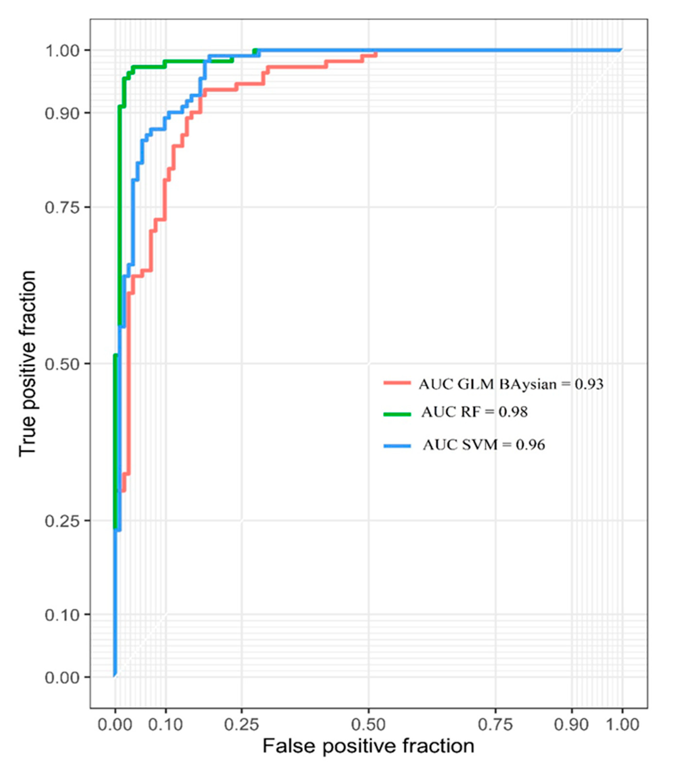
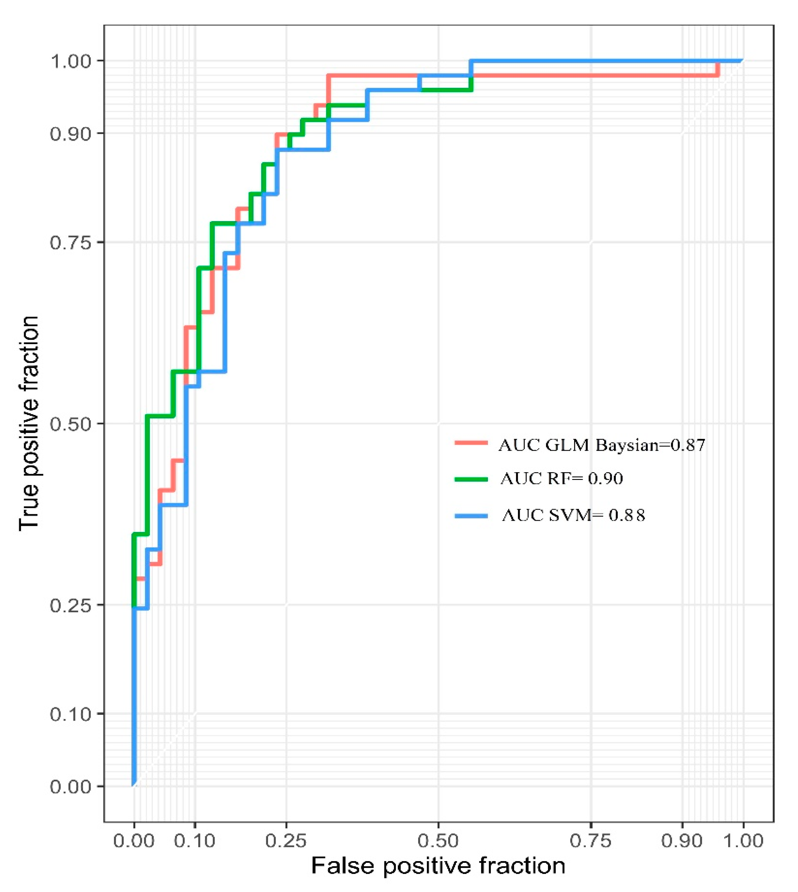
3.3. Validation of the Models

The piping erosion susceptibility (PES) maps by random forest (RF), SVM, and Bayesian GLM are justified by the receiver operating characteristics (ROC) curve using both the training and validation datasets (Figure 6 and Figure 7). As per the training datasets, the area under curve (AUC) values of RF, SVM, and Bayesian GLM are 0.98, 0.96, and 0.93, respectively (Table 4). The sensitivity (TPR) values of RF, SVM, and Bayesian GLM are 0.95, 0.891, and 0.80, respectively, which means that the areas detected as piping erosion susceptible zones by these models are very accurate. On the other hand, the specificity (TNR) values of RF, SVM, and Bayesian GLM models are 0.97, 0.893, and 0.89, respectively, which also indicates the high accuracy of the non-piping erosion susceptible zones detected by these models. The precision (PPV) values of these models are also high like RF (0.97), SVM (0.891), and Bayesian GLM (0.88), which shows the robustness of the models. Therefore, the parameters of validation for training datasets present excellent positive results in favor of these models.
Next, the validation datasets were used to examine the prediction capability of the three models. In the context of validation datasets, the AUC values of RF, SVM, and Bayesian GLM are 0.90, 0.88, and 0.87, respectively (Table 4). This suggests very good to excellent predictability of these three models. As per the ROC method, the sensitivity (TPR) values of RF, SVM, and Bayesian GLM are 0.89, 0.918, and 0.91, respectively, which means, as per the test datasets, these models also predicted correctly the piping erosion susceptible zones. The specificity (TNR) values of RF, SVM, and Bayesian GLM models are 0.74, 0.702, and 0.70, respectively, which suggests the decent prediction capability of the non-piping erosion susceptible zones also. The precision (PPV) values of these three models RF (0.78), SVM (0.762), and Bayesian GLM (0.76) indicate their decent ability of prediction. So, the results of the validation assessment suggest that the models used in the PES are very accurate and have high predictability.
Table 5 shows the importance of environmental factors in piping erosion modeling in the study area. Among these factors, altitude (9.29) has the highest importance for the piping susceptibility method, followed by pH, bulk density, and distance from the river (Table 5).

4. Discussion

4.1. Comparison of the Models

Piping erosion is a critical pedo-geomorphological process that contributes to land subsidence and gully formation in many parts of the world [68]. Piping erosion is more than a key topic in geomorphological research as it also affects agriculture production and triggers land degradation processes [12,15,69,70]. The subsurface dissolution of soil solutes can lead to the formation of underground channels, cavities which may trigger the sudden collapse of land or the creation of gullies and rills [71]. Therefore, the identification and proper prediction of the piping erosion susceptible zones in the watershed through mapping is crucial for a sustainable land management. Mapping can contribute to efforts to reduce the risk induced by sudden subsidence and collapses that can result in economic damages and casualties [72].
There are various methods and techniques which have been developed and executed all over the world for the prediction of piping erosion zones. The preparation of a rational and accurate susceptible map of piping erosion is a quite debatable matter for scientists. Recently, with the arrival of machine learning techniques, environmental modeling has become significantly accurate as these techniques can analyze the complex relationship between the predictors and responses like flood [73], gully erosion [74], landslide [75], and soil piping [76]. Many types of research are now being conducted to enhance the prediction performance of these models using various hybrid or ensemble algorithms. This work aims at applying machine learning models like RF, SVM, and Bayesian GLM for piping susceptible zoning of the watershed. Using sensitivity, specificity, PPV, NPV, and AUC values, the random forest (RF) model appeared as the best model in predicting the piping erosion susceptible zones. In the case of training datasets, the RF model performed best in all aspects. So, this model is best suited for the PES study and its success rate is excellent. However, in the case of sensitivity analysis of test datasets, the SVM model predicted the piping erosion zones more accurately than the other two.
The piping erosion can be addressed better with RF than SVM as per its design. RF generally uses the data as they are but SVM relies more on distance in a different linear or non-linear form, which might be the reason that RF is the best model here. Various non-linear kernels were used in SVM, which produced very good results in the end, and, in terms of predicting the future piping erosion zones, it was as the best model. Now, if we examine the results of Bayesian GLM, then we can see a similar picture to SVM. The validation values are nearly equal to SVM in all categories (Table 3) but the GLM model has produced more PES zones in high to very high categories than the other two. The sensitivity value of 0.80 and 0.91 in training and test datasets, respectively, suggests that the Bayesian GLM is also quite robust and suitable for PES assessment. One positive of using machine learning algorithms like RF, SVM, and Bayesian GLM is that they can automate the process of examining multiple databases to assemble the vital required information. These models can also identify the unique assumptions for decisions along with automatic large dataset analysis.

4.2. Variable Importance Analysis

The RF model, introduced by Breiman [77] by assimilating algorithms of decision tree [78,79], is useful for predicting and identifying independent variables’ contributions in the prediction process. Eighteen piping erosion susceptibility factors (aspect, altitude, plan curvature, profile, distance from the river, slope, TWI, lithology, land use, rainfall, TPI, silt, sand, clay, CEC, bulk density, and pH) were used in the modeling, evaluation of goodness-of-fit as well as performance of modeling processes. No variable showed a multi-collinearity problem, which indicates that all of them are independent factors and can be used in the modeling process. Among these factors, altitude (9.29) has the highest importance for the piping susceptibility method, followed by pH, bulk density, and distance from the river (Table 5). Lower elevation zones are more susceptible to piping erosion in comparison to the higher elevations, which is why we can see that very high PES zones exist in the lowest area of the watershed, in the eastern region. Bulk density has a positive relationship with the formation of pipes in the watershed, likely due to the formation of cracks on soils with high clay content, which are usually heavy soils. There is little known by other researchers about how bulk density behaves and impacts the origin and development of pipes [12,80] and our research shed light on this issue for the first time. Heavy textured soils can be seen now as a source of risk due to the development of piping via mainly the preferential flows developed. Researchers such as Jones [22] describe these as being responsible for quick catchment responses. Higher bulk density indicates higher compaction of the soil, which restricts the root growth to some extent, and this is also a factor to the development of bare land, gullies, rills, and badland areas, which is the landscape where piping is also very visible and abundant [23,81,82]. The influence of roots on piping development is relevant to understand whether plants contribute to piping development [83].
In the Zarandieh watershed, we found that the pH and CEC are also positive factors to develop pipes and this is because high rates of sodium are very common in piping areas. Other authors have shown that piping development is a physico-chemical process [84]. Our results demonstrate that the physico-chemical properties of the soil are more important to foresee the spatial distribution of piping erosion than the other parameters that were researched such as plan curvature, profile, aspect, or slope. The topographical characteristics of slopes and watersheds are not relevant to define the soil erosion losses and piping development as the soil chemical and physical properties are more relevant.
Another factor that was found relevant to foresee the risk of piping is the distance from the river. This is because the proximity to the river accelerates the process of piping erosion through the supply of sub-surface water. This process is well known in the formation of lakes and lagoons in semiarid land, where the formation of piping determines the drainage of the watersheds. A good example of this interaction between piping and groundwater is found in the paper of Castañeda et al. [85]. This has also been found as a source of risk, as was reported by Wang et al. [86], due to the formation of landslide dams as a consequence of piping erosion. Piping is a key landform to understand the rapid evolution of the landforms and our research confirms that few factors control the piping development. Masannat [87] already found in the Benson area in Arizona that overgrazing combined with the climatic conditions of long dry summers with intermittent short rain storms contributed to the initiation and development of piping erosion, and then piping triggered and developed gully erosion and badland morphologies. This is why Parker [88] already found that piping was a geomorphic agent in dry lands and that piping was a key actor in the semiarid landform development.
The study of piping erosion susceptibility in the study area shows that areas with agricultural land use are very sensitive to this type of erosion. Since the agricultural areas in the Zarandieh watershed have expanded to low slopes with soil which has a high salt content, agricultural operations in these areas have increased the infiltration of water and solute dissolution and led to the development of piping erosion. However, piping is a landform that, although widely present in arid and semiarid landscapes, is widespread around the world. It was found by Parker [89] on upland blanket peat, by Seppälä [90] and Carey and Woo [91] in the permafrost, and by Onda and Itakura [92] in rivers and temperate climatic conditions [93].

4.3. Implications and Soil Erosion Control

Our research demonstrates that it is possible to foresee where piping erosion will take place. However, to solve the problems caused by piping erosion, programs and strategies to reduce the soil losses should be developed. There is a need to control the high erosion rates found in piping areas around the world and strategies such as cover crops, mulches [94], catch crops [95], stone bonds [96], land abandonment [97], and reduced tillage should be applied on agricultural land to avoid the formation of soil erosion features such as pipes, rills, or gullies. It is on agricultural land that soil erosion problems are found around the world due to the abuse of the soil in vineyards and in persimmon, olive, citrus, and fruit tree plantations in semiarid land [9,98,99,100]. This is due to the low organic matter, which can solved with the use of organic farming strategies to restore the carbon content in the soil [101] and reduce the soil losses [102]. The above-mentioned strategies will contribute to improving the ecosystem services offered by the soil systems and to achieving sustainability challenges [94,103].

5. Conclusions

The Zarandieh watershed is very much susceptible to piping erosion and our research mapped the locations of it as well as the areas susceptible to land subsidence and gully erosion. Machine learning models (RF, SVM, and Bayesian GLM) have been used to assess the location of the piping areas. We considered 18 piping erosion conditioning factors from 304 locations. The models have shown that altitude, pH, bulk density, CEC, soil, and distance from the river are the key factors affecting piping erosion. We also noticed that the downstream area of the basin, along with fewer central areas, is highly to very highly susceptible to piping erosion. Therefore, from this study, it may be inferred that machine learning models can be used as a very accurate tool for managing piping erosion affected land.

Author Contributions

S.K.B. acquired the data; S.J., S.S.B., and A.M. conceptualized and performed the analysis; S.S.B., K.M., S.K.B., and M.S. wrote the manuscript, discussion, and analyzed the data; S.S. supervised and carried out funding acquisition; S.S.B. and A.C. provided technical insights, as well as edited, restructured, and professionally optimized the manuscript. All authors discussed the results and edited the manuscript. All authors have read and agreed to the published version of the manuscript.

Funding

This research received no external funding.

Acknowledgments

We acknowledge the support of the German Research Foundation (DFG) and the Bauhaus-Universität Weimar within the Open-Access Publishing Programme.

Conflicts of Interest

The authors declare no conflict of interest.

References

  1. Poesen, J.; Vandaele, K.; Van Wesemael, B. Gully erosion: Importance and model implications. In Modelling Soil Erosion by Water; Springer: Berlin/Heidelberg, Germany, 1998; pp. 285–311. [Google Scholar]
  2. Chaplot, V. Impact of terrain attributes, parent material and soil types on gully erosion. Geomorphology 2013, 186, 1–11. [Google Scholar] [CrossRef]
  3. Cerdà, A. Seasonal and spatial variations in infiltration rates in badland surfaces under Mediterranean climatic conditions. Water Resour. Res. 1999, 35, 319–328. [Google Scholar] [CrossRef]
  4. Cerdà, A.; Garcia-Fayos, P. The influence of slope angle on sediment, water and seed losses on badland landscapes. Geomorphology 1997, 18, 77–90. [Google Scholar] [CrossRef]
  5. Karamage, F.; Shao, H.; Chen, X.; Ndayisaba, F.; Nahayo, L.; Kayiranga, A.; Omifolaji, J.K.; Liu, T.; Zhang, C. Deforestation effects on soil erosion in the Lake Kivu Basin, DR Congo-Rwanda. Forests 2016, 7, 281. [Google Scholar] [CrossRef] [Green Version]
  6. Nicu, I.C. Is overgrazing really influencing soil erosion. Water 2018, 10, 1077. [Google Scholar] [CrossRef] [Green Version]
  7. Gomiero, T. Soil degradation, land scarcity and food security: Reviewing a complex challenge. Sustainability 2016, 8, 281. [Google Scholar] [CrossRef] [Green Version]
  8. Keesstra, S.D.; Bouma, J.; Wallinga, J.; Tittonell, P.; Smith, P.; Cerdà, A.; Montanarella, L.; Quinton, J.N.; Pachepsky, Y.; Van Der Putten, W.H.; et al. The significance of soils and soil science towards realization of the United Nations Sustainable Development Goals. Soil 2016, 2, 111–128. [Google Scholar] [CrossRef] [Green Version]
  9. Rodrigo-Comino, J.; Senciales González, J.M.; Cerdà Bolinches, A.; Brevik, E.C. The multidisciplinary origin of soil geography: A review. Earth-Science Reviews. Earth Sci. Rev. 2018, 177, 114–123. [Google Scholar] [CrossRef]
  10. Keesstra, S.; Mol, G.; De Leeuw, J.; Okx, J.; De Cleen, M.; Visser, S. Soil-related sustainable development goals: Four concepts to make land degradation neutrality and restoration work. Land 2018, 7, 133. [Google Scholar] [CrossRef] [Green Version]
  11. Poesen, J.; Nachtergaele, J.; Verstraeten, G.; Valentin, C. Gully erosion and environmental change: Importance and research needs. Catena 2003, 50, 91–133. [Google Scholar] [CrossRef]
  12. Diaz, A.R.; Sanleandro, P.M.; Soriano, A.S.; Serrato, F.B.; Faulkner, H. The causes of piping in a set of abandoned agricultural terraces in southeast Spain. Catena 2007, 69, 282–293. [Google Scholar] [CrossRef]
  13. Kariminejad, N.; Hosseinalizadeh, M.; Pourghasemi, H.R.; Bernatek-Jakiel, A.; Alinejad, M. GIS-based susceptibility assessment of the occurrence of gully headcuts and pipe collapses in a semi-arid environment: Golestan Province, NE Iran. Land Degrad. Dev. 2019, 30, 2211–2225. [Google Scholar] [CrossRef]
  14. Bernatek-Jakiel, A.; Poesen, J. Subsurface erosion by soil piping: Significance and research needs. Earth Sci. Rev. 2018, 185, 1107–1128. [Google Scholar] [CrossRef]
  15. Faulkner, H. Piping hazard on collapsible and dispersive soils in Europe. Soil Eros. Eur. 2006, 537–562. [Google Scholar]
  16. Bonelli, S.; Brivois, O.; Borghi, R.; Benahmed, N. On the modelling of piping erosion. Comptes Rendus Mécanique 2006, 334, 555–559. [Google Scholar] [CrossRef]
  17. Farifteh, J.; Soeters, R. Factors underlying piping in the Basilicata region, southern Italy. Geomorphology 1999, 26, 239–251. [Google Scholar] [CrossRef]
  18. Jones, J.A.A.; Richardson, J.M.; Jacob, H.J. Factors controlling the distribution of piping in Britain: A reconnaissance. Geomorphology 1997, 20, 289–306. [Google Scholar] [CrossRef]
  19. Verachtert, E.; Van Den Eeckhaut, M.; Poesen, J.; Deckers, J. Factors controlling the spatial distribution of soil piping erosion on loess-derived soils: A case study from central Belgium. Geomorphology 2010, 118, 339–348. [Google Scholar] [CrossRef] [Green Version]
  20. Deng, Q.C.; Zhang, B.; Luo, J.; Shu, C.Q.; Qin, F.C.; Luo, M.L.; Lin, Y.B. Types and controlling factors of piping landform in Yuanmou dry-hot valley. J. Arid Land Resour. Environ. 2014, 28, 138–144. [Google Scholar]
  21. Garcia-Ruiz, J.; Lasanta, T.; Alberto, F. Soil erosion by piping in irrigated fields. Geomorphology 1997, 20, 269–278. [Google Scholar] [CrossRef]
  22. Jones, J.A.A. Soil piping and catchment response. Hydrol. Process. 2010, 24, 1548–1566. [Google Scholar] [CrossRef]
  23. Gutierrez, M.; Sancho, C.; Benito, G.; Sirvent, J.; Desir, G. Quantitative study of piping processes in badland areas of the Ebro Basin, NE Spain. Geomorphology 1997, 20, 237–253. [Google Scholar] [CrossRef]
  24. Hosseinalizadeh, M.; Kariminejad, N.; Alinejad, M. An application of different summary statistics for modelling piping collapses and gully headcuts to evaluate their geomorphological interactions in Golestan Province, Iran. Catena 2018, 171, 613–621. [Google Scholar] [CrossRef]
  25. Mirhasani, M.; Rostami, N.; Bazgir, M.; Tavakoli, M. Threshold friction velocity and soil loss across different land uses in arid regions: Iran. Arab. J. Geosci. 2019, 12, 91. [Google Scholar] [CrossRef]
  26. Zare, M.; Mohammady, M.; Pradhan, B. Modeling the effect of land use and climate change scenarios on future soil loss rate in Kasilian watershed of northern Iran. Environ. Earth Sci. 2017, 76, 305. [Google Scholar] [CrossRef]
  27. Zare, M.; Panagopoulos, T.; Loures, L. Simulating the impacts of future land use change on soil erosion in the Kasilian watershed, Iran. Land Use Policy 2017, 67, 558–572. [Google Scholar] [CrossRef]
  28. Nosrati, K.; Collins, A.L. A soil quality index for evaluation of degradation under land use and soil erosion categories in a small mountainous catchment, Iran. J. Mt. Sci. 2019, 16, 2577–2590. [Google Scholar] [CrossRef]
  29. Vaezi, A.R.; Abbasi, M.; Bussi, G.; Keesstra, S. Modeling sediment yield in semi-arid pasture micro-catchments, NW Iran. Land Degrad. Dev. 2017, 28, 1274–1286. [Google Scholar] [CrossRef]
  30. Vaezi, A.R.; Hasanzadeh, H.; Cerdà, A. Developing an erodibility triangle for soil textures in semi-arid regions, NW Iran. Catena 2016, 142, 221–232. [Google Scholar] [CrossRef]
  31. Arabameri, A.; Cerda, A.; Rodrigo-Comino, J.; Pradhan, B.; Sohrabi, M.; Blaschke, T.; Tien Bui, D. Proposing a novel predictive technique for gully erosion susceptibility mapping in arid and semi-arid regions (Iran). Remote Sens. 2019, 11, 2577. [Google Scholar] [CrossRef] [Green Version]
  32. Parhizkar, M.; Shabanpour, M.; Khaledian, M.; Cerdà, A.; Rose, C.W.; Asadi, H.; Lucas-Borja, M.E.; Zema, D.A. Assessing and Modeling Soil Detachment Capacity by Overland Flow in Forest and Woodland of Northern Iran. Forests 2020, 11, 65. [Google Scholar] [CrossRef] [Green Version]
  33. Ostovari, Y.; Ghorbani-Dashtaki, S.; Bahrami, H.-A.; Naderi, M.; Dematte, J.A.M.; Kerry, R. Modification of the USLE K factor for soil erodibility assessment on calcareous soils in Iran. Geomorphology 2016, 273, 385–395. [Google Scholar] [CrossRef]
  34. Vandenboer, K.; Celette, F.; Bezuijen, A. The effect of sudden critical and supercritical hydraulic loads on backward erosion piping: Small-scale experiments. Acta Geotech. 2019, 14, 783–794. [Google Scholar] [CrossRef]
  35. Pereyra, M.A.; Fernández, D.S.; Marcial, E.R.; Puchulu, M.E. Agricultural land degradation by piping erosion in Chaco Plain, Northwestern Argentina. Catena 2020, 185, 104295. [Google Scholar] [CrossRef]
  36. Gayen, A.; Pourghasemi, H.R.; Saha, S.; Keesstra, S.; Bai, S. Gully erosion susceptibility assessment and management of hazard-prone areas in India using different machine learning algorithms. Sci. Total Environ. 2019, 668, 124–138. [Google Scholar] [CrossRef]
  37. Chen, W.; Chai, H.; Zhao, Z.; Wang, Q.; Hong, H. Landslide susceptibility mapping based on GIS and support vector machine models for the Qianyang County, China. Environ. Earth Sci. 2016, 75, 474. [Google Scholar] [CrossRef]
  38. Mustafa, M.R.U.; Sholagberu, A.T.; Yusof, K.W.; Hashim, A.M.; Khan, M.W.A.; Shahbaz, M. SVM-Based Geospatial Prediction of Soil Erosion Under Static and Dynamic Conditioning Factors. MATEC Web Conf. 2018, 203, 4004. [Google Scholar] [CrossRef]
  39. Pourghasemi, H.R.; Gayen, A.; Haque, S.M.; Bai, S. Gully Erosion Susceptibility Assessment Through the SVM Machine Learning Algorithm (SVM-MLA). In Gully Erosion Studies from India and Surrounding Regions; Springer: Berlin/Heidelberg, Germany, 2020; pp. 415–425. [Google Scholar]
  40. Amiri, M.; Pourghasemi, H.R.; Ghanbarian, G.A.; Afzali, S.F. Spatial Modeling of Gully Erosion Using Different Scenarios and Evidential Belief Function in Maharloo Watershed, Iran. In Advances in Remote Sensing and Geo Informatics Applications; Springer: Berlin/Heidelberg, Germany, 2019; pp. 253–256. [Google Scholar]
  41. Arabameri, A.; Rezaei, K.; Pourghasemi, H.R.; Lee, S.; Yamani, M. GIS-based gully erosion susceptibility mapping: A comparison among three data-driven models and AHP knowledge-based technique. Environ. Earth Sci. 2018, 77, 1–22. [Google Scholar] [CrossRef]
  42. Hosseinalizadeh, M.; Kariminejad, N.; Chen, W.; Pourghasemi, H.R.; Alinejad, M.; Mohammadian Behbahani, A.; Tiefenbacher, J.P. Spatial modelling of gully headcuts using UAV data and four best-first decision classifier ensembles (BFTree, Bag-BFTree, RS-BFTree, and RF-BFTree). Geomorphology 2019, 329, 184–193. [Google Scholar] [CrossRef]
  43. Avand, M.; Janizadeh, S.; Naghibi, S.A.; Pourghasemi, H.R.; Khosrobeigi Bozchaloei, S.; Blaschke, T. A Comparative Assessment of Random Forest and k-Nearest Neighbor Classifiers for Gully Erosion Susceptibility Mapping. Water 2019, 11, 2076. [Google Scholar] [CrossRef] [Green Version]
  44. Moradi, H.R.; Avand, M.T.; Janizadeh, S. Landslide susceptibility survey using modeling methods. In Spatial Modeling in GIS and R for Earth and Environmental Sciences; Elsevier: Amsterdam, The Netherlands, 2019; pp. 259–276. [Google Scholar]
  45. Arabameri, A.; Chen, W.; Loche, M.; Zhao, X.; Li, Y.; Lombardo, L.; Cerda, A.; Pradhan, B.; Bui, D.T. Comparison of machine learning models for gully erosion susceptibility mapping. Geosci. Front. 2019, 11, 1609–1620. [Google Scholar] [CrossRef]
  46. Amiri, M.; Pourghasemi, H.R.; Ghanbarian, G.A.; Afzali, S.F. Assessment of the importance of gully erosion effective factors using Boruta algorithm and its spatial modeling and mapping using three machine learning algorithms. Geoderma 2019, 340, 55–69. [Google Scholar] [CrossRef]
  47. Chen, W.; Yan, X.; Zhao, Z.; Hong, H.; Bui, D.T.; Pradhan, B. Spatial prediction of landslide susceptibility using data mining-based kernel logistic regression, naive Bayes and RBFNetwork models for the Long County area (China). Bull. Eng. Geol. Environ. 2019, 78, 247–266. [Google Scholar] [CrossRef]
  48. Javidan, N.; Kavian, A.; Pourghasemi, H.R.; Conoscenti, C.; Jafarian, Z. Gully Erosion Susceptibility Mapping Using Multivariate Adaptive Regression Splines—Replications and Sample Size Scenarios. Water 2019, 11, 2319. [Google Scholar] [CrossRef] [Green Version]
  49. Amiri, M.; Pourghasemi, H.R. Mapping and Preparing a Susceptibility Map of Gully Erosion Using the MARS Model. In Gully Erosion Studies from India and Surrounding Regions; Springer: Berlin/Heidelberg, Germany, 2020; pp. 405–413. [Google Scholar]
  50. Pourghasemi, H.R.; Yousefi, S.; Kornejady, A.; Cerdà, A. Performance assessment of individual and ensemble data-mining techniques for gully erosion modeling. Sci. Total Environ. 2017, 609, 764–775. [Google Scholar] [CrossRef] [Green Version]
  51. Gómez-Gutiérrez, Á.; Conoscenti, C.; Angileri, S.E.; Rotigliano, E.; Schnabel, S. Using topographical attributes to evaluate gully erosion proneness (susceptibility) in two mediterranean basins: Advantages and limitations. Nat. Hazards 2015, 79, 291–314. [Google Scholar] [CrossRef]
  52. Raja, N.B.; Çiçek, I.; Türkouglu, N.; Aydin, O.; Kawasaki, A. Landslide susceptibility mapping of the Sera River Basin using logistic regression model. Nat. Hazards 2017, 85, 1323–1346. [Google Scholar] [CrossRef] [Green Version]
  53. Arabameri, A.; Pradhan, B.; Pourghasemi, H.R.; Rezaei, K.; Kerle, N. Spatial modelling of gully erosion using GIS and R programing: A comparison among three data mining algorithms. Appl. Sci. 2018, 8, 1369. [Google Scholar] [CrossRef] [Green Version]
  54. Arabameri, A.; Cerda, A.; Tiefenbacher, J.P. Spatial pattern analysis and prediction of gully erosion using novel hybrid model of entropy-weight of evidence. Water 2019, 11, 1129. [Google Scholar] [CrossRef] [Green Version]
  55. Jenks, G.F. The data model concept in statistical mapping. Int. Yearb. Cartogr. 1967, 7, 186–190. [Google Scholar]
  56. Hair, J.F.; Black, W.C.; Babin, B.J.; Anderson, R.E.; Tatham, R.L. Multivariate Data Analysis; Prentice Hall: Upper Saddle River, NJ, USA, 1998. [Google Scholar]
  57. Saha, S. Groundwater potential mapping using analytical hierarchical process: A study on Md. Bazar Block of Birbhum District, West Bengal. Spat. Inf. Res. 2017, 25, 615–626. [Google Scholar]
  58. Roy, J.; Saha, S. GIS-based Gully Erosion Susceptibility Evaluation Using Frequency Ratio, Cosine Amplitude and Logistic Regression Ensembled with fuzzy logic in Hinglo River Basin, India. Remote Sens. Appl. Soc. Environ. 2019, 15, 100247. [Google Scholar]
  59. Roy, J.; Saha, S.; Arabameri, A.; Blaschke, T.; Bui, D.T. A Novel Ensemble Approach for Landslide Susceptibility Mapping (LSM) in Darjeeling and Kalimpong Districts, West Bengal, India. Remote Sens. 2019, 11, 2866. [Google Scholar]
  60. Breiman, L. Bagging predictors. Mach. Learn. 1996, 24, 123–140. [Google Scholar]
  61. Vapnik, V.N. The nature of statistical learning. In Theory; Elsevier: Amsterdam, The Netherlands, 1995. [Google Scholar]
  62. Burges, C.J.C. A tutorial on support vector machines for pattern recognition. Data Min. Knowl. Discov. 1998, 2, 121–167. [Google Scholar]
  63. Berry, D.A. Statistics: A Bayesian Perspective; Duxbury Press: Belmont, CA, USA, 1996. [Google Scholar]
  64. Bolstad, W.M.; Curran, J.M. Introduction to Bayesian Statistics; John Wiley & Sons: Hoboken, NJ, USA, 2016. [Google Scholar]
  65. Hoff, P.D. A First Course in Bayesian Statistical Methods; Springer: Berlin/Heidelberg, Germany, 2009. [Google Scholar]
  66. Ly, H.-B.; Monteiro, E.; Le, T.-T.; Le, V.M.; Dal, M.; Régnier, G.; Pham, B.T. Prediction and sensitivity analysis of bubble dissolution time in 3D selective laser sintering using ensemble decision trees. Materials 2019, 12, 1544. [Google Scholar]
  67. Arabameri, A.; Pradhan, B.; Rezaei, K.; Lee, C.-W. Assessment of Landslide Susceptibility Using Statistical- and Artificial Intelligence-Based FR–RF Integrated Model and Multiresolution DEMs. Remote Sens. 2019, 11, 999. [Google Scholar] [CrossRef] [Green Version]
  68. Boucher, S.C. Field Tunnel Erosion, Its Characteristics and Amelioration; Department of Conservation and Environment, Land Protection Division: Oklahoma City, OK, USA, 1990.
  69. Carey, S.K.; Woo, M.-K. The role of soil pipes as a slope runoff mechanism, Subarctic Yukon, Canada. J. Hydrol. 2000, 233, 206–222. [Google Scholar]
  70. Putty, M.R.Y.; Prasad, R. Runoff processes in headwater catchments—An experimental study in Western Ghats, South India. J. Hydrol. 2000, 235, 63–71. [Google Scholar]
  71. George, C.M.; Anu, V.V. Predicting piping erosion susceptibility by statistical and artificial intelligence approaches-A review. Int. Res. J. Eng. Technol. 2018, 5, 239–243. [Google Scholar]
  72. Liu, D.; Liang, X.; Chen, H.; Zhang, H.; Mao, N. A quantitative assessment of comprehensive ecological risk for a loess erosion gully: A case study of Dujiashi Gully, Northern Shaanxi province, China. Sustainability 2018, 10, 3239. [Google Scholar] [CrossRef] [Green Version]
  73. Chowdhuri, I.; Pal, S.C.; Chakrabortty, R. Flood susceptibility mapping by ensemble evidential belief function and binomial logistic regression model on river basin of eastern India. Adv. Space Res. 2020, 65, 1466–1489. [Google Scholar] [CrossRef]
  74. Gayen, A.; Pourghasemi, H.R. Spatial Modeling of Gully Erosion: A New Ensemble of CART and GLM Data-Mining Algorithms. In Spatial Modeling in GIS and R for Earth and Environmental Sciences; Elsevier: Amsterdam, The Netherlands, 2019; pp. 653–669. [Google Scholar]
  75. Youssef, A.M.; Pourghasemi, H.R. Landslide susceptibility mapping using machine learning algorithms and comparison of their performance at Abha Basin, Asir Region, Saudi Arabia. Geosci. Front. 2020, 79, 1–18. [Google Scholar] [CrossRef]
  76. Hosseinalizadeh, M.; Kariminejad, N.; Rahmati, O.; Keesstra, S.; Alinejad, M.; Behbahani, A.M. How can statistical and artificial intelligence approaches predict piping erosion susceptibility. Sci. Total Environ. 2019, 646, 1554–1566. [Google Scholar] [CrossRef]
  77. Breiman, L. Random forests. Mach. Learn. 2001, 45, 5–32. [Google Scholar] [CrossRef] [Green Version]
  78. Chen, X.-W.; Liu, M. Prediction of protein—Protein interactions using random decision forest framework. Bioinformatics 2005, 21, 4394–4400. [Google Scholar] [CrossRef]
  79. Zhang, K.; Wu, X.; Niu, R.; Yang, K.; Zhao, L. The assessment of landslide susceptibility mapping using random forest and decision tree methods in the Three Gorges Reservoir area, China. Environ. Earth Sci. 2017, 76, 405. [Google Scholar] [CrossRef]
  80. Holden, J. Controls of soil pipe frequency in upland blanket peat. J. Geophys. Res. Earth Surf. 2005, 110. [Google Scholar] [CrossRef] [Green Version]
  81. Torri, D.; Colica, A.; Rockwell, D. Preliminary study of the erosion mechanisms in a biancana badland (Tuscany, Italy). Catena 1994, 23, 281–294. [Google Scholar] [CrossRef]
  82. Piccarreta, M.; Faulkner, H.; Bentivenga, M.; Capolongo, D. The influence of physico-chemical material properties on erosion processes in the badlands of Basilicata, Southern Italy. Geomorphology 2006, 81, 235–251. [Google Scholar] [CrossRef]
  83. Bernatek-Jakiel, A.; Vannoppen, W.; Poesen, J. Assessment of grass root effects on soil piping in sandy soils using the pinhole test. Geomorphology 2017, 295, 563–571. [Google Scholar] [CrossRef]
  84. Romero-Diaz, A.; Ruiz-Sinoga, J.D.; Belmonte-Serrato, F. Physical-chemical and mineralogical properties of parent materials and their relationship with the morphology of badlands. Geomorphology 2020, 354, 107047. [Google Scholar] [CrossRef]
  85. Castañeda, C.; Gracia, F.J.; Rodriguez-Ochoa, R.; Zarroca, M.; Roqué, C.; Linares, R.; Desir, G. Origin and evolution of Sariñena Lake (central Ebro Basin): A piping-based model. Geomorphology 2017, 290, 164–183. [Google Scholar] [CrossRef] [Green Version]
  86. Wang, F.; Okeke, A.C.-U.; Kogure, T.; Sakai, T.; Hayashi, H. Assessing the internal structure of landslide dams subject to possible piping erosion by means of microtremor chain array and self-potential surveys. Eng. Geol. 2018, 234, 11–26. [Google Scholar] [CrossRef]
  87. Masannat, Y.M. Development of piping erosion conditions in the Benson area, Arizona, USA. Q. J. Eng. Geol. Hydrogeol. 1980, 13, 53–61. [Google Scholar] [CrossRef]
  88. Parker, G.G. Piping: A Geomorphic Agent in Landform Development of the Drylands; International Association of Scientific Hydrology: Wallingford, UK, 1964. [Google Scholar]
  89. Parker, A.P. Assessment and Extension of an Analytical Formulation for Prediction of Residual Stress in Autofrettaged Thick Cylinders. In Proceedings of the ASME 2005 Pressure Vessels and Piping Conference, Denver, CO, USA, 17–21 July 2005; pp. 67–71. [Google Scholar]
  90. Seppälä, M. Piping causing thermokarst in permafrost, Ungava Peninsula, Quebec, Canada. Geomorphology 1997, 20, 313–319. [Google Scholar] [CrossRef]
  91. Carey, S.K.; Woo, M. Hydrogeomorphic relations among soil pipes, flow pathways, and soil detachments within a permafrost hillslope. Phys. Geogr. 2002, 23, 95–114. [Google Scholar] [CrossRef]
  92. Onda, Y.; Itakura, N. An experimental study on the burrowing activity of river crabs on subsurface water movement and piping erosion. Geomorphology 1997, 20, 279–288. [Google Scholar] [CrossRef]
  93. Onda, Y. Seepage erosion and its implication to the formation of amphitheatre valley heads: A case study at Obara, Japan. Earth Surf. Process. Landf. 1994, 19, 627–640. [Google Scholar] [CrossRef]
  94. Sannigrahi, S.; Zhang, Q.; Joshi, P.K.; Sutton, P.C.; Keesstra, S.; Roy, P.S.; Pilla, F.; Basu, B.; Wang, Y.; Jha, S.; et al. Examining effects of climate change and land use dynamic on biophysical and economic values of ecosystem services of a natural reserve region. J. Clean. Prod. 2020, 257, 120424. [Google Scholar] [CrossRef]
  95. Cerdà, A.; Rodrigo-Comino, J.; Yakupouglu, T.; Dindarouglu, T.; Terol, E.; Mora-Navarro, G.; Arabameri, A.; Radziemska, M.; Novara, A.; Kavian, A.; et al. Tillage Versus No-Tillage. Soil Properties and Hydrology in an Organic Persimmon Farm in Eastern Iberian Peninsula. Water 2020, 12, 1539. [Google Scholar] [CrossRef]
  96. Guadie, M.; Molla, E.; Mekonnen, M.; Cerdà, A. Effects of Soil Bund and Stone-Faced Soil Bund on Soil Physicochemical Properties and Crop Yield Under Rain-Fed Conditions of Northwest Ethiopia. Land 2020, 9, 13. [Google Scholar] [CrossRef] [Green Version]
  97. Cerdà, A.; Ackermann, O.; Terol, E.; Rodrigo-Comino, J. Impact of farmland abandonment on water resources and soil conservation in citrus plantations in eastern Spain. Water 2019, 11, 824. [Google Scholar] [CrossRef] [Green Version]
  98. Novara, A.; Keesstra, S.; Cerdà, A.; Pereira, P.; Gristina, L. Understanding the role of soil erosion on CO2-C loss using 13C isotopic signatures in abandoned Mediterranean agricultural land. Sci. Total Environ. 2016, 550, 330–336. [Google Scholar] [CrossRef]
  99. Moradi, E.; Rodrigo-Comino, J.; Terol, E.; Mora-Navarro, G.; da Silva, A.N.; Daliakopoulos, I.; Khosravi, H.; Pulido Fernández, M.; Cerdà, A. Quantifying Soil Compaction in Persimmon Orchards Using ISUM (Improved Stock Unearthing Method) and Core Sampling Methods. Agriculture 2020, 10, 266. [Google Scholar] [CrossRef]
  100. Rodrigo-Comino, J.; Ponsoda-Carreres, M.; Salesa, D.; Terol, E.; Gyasi-Agyei, Y.; Cerdà, A. Soil erosion processes in subtropical plantations (Diospyros kaki) managed under flood irrigation in Eastern Spain. Singap. J. Trop. Geogr. 2020, 41, 120–135. [Google Scholar] [CrossRef]
  101. Novara, A.; Pulido, M.; Rodrigo-Comino, J.; Di Prima, S.; Smith, P.; Gristina, L.; Giminez-Morera, A.; Terol, E.; Salesa, D.; Keesstra, S. Long-term organic farming on a citrus plantation results in soil organic carbon recovery. Cuad. Investig. Geográfica 2019, 45, 271–286. [Google Scholar] [CrossRef] [Green Version]
  102. López-Vicente, M.; Calvo-Seas, E.; Álvarez, S.; Cerdà, A. Effectiveness of cover crops to reduce loss of soil organic matter in a rainfed vineyard. Land 2020, 9, 230. [Google Scholar] [CrossRef]
  103. Visser, S.; Keesstra, S.; Maas, G.; De Cleen, M. Soil as a basis to create enabling conditions for transitions towards sustainable land management as a key to achieve the SDGs by 2030. Sustainability 2019, 11, 6792. [Google Scholar] [CrossRef] [Green Version]
Figure 1. Location of Zarandieh Watershed in Iran.
Land 09 00346 g001
Figure 2. Pictures of piping erosion in Zarandieh watershed.
Land 09 00346 g002
Figure 3. Methodological flow chart: topographic position index (TWI), cation exchange capacity (CEC), stream power index (SPI), precision predictive value (PPV), negative predictive value (NPV), receiver operating characteristic (ROC)
Land 09 00346 g003
Figure 4. Piping erosion conditioning factors: (a) aspect, (b) land use, (c) lithology, (d) altitude, (e) rainfall, (f) TWI, (g) profile curvature, (h) distance from river, (i) drainage density, (j) clay content, (k) CEC, (l) sand content, (m) pH, (n) bulk density, (o) silt content, (p) SPI, (q) plan curvature.
Land 09 00346 g004aLand 09 00346 g004bLand 09 00346 g004c
Figure 5. Piping susceptibility map using the three models: Bayesian GLM, RF, SVM.
Land 09 00346 g005aLand 09 00346 g005b
Figure 6. The ROC curve analysis for three piping models using the training dataset.
Land 09 00346 g006
Figure 7. The ROC curve analysis for three piping models using the testing dataset.
Land 09 00346 g007
Table 1. Equations of different kernel functions.
ParametersEquationsKernel Function
- K ( x i , x j ) = x i · x j Linear kernel
γ and d K ( x i , x j ) = ( γ x i · x j + r ) d Polynomial kernel
γ K ( x i , x j ) = exp ( γ x i x j 2 ) Radial basis function kernel
Table 2. Multi-collinearity analysis to determine the linearity of the independent variables.
RowVariablesVIF
1Aspect1.13
2Altitude2.52
3Plan1.73
4Profile1.62
5Distance from river1.28
6Slope1.79
7TWI1.40
8Lithology1.49
9Land use1.41
10Rainfall3.62
11TPI1.51
12Silt2.58
13Sand1.89
14Clay3.93
15CEC1.88
16Bulk density2.96
17pH2.57
Table 3. Piping erosion susceptibility classes’ area.
Susceptibility ClassGLM BayesianSVMRF
Area (Km2)Area (%)Area (Km2)Area (%)Area (Km2)Area (%)
Very Low196.675.48904.5025.181542.1042.93
Low510.7414.221055.9829.40680.6618.95
Moderate876.7524.41694.2719.33537.8614.97
High1196.6533.32523.9814.59428.5611.93
Very High811.0422.58413.1111.50402.6411.21
Table 4. Predictive capability of piping models using train and test dataset.
ModelsSVMRFGLM Bayesian
Evaluation ParameterTestTrainTestTrainTestTrain
Sensitivity0.9180.8910.890.950.910.80
Specificity0.7020.8930.740.970.700.89
NPV0.8910.8930.870.950.890.82
PPV0.7620.8910.780.970.760.88
AUC0.880.960.900.980.870.93
Table 5. Variable importance analysis.
VariablesImportance
Aspect1.59
Altitude9.29
Plan curvature0.51
Profile curvature0.84
Distance from river4.47
Slope1.76
TWI2.76
Lithology0.78
Land use1.29
Rain0.18
TPI1.00
Silt1.46
Sand1.65
Clay0.90
CEC3.99
Bulk density6.81
pH8.80

