Impact of Land Use Changes on the Erosion Processes of a Degraded Rural Landscape: An Analysis Based on High-Resolution DEMs, Historical Images, and Soil Erosion Models

Abstract

Soil erosion is one of the major natural risk factors for developing high-value crops and an accurate estimation of spatial distribution and rates of soil degradation can be crucial to prevent crop degradation. In this paper, we use comparisons between high-resolution DEMs and soil erosion models to uncover the short-term landscape evolution of hazelnut crop yields, which are affected by incipient processes of rill development. Maps of rill initiation and evolution were extracted from the analysis of UAV-based multitemporal DEMs and the application of soil erosion models. A comparison between such a short-term analysis and historical orthophotos was carried out. Such a comparison shows how the USPED model predicts, very reliably, where linear erosion occurred. In fact, a reliable overlay between the linear erosive forms predicted by the USPED model and those captured by the UAV images can be observed. Furthermore, land use changes from 1974 to 2020 are characterized by a transition from abandoned areas (1974) to areas with high-value cultivation (2020), which has a strong impact on the spatial distribution of erosion processes and landslide occurrence. Such data represent a key tool for both the investigation of the spatial distribution of hot-spots of soil degradation and the identification of effective mitigation practices of soil conservation.

1. Introduction

Soil erosion is one of the most prominent natural risks in the rural landscapes of Mediterranean areas due to peculiar geological, geomorphological, and climate characteristics such as high relief, lithological features, and the rainfall regime [1]. The abandonment of rural areas has a strong influence on the spatial distribution of soil erosion processes since it can drive the relevant changes in several factors controlling geomorphological processes such as land cover, vegetation recovery, human-induced topographic modifications, and water runoff and infiltration [2]. Many works dealing with the impact of land abandonment have provided contrasting results, since the response to land abandonment in agricultural areas can increase or decrease the soil loss depending on several local factors such as climate setting, topographic features, the rainfall regime, and the type and magnitude of land cover changes/vegetation recovery [2,3,4]. In the arid and semi-arid landscapes of the Mediterranean region, a general trend of increase in soil loss can be observed [5,6,7]. Such an increase in soil loss has been frequently ascribed to natural and anthropic factors such as land abandonment and climate change [6,7]. An increase in the soil loss rate represents a critical issue for landscape management, the mitigation of geological risks, and land degradation. Soil loss rates are higher than the soil formation rates in the Mediterranean basin [8]. Mediterranean soils are easily eroded due to different characteristics: marked relief, 45% of the area having a slope greater than 8%; a high frequency of heavy rains in autumn and winter; poor, shallow, and skeletal soils; and sparse natural vegetation linked to severe summer droughts [9]. Several works have documented the strong impact of the abandonment of farming areas in the Mediterranean region on the hillslope degradation and the increase in the rates of erosion and landslide processes [10,11,12,13,14,15]. Land degradation and badland development is a common problem in the foredeep area of the southern Italian Apennine. This is as a consequence of human and natural factors such as climate setting, deforestation, widespread outcrops of silty clay, and high relief [10,16,17,18,19].

This work is part of a wider project named “Corylus, Sustainable hazelnut cultivation in Basilicata region” funded by the European Union as part of the program “Rural development 2014–2020”. The main objective of the project is to investigate the impact and sustainability of the intensive cultivation of hazelnuts on the rural landscapes of the Basilicata (Figure 1). The hazelnut crop was planted in 2018 and its possible impact on erosion processes has been verified through the visual inspection of historical images and UAV surveys.

The paths of the hazelnut tree in historical times were varied and do not allow a certain attribution of its origins. The movement of the hazelnut species from east to west, in the presence of a plant which has existed since prehistoric times, was widespread in classical times, as confirmed by the scientific term, which is composed of a Latinized Greek flanked by a Latin term (Corylus avellana). The coexistence of two names with different roots is a precise metaphor for the widespread diffusion of the hazelnut tree in the classical world, as evidenced by both historical sources [20,21] and recent studies [22]. Today, the hazelnut is a very ancient plant with a growing market demand and a high degree of adaption to pedological and morpho-climate conditions. Moreover, an analysis of historical sources highlights that hazelnut cultivation is widespread in southern Italy, mainly in landscape sectors affected by land abandonment and degradation. For these reasons, the local government authority and an international food company started an extensive project of planting hazelnut crops in different rural and degraded areas of southern Italy with the aim of: (i) increasing the social and economic growth of internal areas; (ii) promoting good practices of land management and mitigating the impact of land abandonment on the hillslope degradation of steep landscapes.

Extensive farming of internal areas with high-value cropland can be an effective solution to land abandonment and the related deterioration of the rural landscape [23] but these mitigation actions should be integrated by detailed monitoring and investigation of soil loss and land vulnerability estimations. Soil erosion models have been widely used as effective tools to assess the spatial distribution and the rates of erosion and deposition processes, but their calibration/validation is a critical issue [24,25]. The source to sink approach is one of the most used to evaluate the prediction ability of soil erosion models and it has been largely applied worldwide [25,26,27]. Alternative methods of evaluating the robustness of the prediction ability of soil erosion models can take advantage of the rapid increase in tools that are useful for the generation of multitemporal high-resolution DEMs, such as lidar surveys, UAV photogrammetry, and GPS surveys [28,29,30]. Among them, unmanned aerial vehicles (UAVs) have recently become an effective tool to obtain detailed information on the spatial and temporal distribution of different types of geomorphological processes such as gully erosion [31,32,33], fluvial dynamics [34], shoreline retreat [35], and mass wasting [36]. UAV-based photogrammetry, which generates digital elevation models (DEMs) from photo alignments, is a remarkable alternative to soil change measurements [33,37]. It offers many benefits, including a high data accuracy and the avoidance of any impact to the investigated surface. The use of UAV photogrammetry was made possible thanks to digital photogrammetry and computer vision that are part of the Structure from Motion (SfM) technique. Through the use of software based on SfM, it is possible to make 3D reconstructions of models starting from multiple images [38].

In this work, we estimated the spatial distribution of erosion and deposition through the application of the Unit Stream Power Erosion Deposition (USPED) model [39] in a catchment area in the eastern sector of the Basilicata region, southern Italy, (Figure 1), where a high-value crop has recently been planted. Validation of the model results has been carried out by comparing the USPED map with high-resolution DEMs deriving from the UAV workflow. After the preliminary evaluation of the robustness of the model results, we investigated the impact of the land use change (i.e., planting of hazelnut cropland) on the distribution and rates of the soil erosion processes.

2. Methods

The workflow of the study is summarized in Figure 2. After a detailed analysis of the geological, geomorphological, climate, and land use features of the study area based on classical and consolidated approaches such as field surveys, photo-interpretations, and DEM analysis, we prepared the basic parameter maps of the USPED model. More specifically, the following data were used to calculate the model parameters:

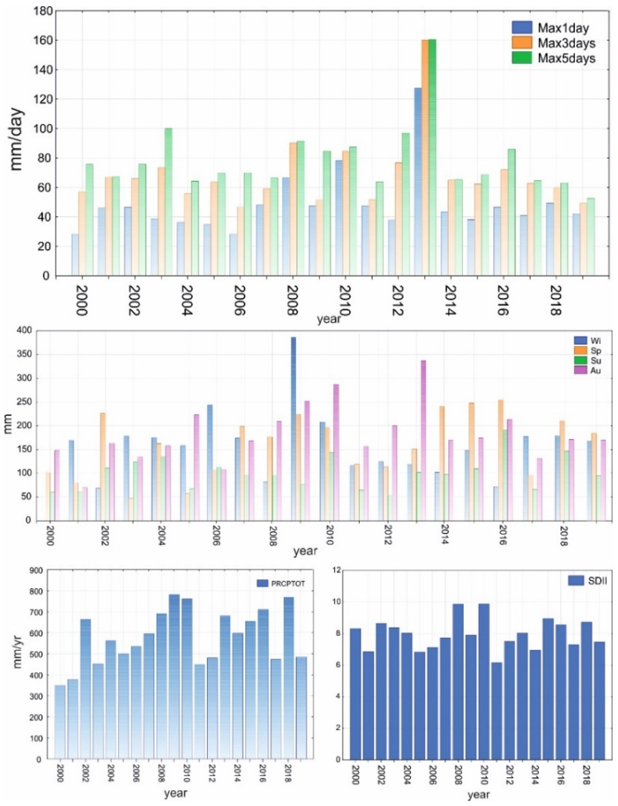
• Daily precipitation data, from the Irsina rain gauge (latitude 40.7486 and longitude 16.2394; period: 2000–2020);
• DEM with a spatial resolution of 1 m from an airborne LIDAR survey acquired in 2013;
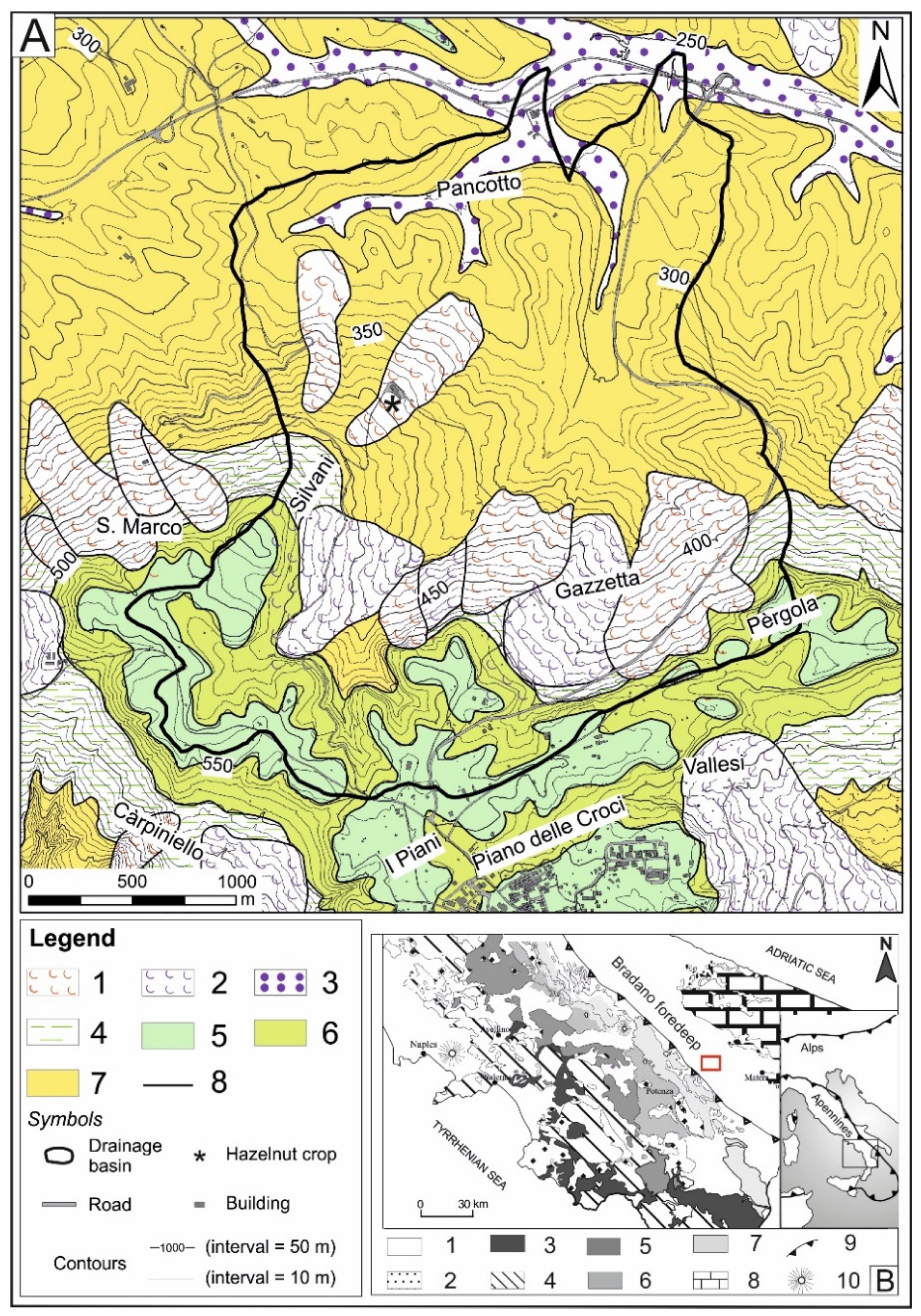
• Lithological map deriving from the official Italian geological map (Foglio 471 Irsina, [40]) and a detailed field survey;
• Land use map obtained from an inventory of land use/vegetation cover at a 1:5000 scale provided by the Basilicata Regional Authority (http://rsdi.regione.basilicata.it, accessed on 25 June 2021) and based on the procedures and recommendations of the Corine Land Cover project [41]. These data were combined with an interpretation of multi-years remote sensed images (Italian Geographic Military Institute, I.G.M.I. 1974 aerial photographs at a 1:15,000 scale; AGEA orthophotos at 1:10,000 scale, years: 2013 and 2017) to investigate historical land use changes over the last 40 years. These data were used to reconstruct the long-term land use changes and their impact on geomorphological processes (i.e., slope stability and erosion processes).

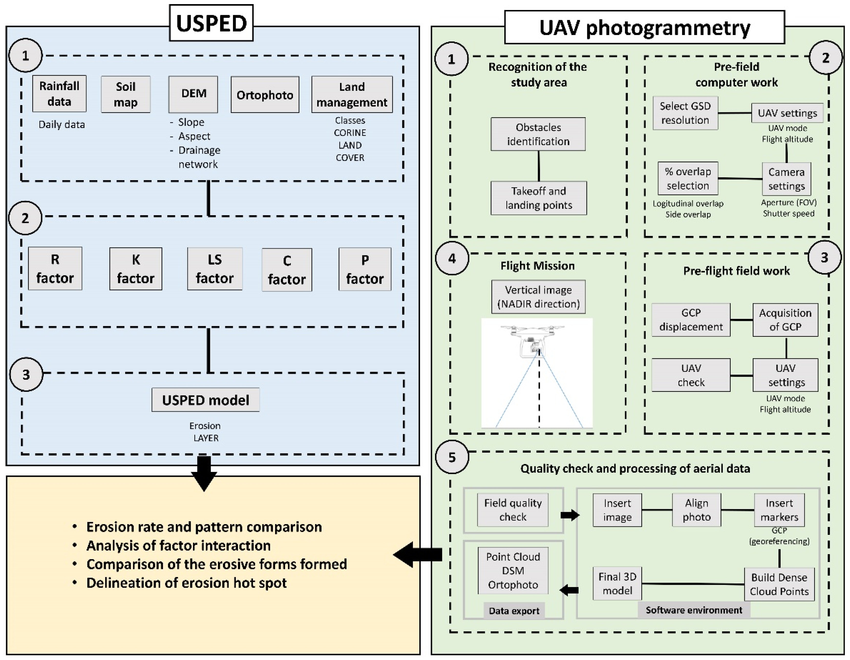
Finally, the results derived from the application of the USPED erosion model were compared with the photo-interpretations of the historical images and the short-term analysis of the erosion/deposition processes derived by the UAV-based high-resolution DEM. The UAV DEM was reconstructed as follows: DJI Phantom 3 Std UAV (Dà Jiāng Innovations, Shenzhen, China) was applied to take the photos, Leica Viva GS14 GNSS (Leica Geosystems, Heerbrugg, Switzerland) was applied to acquire the GCPs and a workstation was used for data processing.

2.1. USPED Model

The Unit Stream Power Erosion and Deposition (USPED) model estimates the average soil loss (A) using the basic structure of the RUSLE empirical equation [42]:

A = R × K × LS × C × P

where, A (Mg ha⁻¹ yr⁻¹) is the annual average soil loss, R (MJ mm h⁻¹ ha⁻¹ yr⁻¹) is the rainfall intensity factor, K (Mg h MJ⁻¹ mm⁻¹) is the soil erodibility factor, LS is the topographic factor, C (dimensionless) is the land cover factor and P (dimensionless) is the soil conservation or prevention practice factors [42].

The USPED model adopts an empirical equation for net erosion and deposition in a transport capacity limited regime, which differs from the RUSLE for the computation of the LS-factor. The equation, based on the upslope contributing area, has been developed by the authors of [39] to include topographic complexity by considering both the profile (in the downhill direction) and the tangential (perpendicular to the downhill direction) curvature [43,44]. Net erosion or deposition within a grid cell (ED) are computed as the divergence of sediment flow (change in sediment transport capacity) using the following equation [39,43]:

ED = ∂ [(A cos α)/∂ x] + ∂ [(A sin α)/∂ y]

where, α is the aspect of the terrain (in degrees). The physical basic assumption of the model is that net erosion pixels coincide with areas of profile convexity and tangential concavity (flow acceleration and convergence) while net deposition areas correspond to areas of profile concavity (decreasing flow velocity). The widespread use of semi-empirical erosion models such as RUSLE and USPED on a large scale is due to their relatively good degree of prediction ability with easily accessible data. As a matter of fact, many applications in different landscapes showing accurate results adopt simplified input parameters, which can be extracted by regional-scale and easily available data ([1,17,26,36,45], among others). A similar approach was used in this work, where detailed soil samples, small-scale plots of vegetation/soil features, and rainfall data at a high temporal resolution were not available. For these reasons, the spatial variations of the C- and K-factors were derived from land cover and lithological maps at a 1:5000 scale, whereas the R-factor was extracted from an empirical equation that correlated daily rainfall data with rainfall erosivity [46].

The R-factor depends on rainfall-runoff characteristics, which in turn are influenced by geographic location and altitude. In the original formulation of the USLE, the R-factor was calculated as the product of the total kinetic energy of the storm (E) and its maximum 30-min intensity (I30). Since this information was not available in the study area, we used the power-law equation proposed by the authors of [46] for the Basilicata region. This empirical equation was statistically derived from 20-min and hourly precipitation data higher than 10.0 mm. The formula is:

EI₃₀ = 0.1087 (P₂₄)^1.86

where, EI30 is the rainfall erosivity in MJ mm h⁻¹ ha⁻¹ yr⁻¹ and P₂₄ the daily rainfall amount in mm. The annual averaged R-factor value was estimated for the period from January 2010 to December 2020.

The soil erodibility factor (K) is the rate of soil loss per rainfall erosion index unit, Mg h MJ⁻¹ mm⁻¹, as estimated on a standard Wischmeier erosion plot [47]. The K-factor represents the soil profile response to the erosive power of rainfall events and was estimated using the following equation that includes soil texture and permeability:

K = 0.001317 [2.1 · 10⁻⁴ (12 − M) [(Si + fS)(100 − C)] 1.14 + 3.25(A − 2) + 2.5(P − 3)]

where, M is the organic matter content (%), Si is the silt fraction (%), 2 to 50 µm, fS is the fine sand content (%) 50 µ to 100 µm, C is the clay content (%) less than 2 µm, S is the sand content (%) 50 µm to 2 mm, A is the structure, and P is the permeability class (within the top 0.60–0.70 m) and the factor 0.001317 is derived from the division by 100 of the conversion value (0.1317) to the Si.

Texture, structure, and permeability data for each soil unit of the study area were extracted from previous works that have dealt with the physical and chemical characterization of deposits outcropping in the foredeep area of the southern Apennine chain [17,48,49,50]. The K-factor map was drawn by combining lithological and land use maps with the above-mentioned literature data about the texture and permeability of the main lithological units of the study area.

The topographic parameters, slope, and specific catchment area were derived from a 1 m DEM, deriving from a LIDAR survey acquired in 2013.

The modified LS-factor is given by the following relation:

LS [dimensionless] = (m + 1) (Ac/α0)^m (sin β0/0.0896)ⁿ

where, Ac (m) is the upslope contributing area per unit of width; β is the slope angle in degree; α0 is the length (72.6 ft, equal to 22.13 m) and β0 is the angle of the standard terrain (9%, equal to a 5.16 slope degree) of USLE/RUSLE. Finally, m (0.6) and n (1) are empirical exponents depending on the specific prevailing type of flow [39,43].

The C-factor (dimensionless), which reflects the effects of cropping and management practices on soil erosion rates, was calculated according to the literature data [51,52], with values assigned on the basis of the vegetative cover, its density, and the monthly rainfall runoff erosivity.

The information on land use was extracted from a detailed (i.e., 1:5000 scale) inventory of land use/vegetation cover provided by the Regional Spatial Data Infrastructure of the Basilicata Regional Authority (http://rsdi.regione.basilicata.it, accessed on 25 June 2021). The classification follows the procedures and recommendations of the Corine Land Cover project [41]. The C-values were assigned to the resulting 7 land use classes according to a revision of the C-values proposed in the literature (see for example [53]).

2.2. Photogrammetric Data of UAV-Based DEMs

In this work, the UAV DJI Phantom 3 Standard (quadricopter) was used to acquire the photos (

Table 1. Features of the Phantom 3 Standard and its camera.

#	Tool (A)	Parametres (B)	Value (C)
1		Flight time (min)	20–25
2		Weight (Battery & Propellers Included) (g)	1216
3	Phantom 3 std	Max distance (m)	1000
4		Max flight height (m)	500
5		Max wind resistence (m/s)	5.5–7.9
6		Focal lenght (mm)	35
7		ISO	100–1600
8	Camera	Sensor size	28.07 mm2 (6.17 mm × 4.56 mm)
9	Phantom 3 std	Sensor (px)	12 (4000 × 3000)
10		Aperture	f/2.8
11		Shutter speed	8–1/8000 s

). The drone was equipped with a stabilized camera, with a sensor able to compensate for involuntary movements due to the wind. In this way, the acquired images were guaranteed to have the correct orientation with respect to the ground. To ensure a high image resolution, the drone flew at a low elevation above the ground level (about 50 m). The drone recorded the coordinates for each photo through an internal GPS.

The features of the camera (Table 1) represent the essential factors for a good flight plan in addition to the resolution and the size of the sensor, especially the camera viewing angle (FOV–Field of View). In the flight plan, we selected the FOV value, the flight altitude, and the overlap percentage between adjacent swipes (side overlap). We calculated the shutter speed value to have a good percentage of longitudinal overlap (frontal overlap). We set a 60% side overlap and a frontal overlap of 80%. With these characteristics, the study area was covered with about 1100 photos. Agisoft Metashape (Agisoft LLC., St. Peterburg, Russia) was used to generate 3D models after the acquisition of the images (“Software environment” in Step 5 UAV Photogrammetry—Figure 2). The SfM algorithm calculated the position of the photos and the geometry of the scene, comparing all the images and finding the common points [54]. This process involved different steps. In the first step, homologous image points (Tie points) between the images were matched. In this way, the images were oriented in the space and a cloud of low-density points, namely, the dense sparse cloud, was created. Starting from this sparse cloud, a dense point cloud was built in the next step. In the last step, the DEM and orthophoto of the study area were built starting from the dense point cloud. The orientation of the 3D model and the generation of the DEM with a spatial resolution of 3.5 cm were drawn using 13 ground control points (GCPs) acquired by a RTK GPS.

3. Geological and Climate Setting

The study area was a small catchment area located in the foredeep of the southern Italian Apennine (Figure 3).

This sector of the chain is a hilly landscape characterized by widespread outcrops of a thick (i.e., several tens of meters) succession of marine grey-blue silty clays Early Pleistocene in age [55,56]. These deposits crop out in the central and northern sectors of the study area and are unconformably covered by marine to transitional coarser-grained clastic wedges, Early-Middle Pleistocene in age. They are composed of sand and gravel deposits and record the progressive emersion of the foredeep basin in response to the regional uplift of the southern Apennine chain [55,56,57]. Coarse-grain deposits are located in the headwater sectors of the catchment (Figure 3).

From a climate viewpoint, the study area exhibits a typical Mediterranean climate.

Daily rainfall records from the Irsina station in the last two decades highlight a mean annual value of total rainfall of 578 mm, with a strong seasonal variability and a prevalent concentration of rainfall in autumn and spring (Figure 4).

In general, the seasonal distribution of rainfall is shaped by dry summers and cold winters, and rainfall peaks occur in autumn. In this season, we observed heavy rainfall events related to one-day or multi-days of severe precipitation. An analysis of the recent trends in rainfall data suggest a general decrease in the total annual rainfall and an increase in both dry periods and short-term extreme events (Figure 4).

4. Results

4.1. Geomorphological Analysis

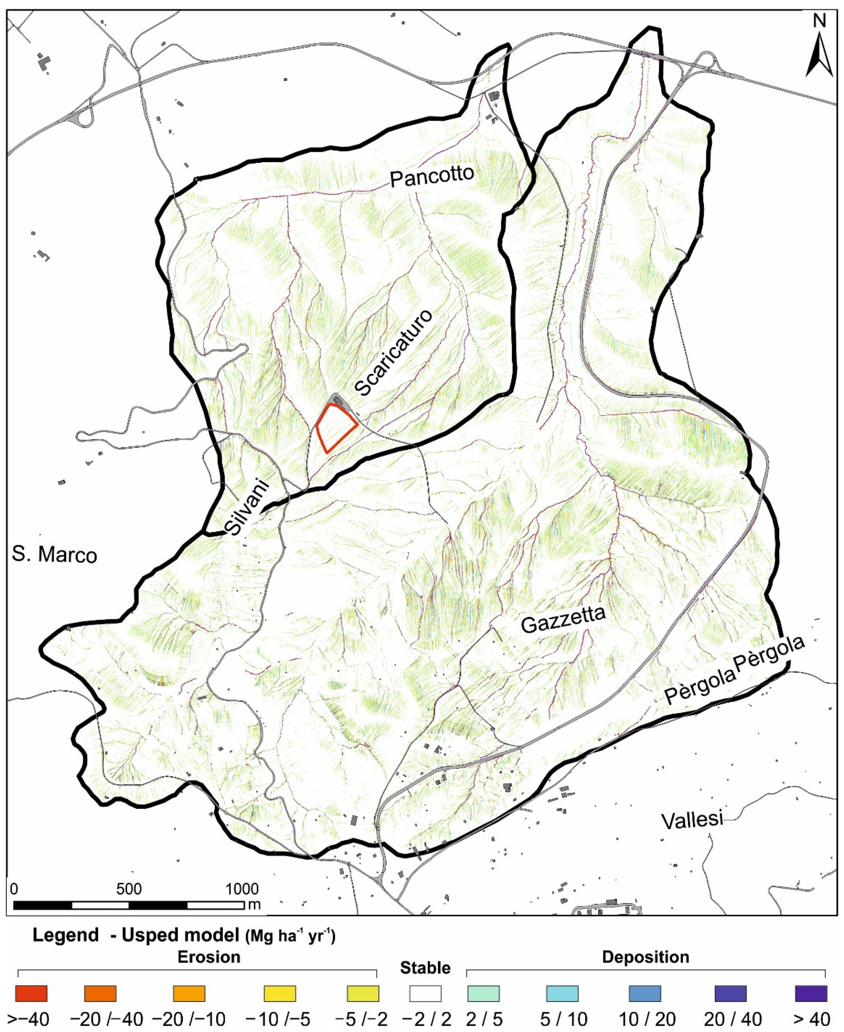
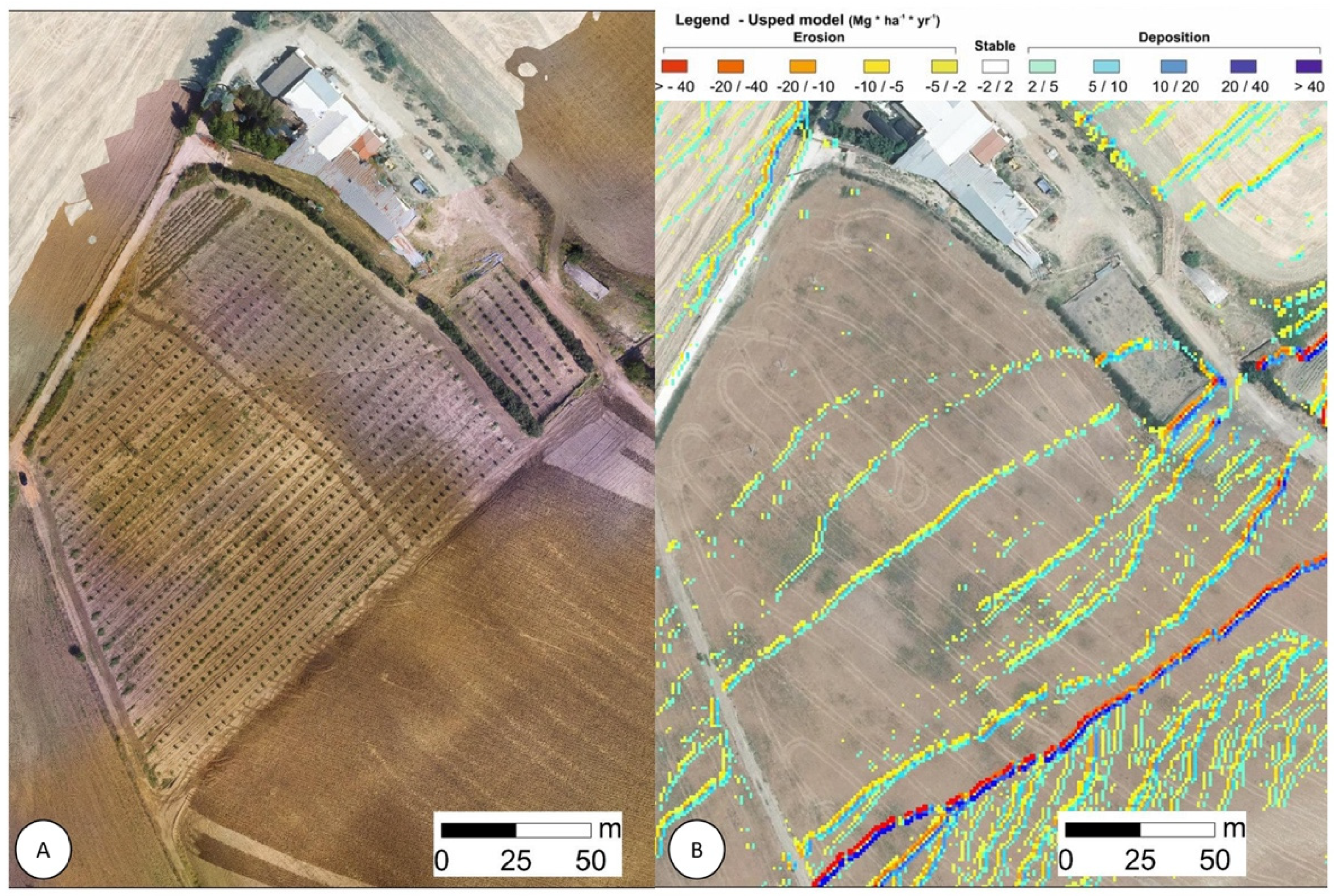
The study area included two catchment areas with elongated shapes, ranging in altitude from 500 to 210 m a.s.l. It covers a total area of about 7 kmq and is located along a SN-trending slope developing along the right-orographic side of the Basentello River. The studied catchment area is mainly carved in grey-blue silty clays and shows a north-dipping gentle slope (i.e., a mean slope of about 10°), which is transversally incised by a dendritic drainage network (Figure 1). Higher-altitude sectors of the study area are mainly carved in gravel deposits, thus exhibiting steeper slopes and higher relief. Channel incision, rills, and gullies developments are the main erosion processes of the study area, although small and shallow earthflows can be observed in the central and northern sectors of the catchment areas, where clay-rich lithological units crop out.

The present-day land use of the study area was derived from a digital inventory of the Basilicata Region (http://rsdi.regione.basilicata.it, accessed on 25 June 2021). It roughly follows the III level of the Corine Land Cover project [56] and highlights the prevalence of arable lands, which cover about 80% of the total catchment area. Natural grasslands and sclerophyllous vegetation represent the other relevant land use classes of the study area. They show a high level of degradation and are frequently affected by mass movement processes and accelerated linear erosion. Hazelnut cropland was also found in the catchment area.

4.2. USPED Model

The mean annual average erosivity factor computed for the study area using the hourly rainfall data of the Irsina rain gauge is equal to 664 MJ mm ha⁻¹ h⁻¹ yr⁻¹ for the 2000–2020 period.

The land use and land management factor (C-factor) in the drainage basin (Figure 5A) varies between a maximum value of 0.35 assigned to bare or degraded areas and a minimum value of 0.001 related to urban areas, roads, and small areas of broad-leaved forest. Intermediate values ranging from 0.1 to 0.25 were assigned to permanent crops (olive groves and hazelnut croplands), pastures, and arable lands. Lower values of the C-factor ranging from 0.025 to 0.035 were attributed to schlerophyllous vegetation and transitional woodland/sparse scrubs, respectively (Figure 5A).

The soil erodibility factor (K-factor) (Figure 5B) followed the stratigraphic contacts of the lithological map and ranged in the drainage basin between 0.02 Mg h MJ⁻¹ mm⁻¹ and 0.033 Mg h MJ⁻¹ mm⁻¹. The fine-grained clastic deposits outcropping in the intermediate and lower sectors of the catchments are inorganic silty clay, typically defined by a percentage of silt higher than 55–65% [50]. Coarser-deposits of the study area were composed of more sandy fractions and by a higher permeability, thus exhibiting higher values of the K-factor according to the Wischmeier equation. The assigned values of the K-factor are in accordance with similar estimations in adjacent areas of southern Italy (see for example [17]).

The terrain analysis showed a prevalence of areas with moderate slopes characterized by an average inclination lower than 12°. Accordingly, the average topographic LS-factor of the watershed (Figure 5C) is low, with an average of 1.74 and a standard deviation of σ = 22.6. Minimum LS-factor values occur in flat areas such as drainage divides.

The results of the application of the USPED model are shown in Figure 6. Each pixel has been classified using the following eleven classes of erosion/deposition:

1—Extreme erosion (>−40 Mg ha⁻¹ yr⁻¹)

2—High erosion (−20/−40 Mg ha⁻¹ yr⁻¹)

3—Moderate erosion (−10/−20 Mg ha⁻¹ yr⁻¹)

4—Low erosion (−5/−10 Mg ha⁻¹ yr⁻¹)

5—Very low erosion (−2/−5 Mg ha⁻¹ yr⁻¹)

6—Stable (−2/2 Mg ha⁻¹ yr⁻¹)

7—Very low deposition (2/5 Mg ha⁻¹ yr⁻¹)

8—Low deposition (5/10 Mg ha⁻¹ yr⁻¹)

9—Moderate deposition (10/20 Mg ha⁻¹ yr⁻¹)

10—High deposition (20/40 Mg ha⁻¹ yr⁻¹)

11—Extreme deposition (>40 Mg ha⁻¹ yr⁻¹)

The frequency distribution of the USPED model classes highlights that stable and low erosion/deposition areas of the study area cover about 84% of the entire catchment area, corresponding to a surface of about 6.1 kmq (Figure 7). The model results also indicate the diffuse presence of areas affected by extreme erosion and deposition, mainly located along the main channels of the drainage network. For example, the erosion surface area with values higher than 10 Mg ha⁻¹ yr⁻¹ is 0.23 kmq, which corresponds to about 3.1% of the whole catchment.

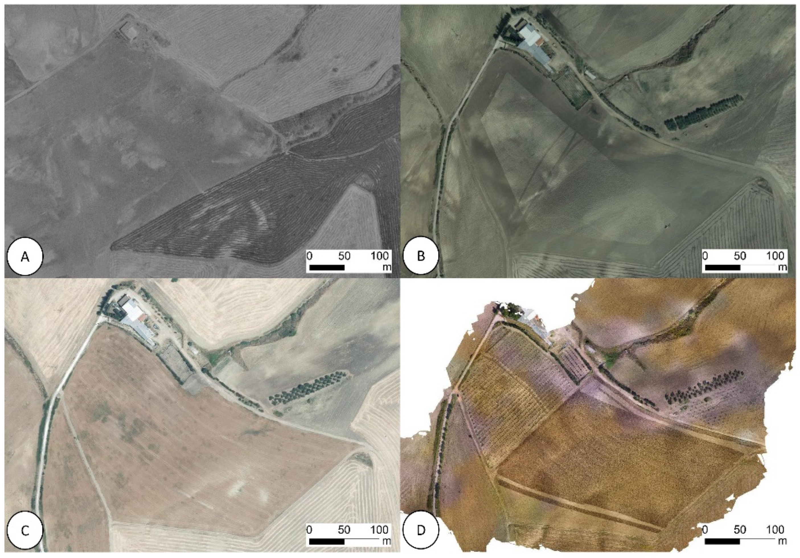
4.3. UAV Data and Landscape Changes

About 1060 photos were taken by UAVs at an altitude of 50 m. The results and timing of data processing, through the use of SfM, are summarized in

Table 2. Results of the workflow performed using Agisoft Metashape software.

	Value	Time
Photos	1062	-
Align photos (tie points)	4.4 × (105) points	1 h 17 min
Dense cloud Point	2.2 × (108) points	14 h 37 min
DEM	3.48 cm/px	10 min
Ortophoto	1.74 cm/px	29 min

.

The resolution of the DEM and of the orthophoto obtained (Table 2) underlines the high accuracy that can be obtained using this methodology. In fact, the errors of the 3D model on the Ground Control Points (GCP) resulted in: East 0.061 m; North 0.047 m; Altitude 0.092 m.

In the cultivated hazelnut area, linear erosive forms were observed (Figure 8A), which can be also observed in the USPED model map (Figure 8B).

The assessment of land use changes was completed using four different time periods: 1974, 2013, 2017, and 2020 (Figure 9).

Within the study area, two changes were observed in the investigated time period. In fact, when both changes are compared to 1974, it can be seen that the area occupied by the cultivation of hazelnuts in 2020 was abandoned in 1974. The abandonment is noticeable by the pronounced linear erosive forms and by the presence of small gravitational movements.

The other element that has undergone changes compared to 1974 is the position of the road to reach the hazelnut area (Figure 10).

Before 2017 (Figure 9), the study area was mainly used as arable land; the only change that can be seen compared to 2017 is the presence of hazelnut cultivation.

5. Discussion and Concluding Remarks

Many works have independently used soil erosion models and a multi-temporal analysis of aerial photos to investigate the spatial distribution and magnitude of geomorphological processes and the related control factors such as external forcing or anthropogenic impact [24,28,33,36,58,59,60,61,62,63]. Although land degradation and rural abandonment are frequently ascribed as relevant factors related to an increase in the occurrence and rates of linear and slope erosion processes [10,11,64,65], few studies have documented the role of cropland on the mitigation of geomorphological processes. In this work, we combined the USPED erosion model, a DEM derived from UAV photos, and an analysis of land use change from 1974 to 2020 to investigate the long- and short-term geomorphological processes of a rural landscape. These data were used to evaluate historical land use changes and their impact on the short- and long-term slope and fluvial processes of the study area. More specifically, we investigated the possible role of localized farming in the catchment area with high-value cropland as a sustainable action to prevent issues of land degradation and deterioration.

In foredeep areas of Basilicata, landscape remodeling activities and the use of machinery are typical agricultural practices in rural landscapes. Such practices are mainly related to cereal cultivation and several works have demonstrated their negative effect on soil erosion, landslide occurrence, badland development and, more generally, land degradation [17,23,50]. Land use changes from an abandoned area to widespread cultivation of cereals can then promote an increase in soil erosion and land degradation. On the contrary, the planting of more sustainable cropland such as hazelnut plants can represent a key strategy to prevent soil erosion and land degradation [23].

Our data are substantially based on a visual inspection of the multitemporal dataset and suggest a positive effect of farming practices (i.e., hazelnut cultivation) on the mitigation of slope processes and geomorphological processes. As a matter of fact, land use of the studied catchment area underwent several changes between 1974 and 2020. It was observed that in 1974 (Figure 9A), the central area was mostly disturbed by gravitational processes, which were not present in the images of the years 2013, 2017, and 2020 (Figure 9B–D). This difference is probably due to two factors that have changed over time: (i) change in land use; and (ii) change of the position of the road present in the western part of the images (Figure 10).

A short-term analysis of linear erosion processes based on the USPED model and its comparison with UAV images highlights that rill initiation and development is the main geomorphological process acting on the hazelnut cropland. In general, the comparison between the USPED erosion map and the DEM obtained from the SfM workflow demonstrates the reliability of the USPED in predicting the formation of linear erosion forms. Our results show that UAV images and the related data (i.e., ortophotos and high-resolution DEMs) can contribute to the identification of soil degradation with a similar ability to the soil erosion model. Such an integrated approach can represent a key-point in combining the validation and calibration of the two methods. The USPED model shows a diffuse and fairly superficial linear erosion (Figure 6). During the generation of the model parameters, the presence of the hazelnut area was inserted in the C-factor. As shown in Figure 8, the presence of the cultivated hazelnut favored the surface runoff following the rows of the hazelnut grove. The model predicted rills between the alignment of the hazelnut plant, which can be also observed by analyzing the UAV-based DEM. A relevant control factor for the spatial distribution of erosion processes is the position of the road (Figure 10): the modification of its location after the land use change from natural areas to agricultural land promoted the modification of the hydraulic conditions of this sector of the catchment area. In fact, linear elements such as trails and roads act as preferential routes along a slope for water flow [66]. In this way, the quantity of water received by the slope by runoff is reduced (Figure 10). The energy with which the water erodes is also reduced. This aspect is also highlighted by the USPED model (Figure 10D) and can be useful to drive the possible mitigation actions of erosion processes. Another important factor when calculating plantation erosion rates is the age of cultivation. In our case, the hazelnut plants were three years old, with an average height of 1.5 m and a poorly developed root system. The erosion rate of young plantations is higher than for older plantations, as demonstrated by Rodrigo Comino et al. (2017) [66] in vineyard plantations.

The study of land use dynamics and its impact on changes in soil properties and surface runoff will help toward the proper planning, management, and sustainable development of land resources [67]. The information can be employed to predict potential changes that would likely exist in the future. Furthermore, it can contribute information to allow good practices promoting soil conservation and mitigating land degradation to be undertaken. Our approach has a practical relevance since it can be useful for predicting localized areas of higher vulnerability or accelerated erosion.

In conclusion, the results show how the USPED erosion prediction model works well in areas characterized by steep slopes and poor soil cover. It also highlights how the cultivation of hazelnuts (high value), especially in the first years, can be affected by soil erosion and prevent the development of plants. This factor can have several negative effects, including slowing down the future harvest of hazelnuts with negative social and economic consequences. The cultivation of hazelnuts can also be an effective solution to land abandonment and the related deterioration of rural areas [23]. These mitigation actions should be integrated by detailed monitoring and an investigation of soil loss and land vulnerability estimations at a basin scale and can be applied to other areas with similar types of soil, climate, and socio-economic conditions.

References

1. Panagos, P.; Borrelli, P.; Poesen, J.; Ballabio, C.; Lugato, E.; Meusburger, K.; Montanarella, L.; Alewell, C. The new assessment of soil loss by water erosion in Europe. Environ. Sci. Policy 2015, 54, 438–447. [Google Scholar] [CrossRef]
2. Rodrigo-Comino, J.; Martínez-Hernández, C.; Iserloh, T.; Cerdà, A. Contrasted Impact of Land Abandonment on Soil Erosion in Mediterranean Agriculture Fields. Pedosphere 2018, 28, 617–631. [Google Scholar] [CrossRef] [Green Version]
3. Gusarov, A.V. The impact of contemporary changes in climate and land use/cover on tendencies in water flow, suspended sediment yield and erosion intensity in the northeastern part of the Don River basin, SW European Russia. Environ. Res. 2019, 175, 468–488. [Google Scholar] [CrossRef]
4. Özşahin, E.; Eroğlu, İ. Soil erosion risk assessment due to land use/cover changes (LUCC) in Bulgaria from 1990 to 2015. Alınteri Zirai Bilimler Dergisi 2019, 34, 1–8. [Google Scholar] [CrossRef]
5. Guo, Y.; Peng, C.; Zhu, Q.; Wang, M.; Wang, H.; Peng, S.; He, H. Modelling the impacts of climate and land use changes on soil water erosion: Model applications, limitations and future challenges. J. Environ. Manag. 2019, 250, 109403. [Google Scholar] [CrossRef]
6. Borrelli, P.; Robinson, D.A.; Fleischer, L.R.; Lugato, E.; Ballabio, C.; Alewell, C.; Meusburger, K.; Modugno, S.; Schütt, B.; Ferro, V.; et al. An assessment of the global impact of 21st century land use change on soil erosion. Nat. Commun. 2017, 8, 2013. [Google Scholar] [CrossRef] [PubMed] [Green Version]
7. Boardman, J.; Poesen, J.; Evans, R. Socio-economic factors in soil erosion and conservation. Environ. Sci. Policy 2003, 6, 1–6. [Google Scholar] [CrossRef]
8. Kosmas, C.; Danalatos, N.; Cammeraat, L.H.; Chabart, M.; Diamantopoulos, J.; Farand, R.; Gutierrez, L.; Jacob, A.; Marques, H.; Martinez-Fernandez, J.; et al. The effect of land use on runoff and soil erosion rates under Mediterranean conditions. Catena 1997, 29, 45–59. [Google Scholar] [CrossRef]
9. Raclot, D.; Le Bissonnais, Y.; Annabi, M.; Sabir, M. Challenges for mitigating Mediterranean soil erosion under global change. In The Mediterranean Region under Climate Change; IRD: Marseille, France, 2016; pp. 311–318. [Google Scholar]
10. Brandolini, P.; Pepe, G.; Capolongo, D.; Cappadonia, C.; Cevasco, A.; Conoscenti, C.; Marsico, A.; Vergari, F.; Del Monte, M. Hillslope degradation in representative Italian areas: Just soil erosion risk or opportunity for development? Land Degrad. Dev. 2018, 29, 3050–3068. [Google Scholar] [CrossRef]
11. Pepe, G.; Mandarino, A.; Raso, E.; Scarpellini, P.; Brandolini, P.; Cevasco, A. Investigation on farmland abandonment of terraced slopes using multitemporal data sources comparison and its implication on hydro-geomorphological processes. Water 2019, 11, 1552. [Google Scholar] [CrossRef] [Green Version]
12. Koulouri, M.; Giourga, C. Land abandonment and slope gradient as key factors of soil erosion in Mediterranean terraced lands. Catena 2007, 69, 274–281. [Google Scholar] [CrossRef]
13. Pardini, G.; Gispert, M. Impact of land abandonment on water erosion in soils of the Eastern Iberian Peninsula. Agrochimica 2006, 50, 13–24. [Google Scholar]
14. Lasanta, T.; García-Ruiz, J.M.; Perez-Rontome, C.; Sancho-Marcén, C. Runoff and sediment yield in a semi-arid environment: The effect of land management after farmland abandonment. Catena 2000, 38, 265–278. [Google Scholar] [CrossRef] [Green Version]
15. Lasanta, T.; Pérez-Rontomé, C.; García-Ruiz, J.; Machín, J.; Navas, A. Hydrological problems resulting from farmland abandonment in semi-arid environments: The central Ebro depression. Phys. Chem. Earth 1995, 20, 309–314. [Google Scholar] [CrossRef]
16. Clarke, M.L.; Rendell, H.M. Climate-driven decrease in erosion in extant Mediterranean badlands. Earth Surf. Process. Landf. 2010, 35, 1281–1288. [Google Scholar] [CrossRef]
17. Capolongo, D.; Pennetta, L.; Piccarreta, M.; Fallacara, G.; Boenzi, F. Spatial and temporal variations in soil erosion and deposition due to land-levelling in a semi-arid area of Basilicata (Southern Italy). Earth Surf. Process. Landf. 2008, 33, 364–379. [Google Scholar] [CrossRef]
18. Piccarreta, M.; Capolongo, D.; Boenzi, F.; Bentivenga, M. Implications of decadal changes in precipitation and land use policy to soil erosion in Basilicata, Italy. Catena 2006, 65, 138–151. [Google Scholar] [CrossRef]
19. Piccarreta, M.; Faulkner, H.; Bentivenga, M.; Capolongo, D. The influence of physico-chemical material properties on erosion processes in the badlands of Basilicata, Southern Italy. Geomorphology 2006, 81, 235–251. [Google Scholar] [CrossRef]
20. Regis, R. Il tipo corylus: Origini, riscontri, fortuna (con particolare riferimento al territorio italiano). Vox Roman 2009, 67, 11–33. [Google Scholar]
21. Bertoldi, V. Una voce moritura. Ricerche sulla vitalità di Corylus (>*Colurus). RLiR 1925, 1–2, 237–261. [Google Scholar]
22. Boccacci, C.; Botta, R. Investigating the origin of hazelnut (Corylus avellana L.) cultivars using chloroplast microsatellites. Genet. Resour. Crop Evol. 2009, 56, 851–859. [Google Scholar] [CrossRef]
23. Salvia, R.; Egidi, G.; Vinci, S.; Salvati, L. Desertification risk and rural development in Southern Europe: Permanent assessment and implications for sustainable land management and mitigation policies. Land 2019, 8, 191. [Google Scholar] [CrossRef] [Green Version]
24. Gioia, D.; Lazzari, M. Testing the Prediction Ability of LEM-Derived Sedimentary Budget in an Upland Catchment of the Southern Apennines, Italy: A Source to Sink Approach. Water 2019, 11, 911. [Google Scholar] [CrossRef] [Green Version]
25. Lazzari, M.; Gioia, D.; Piccarreta, M.; Danese, M.; Lanorte, A. Sediment yield and erosion rate estimation in the mountain catchments of the Camastra artificial reservoir (Southern Italy): A comparison between different empirical methods. Catena 2015, 127, 323–339. [Google Scholar] [CrossRef]
26. Borrelli, P.; Maerker, M.; Panagos, P.; Schütt, B. Modeling soil erosion and river sediment yield for an intermountain drainage basin of the Central Apennines, Italy. Catena 2014, 114, 45–58. [Google Scholar] [CrossRef]
27. de Vente, J.; Poesen, J. Predicting soil erosion and sediment yield at the basin scale: Scale issues and semi-quantitative models. Earth-Sci. Rev. 2005, 71, 95–125. [Google Scholar] [CrossRef]
28. Hoober, D.; Svoray, T.; Cohen, S. Using a landform evolution model to study ephemeral gullying in agricultural fields: The effects of rainfall patterns on ephemeral gully dynamics. Earth Surf. Process. Landf. 2017, 42, 1213–1226. [Google Scholar] [CrossRef]
29. Cândido, B.M.; Quinton, J.N.; James, M.R.; Silva, M.L.; de Carvalho, T.S.; de Lima, W.; Beniaich, A.; Eltner, A. High-resolution monitoring of diffuse (sheet or interrill) erosion using structure-from-motion. Geoderma 2020, 375, 114477. [Google Scholar] [CrossRef]
30. Williams, F.; Moore, P.; Isenhart, T.; Tomer, M. Automated measurement of eroding streambank volume from high-resolution aerial imagery and terrain analysis. Geomorphology 2020, 367, 107313. [Google Scholar] [CrossRef]
31. Pineux, N.; Lisein, J.; Swerts, G.; Bielders, C.; Lejeune, P.; Colinet, G.; Degre, A. Can DEM time series produced by UAV be used to quantify diffuse erosion in an agricultural watershed? Geomorphology 2017, 280, 122–136. [Google Scholar] [CrossRef]
32. Peter, K.D.; D’Oleire-Oltmanns, S.; Ries, J.B.; Marzolff, I.; Hssaine, A.A. Soil erosion in gully catchments affected by land-levelling measures in the Souss Basin, Morocco, analysed by rainfall simulation and UAV remote sensing data. Catena 2014, 113, 24–40. [Google Scholar] [CrossRef]
33. Salesa, D.; Amodio, A.M.; Rosskopf, C.; Garfì, V.; Terol, E.; Cerdà, A. Three topographical approaches to survey soil erosion on a mountain trail affected by a forest fire. Barranc de la Manesa, Llutxent, Eastern Iberian Peninsula. J. Environ. Manag. 2020, 264, 110491. [Google Scholar] [CrossRef]
34. Ozcan, O.; Akay, S.S. Modeling Morphodynamic Processes in Meandering Rivers with UAV-Based Measurements. In Proceedings of the IGARSS 2018—2018 IEEE International Geoscience and Remote Sensing Symposium, Valencia, Spain, 22–27 July 2018; pp. 7886–7889. [Google Scholar]
35. Mancini, F.; Dubbini, M.; Gattelli, M.; Stecchi, F.; Fabbri, S.; Gabbianelli, G. Using Unmanned Aerial Vehicles (UAV) for High-Resolution Reconstruction of Topography: The Structure from Motion Approach on Coastal Environments. Remote Sens. 2013, 5, 6880–6898. [Google Scholar] [CrossRef] [Green Version]
36. Lazzari, M.; Gioia, D. UAV images and historical aerial-photos for geomorphological analysis and hillslope evolution of the Uggiano medieval archaeological site (Basilicata, southern Italy). Geomat. Nat. Hazards Risk 2017, 8, 1–16. [Google Scholar] [CrossRef] [Green Version]
37. Minervino Amodio, A.; Aucelli, P.P.C.; Garfì, V.; Rosskopf, C.M. Digital photogrammetric analysis approaches for the realization of detailed terrain models. Rend. Online Soc. Geol. Ital. 2020, 52, 69–75. [Google Scholar]
38. Eltner, A.; Kaiser, A.; Castillo, C.; Rock, G.; Neugirg, F.; Abellán, A. Image-based surface reconstruction in geomorphometry—Merits, limits and developments. Earth Surf. Dyn. 2016, 4, 359–389. [Google Scholar] [CrossRef] [Green Version]
39. Mitasova, H.; Hofierka, J.; Zlocha, M.; Iverson, L.R. Modelling topographic potential for erosion and deposition using GIS. Int. J. Geogr. Inf. Syst. 1996, 10, 629–641. [Google Scholar] [CrossRef]
40. Pieri, P.; Gallicchio, S.; Sabato, L.; Tropeano, M. Note Illustrative della Carta Geologica d’Italia alla scala 1:50.000, Foglio 471 Irsina; ISPRA, Servizio Geologico d’Italia, SystemCart: Rome, Italy, 2011; p. 112. [Google Scholar]
41. Büttner, G. CORINE land cover and land cover change products. In Land Use and Land Cover Mapping in Europe; Springer: Dordrecht, The Netherlands, 2014; pp. 55–74. [Google Scholar]
42. Renard, K.G.; Foster, G.R.; Weesies, G.A.; Porter, J.P. RUSLE: Revised universal soil loss equation. J. Soil Water Conserv. 1991, 46, 30–33. [Google Scholar]
43. Harmon, B.A.; Mitasova, H.; Petrasova, A.; Petras, V. r.sim.terrain 1.0: A landscape evolution model with dynamic hydrology. Geosci. Model Dev. 2019, 12, 2837–2854. [Google Scholar] [CrossRef] [Green Version]
44. Warren, S.D.; Hohmann, M.G.; Auerswald, K.; Mitasova, H. An evaluation of methods to determine slope using digital elevation data. Catena 2004, 58, 215–233. [Google Scholar] [CrossRef]
45. Aiello, A.; Adamo, M.; Canora, F. Remote sensing and GIS to assess soil erosion with RUSLE3D and USPED at river basin scale in southern Italy. Catena 2015, 131, 174–185. [Google Scholar] [CrossRef]
46. Capolongo, D.; Diodato, N.; Mannaerts, C.; Piccarreta, M.; Strobl, R. Analyzing temporal changes in climate erosivity using a simplified rainfall erosivity model in Basilicata (southern Italy). J. Hydrol. 2008, 356, 119–130. [Google Scholar] [CrossRef]
47. Renard, K.G.; Foster, G.R.; Weesies, G.A.; McCool, D.K.; Yoder, D.C. Predicting Soil Erosion by Water: A Guide to Conservation Planning with the Revised Universal Soil Loss Equation (RUSLE); United States Department of Agriculture, Agricultural Research Service (USDA-ARS) Handbook no. 703; United States Government Printing Office: Washington, DC, USA, 1997.
48. Robinson, D.; Phillips, C. Crust development in relation to vegetation and agricultural practice on erosion susceptible, dispersive clay soils from central and southern Italy. Soil Tillage Res. 2001, 60, 1–9. [Google Scholar] [CrossRef]
49. Panagos, P.; Meusburger, K.; Ballabio, C.; Borrelli, P.; Alewell, C. Soil erodibility in Europe: A high-resolution dataset based on LUCAS. Sci. Total. Environ. 2014, 479–480, 189–200. [Google Scholar] [CrossRef] [PubMed]
50. Clarke, M.L.; Rendell, H.M. The impact of the farming practice of remodelling hillslope topography on badland morphology and soil erosion processes. Catena 2000, 40, 229–250. [Google Scholar] [CrossRef]
51. Wischmeier, W.H.; Smith, D.D. Predicting Rainfall Erosion Losses: A Guide to Conservation Planning; Department of Agriculture, Science and Education Administration: Washington, DC, USA, 1978. [Google Scholar]
52. Renard, K.G.; Foster, G.R. Soil conservation: Principles of erosion by water. In Dryland Agriculture; Dregne, H.E., Willis, W.O., Eds.; Agronomy Monograph No. 23; American Society of Agronomy, Crop Science Society of America, and Soil Science Society of America: Madison, WI, USA, 1983; pp. 155–176. [Google Scholar]
53. Panagos, P.; Borrelli, P.; Meusburger, K.; Alewell, C.; Lugato, E.; Montanarella, L. Estimating the soil erosion cover-management factor at the European scale. Land Use Policy 2015, 48, 38–50. [Google Scholar] [CrossRef]
54. Westoby, M.J.; Brasington, J.; Glasser, N.F.; Hambrey, M.J.; Reynolds, J.M. ‘Structure-from-Motion’ photogrammetry: A low-cost, effective tool for geoscience applications. Geomorphology 2012, 179, 300–314. [Google Scholar] [CrossRef] [Green Version]
55. Tropeano, M.; Sabato, L.; Pieri, P. Filling and cannibalization of a foredeep: The Bradanic Trough, Southern Italy. Geol. Soc. Lond. Spéc. Publ. 2002, 191, 55–79. [Google Scholar] [CrossRef]
56. DGioia, D.; Schiattarella, M.; Giano, S.I. Right-Angle Pattern of Minor Fluvial Networks from the Ionian Terraced Belt, Southern Italy: Passive Structural Control or Foreland Bending? Geosciences 2018, 8, 331. [Google Scholar] [CrossRef] [Green Version]
57. Schiattarella, M.; Giano, S.I.; Gioia, D. Long-term geomorphological evolution of the axial zone of the Campania-Lucania Apennine, southern Italy: A review. Geol. Carpathica 2017, 68, 57–67. [Google Scholar] [CrossRef] [Green Version]
58. Yang, Y.; Zhang, S.; Liu, Y.; Xing, X.; De Sherbinin, A. Analyzing historical land use changes using a historical land use reconstruction model: A case study in Zhenlai County, northeastern China. Sci. Rep. 2017, 7, 41275. [Google Scholar] [CrossRef] [PubMed]
59. Gioia, D.; Schiattarella, M. Modeling Short-Term Landscape Modification and Sedimentary Budget Induced by Dam Removal: Insights from LEM Application. Appl. Sci. 2020, 10, 7697. [Google Scholar] [CrossRef]
60. Vanwalleghem, T.; Gómez, J.A.; Infante Amate, J.; de Molina, M.G.; Vanderlinden, K.; Guzmán, G.; Laguna, A.; Giráldez, J.V. Impact of historical land use and soil management change on soil erosion and agricultural sustainability during the Anthropocene. Anthropocene 2017, 17, 13–29. [Google Scholar] [CrossRef]
61. Aucelli, P.P.C.; Conforti, M.; Della Seta, M.; Del Monte, M.; D’Uva, L.; Rosskopf, C.M.; Vergari, F. Multi-temporal Digital Photogrammetric Analysis for Quantitative Assessment of Soil Erosion Rates in the Landola Catchment of the Upper Orcia Valley (Tuscany, Italy). Land Degrad. Dev. 2016, 27, 1075–1092. [Google Scholar] [CrossRef]
62. D’Oleire-Oltmanns, S.; Marzolff, I.; Peter, K.D.; Ries, J.B. Unmanned Aerial Vehicle (UAV) for Monitoring Soil Erosion in Morocco. Remote Sens. 2012, 4, 3390–3416. [Google Scholar] [CrossRef] [Green Version]
63. Coulthard, T.J.; Hancock, G.R.; Lowry, J.B.C. Modelling soil erosion with a downscaled landscape evolution model. Earth Surf. Process. Landf. 2012, 37, 1046–1055. [Google Scholar] [CrossRef]
64. Nunes, A.N.; Coelho, C.O.A.; Almeida, A.C.; Figueiredo, A. Soil erosion and hydrological response to land abandonment in a central inland area of Portugal. Land Degrad. Dev. 2010, 21, 260–273. [Google Scholar] [CrossRef]
65. Moreno-De-Las-Heras, M.; Lindenberger, F.; Latron, J.; Lana-Renault, N.; Llorens, P.; Arnáez, J.; Romero-Díaz, A.; Gallart, F. Hydro-geomorphological consequences of the abandonment of agricultural terraces in the Mediterranean region: Key controlling factors and landscape stability patterns. Geomorphology 2019, 333, 73–91. [Google Scholar] [CrossRef]
66. Rodrigo-Comino, J.; Brings, C.; Iserloh, T.; Casper, M.C.; Seeger, M.; Senciales, J.M.; Brevik, E.C.; Ruiz-Sinoga, J.D.; Ries, J.B. Temporal changes in soil water erosion on sloping vineyards in the Ruwer-Mosel Valley. The impact of age and plantation works in young and old vines. J. Hydrol. Hydromech. 2017, 65, 402–409. [Google Scholar] [CrossRef] [Green Version]
67. Gebresamuel, G.; Bal, R.S.; Øystein, D. Land-use changes and their impacts on soil degradation and surface runoff of two catchments of Northern Ethiopia. Acta Agric. Scand. Sect. B Soil Plant Sci. 2010, 60, 211–226. [Google Scholar] [CrossRef]
Figure 1. DEM of the study area and drainage network. The red box shows the hazelnut crop.
Land 10 00673 g001
Figure 2. Workflow for the USPED model application and UAV mapping. USPED: (1) data collection; (2) calculation of the model parameters; (3) erosion risk map. UAV photogrammetry: (1) recognition of the study area; (2) pre-field computer work; (3) pre-flight field work; (4) flight mission; (5) quality check and the processing of aerial data.
Land 10 00673 g002
Figure 3. (A) Geological map of the study area. Legend: (1) Landslide deposits with evidence of recent activity represented by chaotic and heterogeneous deposits (a1a, Holocene); (2) ancient landslide deposits constituted by chaotic and heterometric blocks embedded in a fine grained matrix (a1b, Upper Pleistocene—Holocene); (3) gravel and sand deposits of present-day thalwegs (Holocene); (4) eluvial-colluvial deposits made by fine-grained sediments or eluvial products with heterogenous clasts (Holocene); (5) massive grain- and matrix-supported conglomerates with a rare lens or levels of sands and silty clays (Lower–Middle Pleistocene); (6) stratified fine- to medium-grained yellowish marine sands (Lower Pleistocene); (7) marine grey- blue clays and silty clays (Upper Pliocene—Lower Pleistocene); (8) Stratigraphic contact. (B) Geological sketch map of the southern Apennines. The study area is represented in the red box. Legend: (1) Pliocene to Quaternary clastic deposits and volcanic products; (2) Miocene syntectonic deposits; (3) Cretaceous to Oligocene ophiolite-bearing internal units; (4) Mesozoic–Cenozoic shallow-water carbonates of the Apennines platform; (5) lower–middle Triassic to Miocene shallow-water and deep-sea successions of the Lagonegro-type Monte Arioso unit; (6) Mesozoic to Miocene deep-sea successions of the Lagonegro-type Groppa d’Anzi unit; (7) Cretaceous to Miocene deep-sea successions of the Lagonegro-type Campomaggiore unit; (8) Mesozoic–Cenozoic shallow-water carbonates of the Apulian platform; (9) thrust front of the chain; (10) volcanoes.
Land 10 00673 g003
Figure 4. Climate setting of the study area as derived by the hourly rainfall record (2000–2020) of the Irsina weather station. Legend: annual maximum rainfall for 1 (Max1day), 3 (Max3days) and 5 (Max5days) days; Wi: Winter; Sp: Spring; Su: Summer; Au: Autumn. PRPTOT: total annual rainfall; SDII: ratio between the total annual precipitation and the number of annual rainy days.
Land 10 00673 g004
Figure 5. Maps of the USPED factors: (A) C-factor. Legend: (1) urban areas and roads; broad-leaved forest; (2) Sclerophyllous vegetation; (3) transitional woodland and sparse scrubs; (4) Permanent crops: olive groves and hazelnut cropland; (5) Pastures; (6) Arable land; (7) bare or degraded areas. (B) K-factor; (C) LS-factor.
Land 10 00673 g005
Figure 6. Mean annual soil erosion of the study area as inferred by the USPED model. The red square indicates the hazelnut crop area.
Land 10 00673 g006
Figure 7. Histogram showing the distribution of areas for each class of the USPED model. Statistical analysis was performed within the studied catchment area.
Land 10 00673 g007
Figure 8. Details of the cultivated hazelnut area, (A) orthophoto derived from UAV data; (B) erosion map by USPED model.
Land 10 00673 g008
Figure 9. Land use changes in the study area: (A) 1974; (B) 2013; (C) 2017; (D) 2020.
Land 10 00673 g009
Figure 10. Road position change (A): location map showing the catchment area (yellow line) and the hazelnut crop area (red box). Orthophotos of 1974 (B), 2013 (C), and the USPED model (D). Note the changes of the road location (indicated by the red line).
Land 10 00673 g010