Article

Spatial Patterns of CMIP6-Projected Climate Change Across Andean–Amazonian Ecoregions of Northeastern Peru


by
Annie Verenice Challco Hihui
1,2,*,
Diego Portalanza
3,4,
Eduardo Ignacio Alava
2,5 and
Héctor Vladimir Vásquez Pérez
1,2,*
1
Programa Doctoral en Ciencias Para el Desarrollo Sustentable, Escuela de Posgrado, Facultad de Ingeniería Zootecnista, Agronegocios y Biotecnología, Universidad Nacional Toribio Rodríguez de Mendoza de Amazonas, Chachapoyas 01001, Peru
2
Laboratorio de Agrostología, Instituto de Investigación en Ganadería y Biotecnología (IGBI), Facultad de Ingeniería Zootecnista, Agronegocios y Biotecnología, Universidad Nacional Toribio Rodríguez de Mendoza de Amazonas, Chachapoyas 01001, Peru
3
Center of Natural and Exact Sciences, Department of Physics, Federal University of Santa Maria, Av. Roraima, 1000, Santa Maria 97105-340, Brazil
4
Facultad de Ciencias Agrarias, Universidad Agraria del Ecuador (UAE), Av. 25 de Julio, Guayaquil 090104, Ecuador
5
Facultad de Ciencias de la Vida, Escuela Superior Politécnica del Litoral (ESPOL), Campus Prosperina, Km 30.5 Via Perimetral, Guayaquil 090902, Ecuador
*
Authors to whom correspondence should be addressed.
Land 2026, 15(9), 1745; https://doi.org/10.3390/land15091745 (registering DOI)
Submission received: 13 August 2026 / Revised: 14 September 2026 / Accepted: 16 September 2026 / Published: 18 September 2026
(This article belongs to the Special Issue Landscape Restoration and Ecosystem Resilience)

Abstract

The Andean–Amazonian transition zone in northeastern Peru is one of the most climatically diverse and complex regions in South America, yet knowledge of its ecoregions under climate change remains limited. This study assessed projected changes in mean annual temperature, accumulated annual precipitation, and incident solar radiation in the Amazonas department using an ensemble of five global climate models from the Coupled Model Intercomparison Project Phase 6 (CMIP6) under the Shared Socioeconomic Pathway (SSP) 2-4.5 and SSP5-8.5 scenarios for the periods 2031–2060 and 2071–2100. Historical data from the NASA Earth Exchange Global Daily Downscaled Projections (NEX-GDDP-CMIP6) were used to analyze the spatial distribution of climate, climate anomalies, variability among ecoregions, and inter-model variability. The results show a generalized temperature increase across the department, with average anomalies between 1.20 and 3.96 °C, while precipitation increased between 3.93 and 16.59%, but with greater spatial heterogeneity and inter-model variability. Solar radiation showed moderate changes, with increases of up to 2.07 W m−2 toward the end of the century. Ecoregions maintained their climatic differences, but the largest relative increase in precipitation was projected for montane grasslands and shrublands. Temperature showed the greatest agreement in the direction of projected change among models, while precipitation and solar radiation showed greater inter-model variability. These results provide spatially explicit climate information that can contribute to land-use planning, ecosystem conservation, and the design of regional climate change adaptation strategies in the Andean–Amazonian transition zone. These findings may also provide useful climate information for landscape restoration planning and for assessing future ecosystem responses to changing climatic conditions.

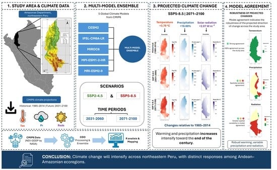
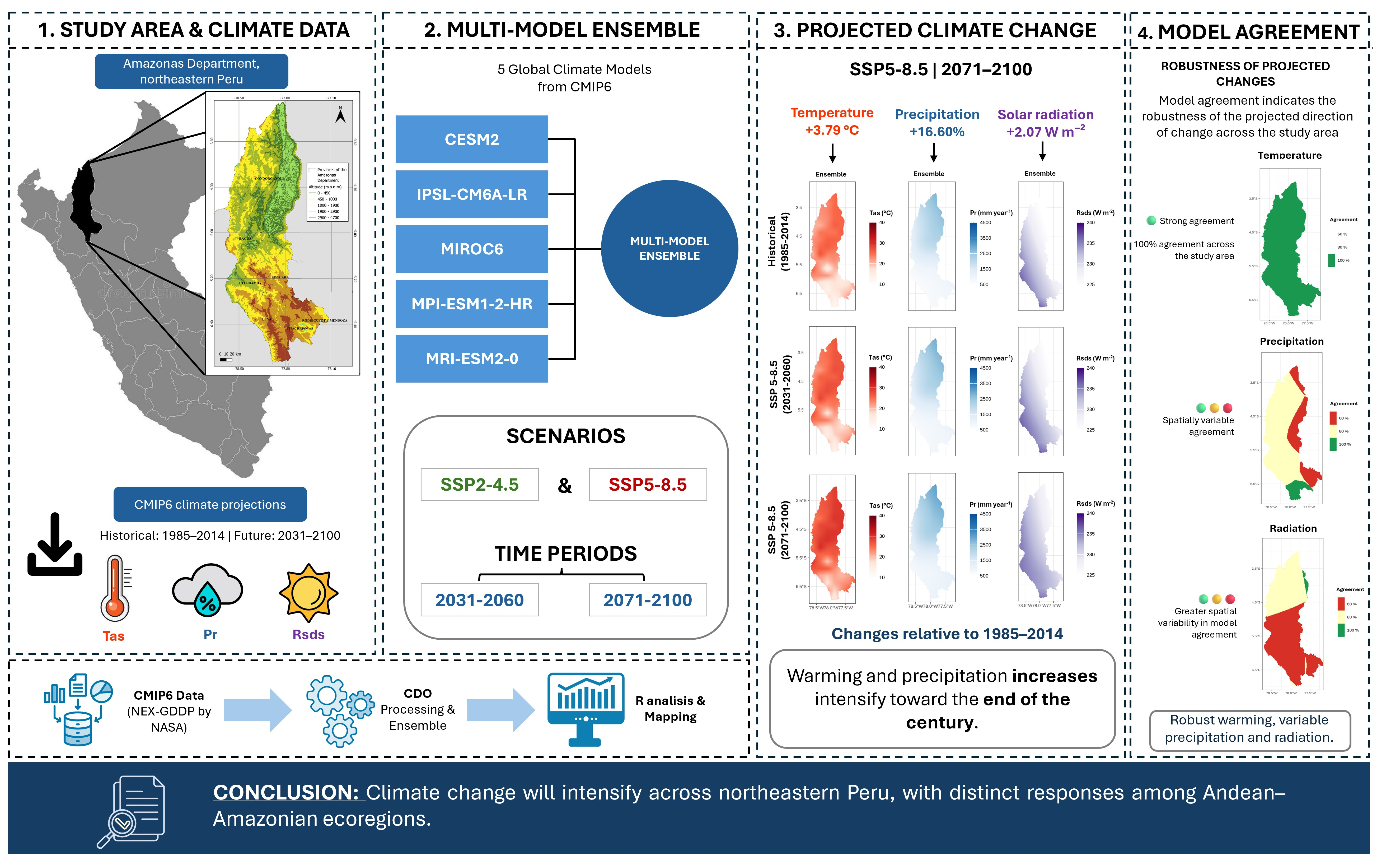
Graphical Abstract

1. Introduction

The alteration of climate systems as a consequence of global warming and anthropogenic activities has led to the development of methods to project changes such as increases in mean temperature, variations in precipitation patterns, and intensification of the hydrological cycle [1,2,3]. South America is one of the world’s most climatically diverse regions, characterized by the interaction of the South American monsoon, tropical circulation, and the complex topography of the Andes Mountains. This interaction produces strong spatial gradients in climatic conditions such as temperature, precipitation, and solar radiation [4,5,6]. These characteristics result in spatially variable responses to climate change, including increasing temperatures and changes in precipitation and seasonality, with particularly important consequences for the Amazon basin and the tropical Andes [7,8].
The Andean–Amazonian region of northern Peru, which includes the department of Amazonas, represents a transition between Andean altitudinal gradients and the Amazon rainforest [9,10]. The region supports high biodiversity and rural populations that depend on ecosystem services [11,12], making information on future climatic changes relevant for regional planning. While CMIP6 models reproduce several large-scale climate features over South America, their performance varies among models, climatic variables, and regions, particularly in areas with complex topography such as the Andes [1,13,14,15]. This has encouraged the use of bias-corrected and statistically downscaled products, such as NEX-GDDP-CMIP6, which provide climate projections at a finer spatial resolution than the native GCM outputs and have been applied to evaluate changes in hydrology and water balance in Amazonian regions [8,13].
However, significant gaps remain in the integrated assessment of multiple climate variables, particularly air temperature, precipitation, and incident shortwave solar radiation, at regional and ecoregional scales in the Andean–Amazonian transition zone. Although bias-corrected and statistically downscaled CMIP6 climate projections are increasingly available for South America, most studies in Peru, Ecuador, and Colombia have focused primarily on temperature and precipitation at national or biome-wide scales [10,16,17], limiting the information available to compare climate responses between the Andean–Amazonian ecoregions under future climate scenarios [1,16,17]. Recent assessments have also shown relevant differences in model performance and uncertainty in the Amazonian and Andean regions, highlighting the importance of multimodel approaches when assessing climate change in areas characterized by complex topography [14,18,19].
To address these knowledge gaps, this study uses historical climate simulations and future projections from the NEX-GDDP-CMIP6 dataset to assess spatial climate variability and projected changes across the Amazonas department. A historical baseline (1985–2014) and two future 30-year periods (2031–2060 and 2071–2100) under the SSP2-4.5 and SSP5-8.5 scenarios were analyzed to characterize projected changes in annual mean air temperature, annual accumulated precipitation, and incoming shortwave solar radiation, as well as their spatial variability among Andean–Amazonian ecoregions. The central objective is to quantify and compare projected climatic changes at the ecoregional level and identify their spatial patterns across the study area.
This study provides a spatially explicit assessment of projected climate change across Andean–Amazonian ecoregions in northern Peru, where ecoregion-specific climate assessments remain limited. By comparing projected changes in temperature, precipitation, and incoming shortwave solar radiation across contrasting ecoregions, the study provides climate information relevant to regional adaptation, ecosystem conservation, and land management. In the context of landscape restoration, differences in projected climatic conditions among ecoregions may also help identify areas where future climate should be considered in restoration planning.

2. Materials and Methods

2.1. Study Area

The study focused on the Amazonas department, located in northeastern Peru. This department is part of a region with great environmental diversity due to its geographic location and altitudinal gradient, ranging from low-lying areas in the Amazon to the higher elevations of the Andean slopes, thus forming an Andean–Amazonian transition zone. Within the department, three main ecoregions were considered: Tropical and Subtropical Humid Broadleaf Forests (TSHBF), Tropical and Subtropical Dry Broadleaf Forests (TSDBF), and Montane Grasslands and Shrublands (MGS). These ecoregions cover approximately 35,766.63, 3055.62, and 431.78 km2, respectively. The ecoregion shapefiles were obtained from the official spatial data platform of the National Service of Natural Areas Protected by the State (SERNANP, Peru) and were spatially clipped to the boundary of the Amazonas department for subsequent analyses. The geographical location, topographic characteristics, and spatial distribution of the ecoregions considered in this study are shown in Figure 1.

2.2. Climate Data

Historical climate simulations and future projections were obtained from the NASA Earth Exchange Global Daily Downscaled Projections (NEX-GDDP-CMIP6, version 2.0) dataset [5,13,18,20]. The historical baseline covered 1985–2014, while future projections were analyzed for 2031–2060 and 2071–2100 under the SSP2-4.5 and SSP5-8.5 scenarios. These scenarios were selected to represent contrasting levels of future radiative forcing: SSP2-4.5 represents an intermediate forcing pathway, whereas SSP5-8.5 represents a high-forcing pathway. Their inclusion allows the magnitude and spatial distribution of projected climate changes to be compared under two contrasting future forcing conditions. Thirty-year periods were used to represent climatological conditions while reducing the influence of interannual variability. The 1985–2014 period was selected as the historical reference because it corresponds to the final 30 years of the NEX-GDDP-CMIP6 historical simulations, whereas 2031–2060 and 2071–2100 were used to represent mid- and late-century future conditions, respectively. NEX-GDDP-CMIP6 provides bias-corrected and statistically downscaled daily climate data at a horizontal resolution of 0.25°. The NEX-GDDP-CMIP6 version 2.0 variables analyzed in this study were near-surface air temperature (tas), precipitation (pr), and incoming shortwave solar radiation (rsds). Daily temperature and solar radiation were averaged to obtain annual mean values, whereas daily precipitation was accumulated to obtain annual totals. Annual values were then averaged over each 30-year period (Table S1).
The characteristics of the selected CMIP6 global climate models are summarized in Table 1.

2.3. Climate Model Selection

The five GCMs used in this study were CESM2, IPSL-CM6A-LR, MIROC6, MPI-ESM1-2-HR, and MRI-ESM2-0. Model selection was based primarily on the joint availability of the three climatic variables (tas, pr, and rsds) and scenarios (SSP2-4.5 and SSP5-8.5) analyzed in the NEX-GDDP-CMIP6 dataset. Previous evaluations of CMIP6 models over South America, Brazil, and the Amazon Basin were also considered to provide regional context for the selected models [14,26], but no formal performance ranking was applied during model selection. Previous studies have shown that the performance of individual GCMs varies according to region, climatic variable, season, and evaluation metric, while several of the models selected here have shown suitable performance in representing temperature and/or precipitation patterns in tropical South America [5,14,18,26,27]. Therefore, the selected models were not assumed to be uniformly superior across all variables or regions, but were used as a five-model ensemble to represent a range of CMIP6 simulations relevant to the study region. The selected models were combined using an equal-weight arithmetic multi-model mean. For each grid cell, climatic variable, scenario, and period, the ensemble mean was calculated as:
X ¯ = 1 n i = 1 n X i
where X ¯ is the ensemble mean, X i is the climatic value from the i-th climate model, and n is the number of models included in the ensemble ( n = 5 ). The resulting multi-model mean therefore represents the selected five-model ensemble rather than the full range of CMIP6 models (Tables S3 and S4). For the late-century SSP5-8.5 scenario (2071–2100), inter-model variability was further characterized using the projected changes from the five individual GCMs [28,29,30]. At each grid cell, inter-model dispersion was calculated as the standard deviation of the model-specific changes, while directional agreement was expressed as the percentage of models showing the same sign of change as the five-model mean.

2.4. Climate Data Processing

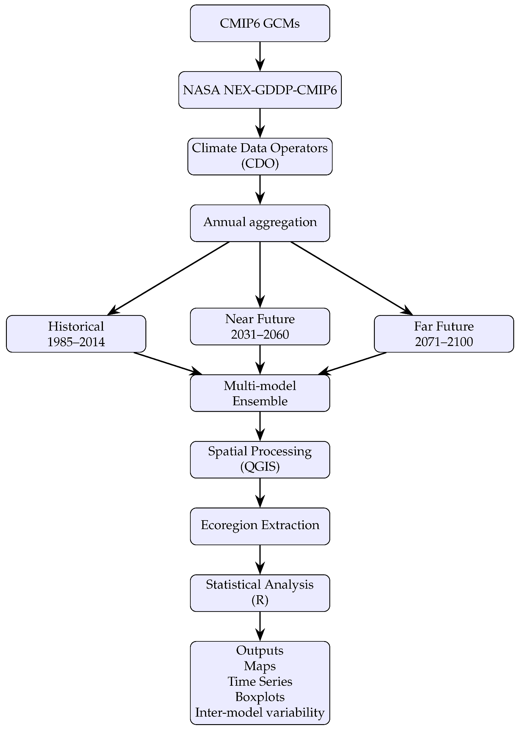
The overall workflow adopted for climate data acquisition, processing, spatial analysis, and visualization is summarized in Figure 2. The workflow illustrates the sequence of procedures applied from the acquisition of NEX-GDDP-CMIP6 climate projections to the generation of multi-model ensembles, ecoregional analyses, and final climatic products. Daily climate series were obtained from the NASA NEX-GDDP-CMIP6 dataset [20] and processed using Climate Data Operators (CDO v2.6.1). Near-surface air temperature (tas) and incoming shortwave solar radiation (rsds) were averaged to obtain annual mean values, while daily precipitation (pr) was accumulated to calculate annual precipitation totals. Annual values were then averaged for the historical (1985–2014), mid-century (2031–2060), and late-century (2071–2100) periods.
For spatial alignment with the study-area grid, the NEX-GDDP-CMIP6 data were bilinearly remapped from their 0.25° grid to a common 0.01° analysis grid. This interpolation was performed for spatial alignment and does not increase the effective spatial resolution of the original climate data.
The resulting multi-model ensemble rasters for each climate variable, scenario, and period were spatially masked to the boundary of the Amazonas department using QGIS v3.38.0. Subsequently, raster values for each ecoregion were extracted using polygon overlay for the calculation of ecoregional means and spatial variability.
All analyses were performed using R version 4.4.3 within a Conda environment on Ubuntu 24.04 LTS, from the command line (Rscript), using the R packages terra (v1.9-34), sf (v1.1-1), tidyterra (v1.2.0), ggplot2 (v4.0.3), dplyr (v1.2.1), and patchwork (v1.3.2). These procedures generated the climate maps, time evolution graphs, ecoregional summaries, inter-model variability analyses, and historical climate evaluation presented in this study.

2.5. Historical Climate Evaluation

Historical climate fields from the five NEX-GDDP-CMIP6 models and their multi-model ensemble were evaluated against the CHELSA v2.1 gridded climate dataset for the common 1985–2014 period [31,32]. The comparison included near-surface air temperature, annual precipitation, and incoming shortwave solar radiation. Because CHELSA and NEX-GDDP-CMIP6 have different spatial resolutions, both datasets were evaluated on a common 0.25° grid. The processed NEX-GDDP-CMIP6 fields were aggregated to this spatial support, while CHELSA data were spatially averaged to the same grid. Similar common-grid approaches have been used when evaluating NEX-GDDP-CMIP6 and other gridded climate products against reference datasets [30,31,33] (Table S2 and Figure S1).
For CHELSA, monthly temperature and incoming shortwave solar radiation values were averaged using the number of days in each month as temporal weights, whereas monthly precipitation was summed to obtain annual precipitation totals. Annual values were subsequently averaged over 1985–2014. Model performance was assessed separately for each GCM and for the arithmetic multi-model ensemble using area-weighted mean bias, mean absolute error (MAE), root mean square error (RMSE), and the area-weighted spatial Pearson correlation coefficient [30,34]. Grid-cell areas within the Amazonas department were used as weights to account for differences in cell area and partial coverage along the department boundary.

2.6. Climate Change Analysis

Future climate conditions for 2031–2060 and 2071–2100 were compared with the historical baseline (1985–2014). Absolute changes in near-surface air temperature (tas) and incoming shortwave solar radiation (rsds) were calculated as the difference between future and historical conditions (Equations (2) and (3), respectively). For precipitation (pr), both absolute changes (mm yr−1) and relative changes (%) were calculated to describe changes in annual precipitation with respect to the historical baseline (Equations (4) and (5), respectively) [35,36,37].
Δ T a s = T a s f u t u r e T a s h i s t o r i c a l
where Δ T a s is the projected temperature change (°C), T a s f u t u r e represents the future annual mean temperature, and T a s h i s t o r i c a l corresponds to the historical baseline.
Δ R s d s = R s d s f u t u r e R s d s h i s t o r i c a l
where Δ R s d s is the projected change in annual mean incoming shortwave solar radiation (W m−2).
Δ P r a b s = P r f u t u r e P r h i s t o r i c a l
where Δ P r a b s is the absolute change in annual precipitation (mm yr−1), P r f u t u r e represents future annual precipitation, and P r h i s t o r i c a l represents annual precipitation during the historical baseline.
Δ P r r e l ( % ) = P r f u t u r e P r h i s t o r i c a l P r h i s t o r i c a l × 100
where Δ P r r e l represents the relative change in annual precipitation (%) with respect to the historical baseline.

2.7. Ecoregional Analysis

Climate conditions and projected changes were summarized separately for the three ecoregions considered in the Amazonas department (TSHBF, TSDBF, and MGS). For each ecoregion, raster values were extracted from the common 0.01° analysis grid obtained by bilinear interpolation of the original 0.25° NEX-GDDP-CMIP6 data. The resulting spatial summaries included 58,336 grid cells for TSHBF, 4988 for TSDBF, and 706 for MGS. At the native NEX-GDDP-CMIP6 resolution of 0.25°, these correspond to approximately 93, 8, and 1 effective climate grid cells for TSHBF, TSDBF, and MGS, respectively, indicating that the ecoregional summaries for TSDBF and especially MGS reflect the climate signal of very few independent grid cells at the original model resolution. Mean climatic conditions were calculated as the arithmetic mean of the raster cell values (Equation (6)), while the sample standard deviation was used to describe spatial variability within each ecoregion (Equation (7)).
X ¯ e c o = 1 m j = 1 m X j
where X ¯ e c o is the mean climatic value for each ecoregion, X j is the climatic value of each raster cell, and m is the total number of cells from the 0.01° analysis grid included within the corresponding ecoregion.
S D e c o = j = 1 m ( X j X ¯ e c o ) 2 m 1
where S D e c o represents the spatial standard deviation of climatic values within each ecoregion. Ecoregional statistics were used descriptively to characterize spatial differences in historical climate conditions and projected changes among TSHBF, TSDBF, and MGS. The standard deviation represents spatial heterogeneity within each ecoregion, whereas inter-model variability was evaluated separately from the individual GCM projections.

2.8. Climate Hotspots

Climate hotspots were identified under SSP5-8.5 for 2071–2100 relative to the historical baseline (1985–2014). This combination represents the highest-forcing and late-century condition evaluated in this study and was used to examine the spatial concentration of the largest projected climatic changes across the Amazonas department. For temperature and incoming shortwave solar radiation, hotspots were based on absolute projected changes, whereas for precipitation they were based on relative changes (%).
For each climatic variable, the 75th percentile ( P 75 ) of projected change was calculated from all valid grid cells across the study area. Grid cells with projected changes equal to or greater than the corresponding P 75 threshold were classified as hotspots (Equation (8)).
H o t s p o t = 1 , Δ X P 75 0 , Δ X < P 75
where Δ X represents the projected change in the climatic variable and P 75 is the corresponding 75th-percentile threshold calculated across the Amazonas department. Hotspot extent within each ecoregion was subsequently quantified as the percentage of its represented area classified as hotspot.

3. Results

3.1. Historical Climate Evaluation

The historical climate fields showed different levels of agreement with CHELSA v2.1 among the three analyzed variables (Table 2). Near-surface air temperature showed the strongest spatial correspondence, with an area-weighted Pearson correlation coefficient of 0.943 for the multi-model ensemble. However, the ensemble showed a positive mean bias of 2.04 °C. Individual GCMs showed similarly high spatial correlations (0.942–0.944), with mean biases ranging from 1.52 to 2.35 °C.
Precipitation showed a moderate spatial correspondence with CHELSA ( r = 0.660 ). The multi-model ensemble underestimated mean annual precipitation by 416.3 mm yr−1, and all individual GCMs showed a negative mean bias, ranging from approximately 453 to −380 mm yr−1. Incoming shortwave solar radiation showed the lowest spatial correspondence ( r = 0.321 ), with a positive mean bias of 31.86 W m−2. Overall, the historical evaluation showed that model performance differed among climatic variables, with stronger spatial agreement for temperature than for precipitation and solar radiation.

3.2. Temporal Evolution of Projected Climate

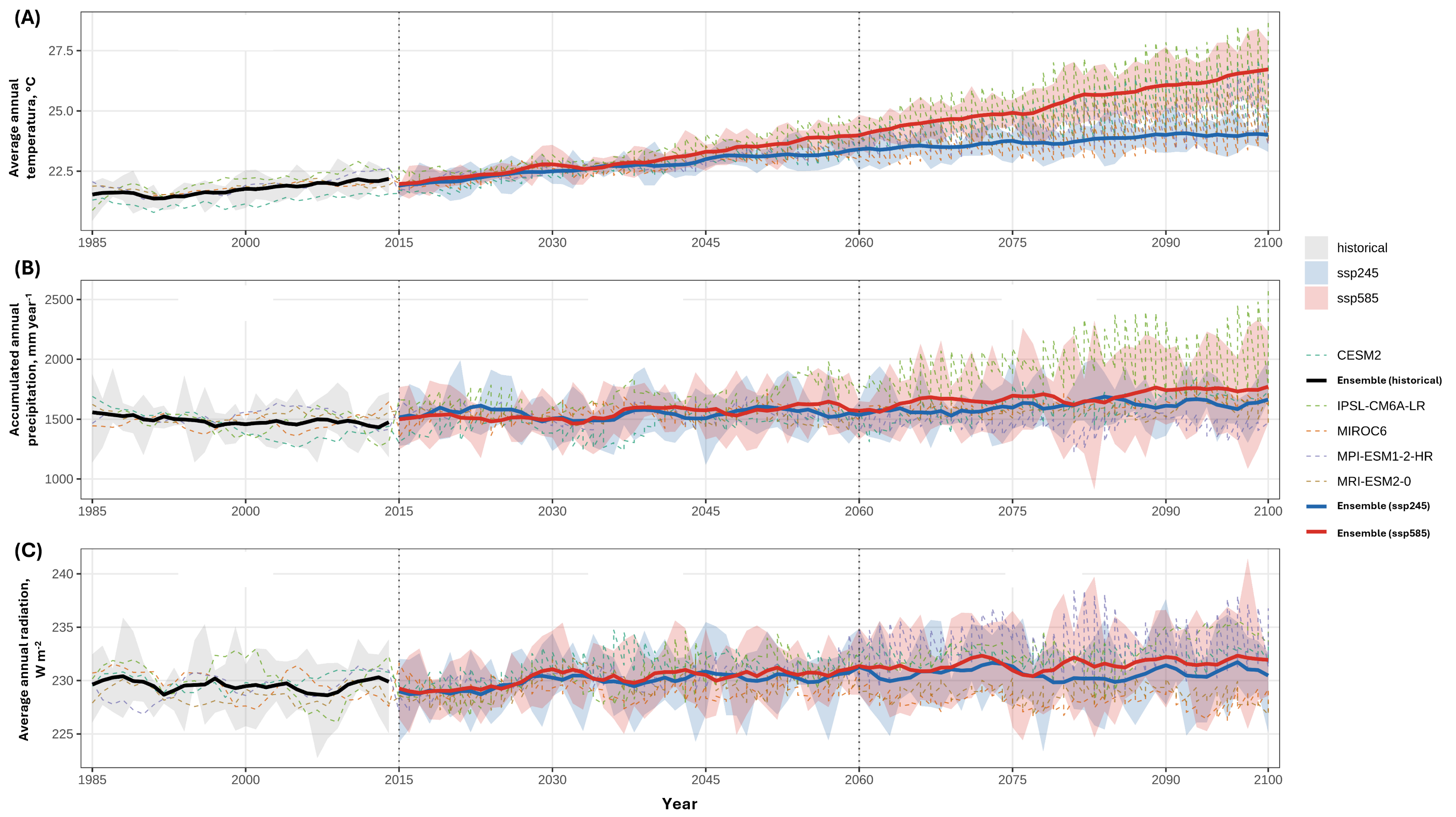
The temporal evolution of mean annual temperature, accumulated annual precipitation, and incoming shortwave solar radiation from the historical period (1985–2014) to the end of the 21st century is presented in Figure 3.
The multi-model ensemble shows a progressive increase in annual mean temperature under both future scenarios, with a larger separation between SSP2-4.5 and SSP5-8.5 toward the end of the century (Figure 3A). The historical mean temperature for 1985–2014 was 21.75 °C. During 2031–2060, mean temperature increased to 22.96 °C under SSP2-4.5 and 23.29 °C under SSP5-8.5, corresponding to increases of 1.20 and 1.53 °C relative to the historical baseline. During 2071–2100, projected mean temperature reached 23.87 °C under SSP2-4.5 and 25.72 °C under SSP5-8.5, with respective increases of 2.12 and 3.96 °C.
Annual precipitation showed greater temporal and inter-model variability than temperature (Figure 3B). The historical multi-model mean was 1486.04 mm yr−1. During 2031–2060, projected mean annual precipitation increased to 1542.90 mm yr−1 under SSP2-4.5 and 1570.10 mm yr−1 under SSP5-8.5. During 2071–2100, the corresponding values increased to 1627.31 and 1709.54 mm yr−1. These changes represent absolute increases of 56.86, 84.06, 141.27, and 223.50 mm yr−1 relative to the historical baseline for SSP2-4.5 and SSP5-8.5 during the two future periods, respectively.
Incoming shortwave solar radiation showed smaller projected changes over time (Figure 3C). The historical multi-model mean was 229.56 W m−2. During 2031–2060, projected values increased to 230.31 W m−2 under SSP2-4.5 and 230.63 W m−2 under SSP5-8.5, corresponding to increases of 0.75 and 1.07 W m−2 relative to the historical baseline. During 2071–2100, mean values reached 230.73 and 231.63 W m−2, corresponding to increases of 1.17 and 2.07 W m−2, respectively.
Overall, the temporal evolution of the projections shows that temperature exhibited the clearest and most consistent increase among the three climatic variables. Precipitation also increased under both scenarios, but with greater temporal and inter-model variability, whereas changes in incoming shortwave solar radiation were comparatively small.

3.3. Spatial Distribution of Projected Climate

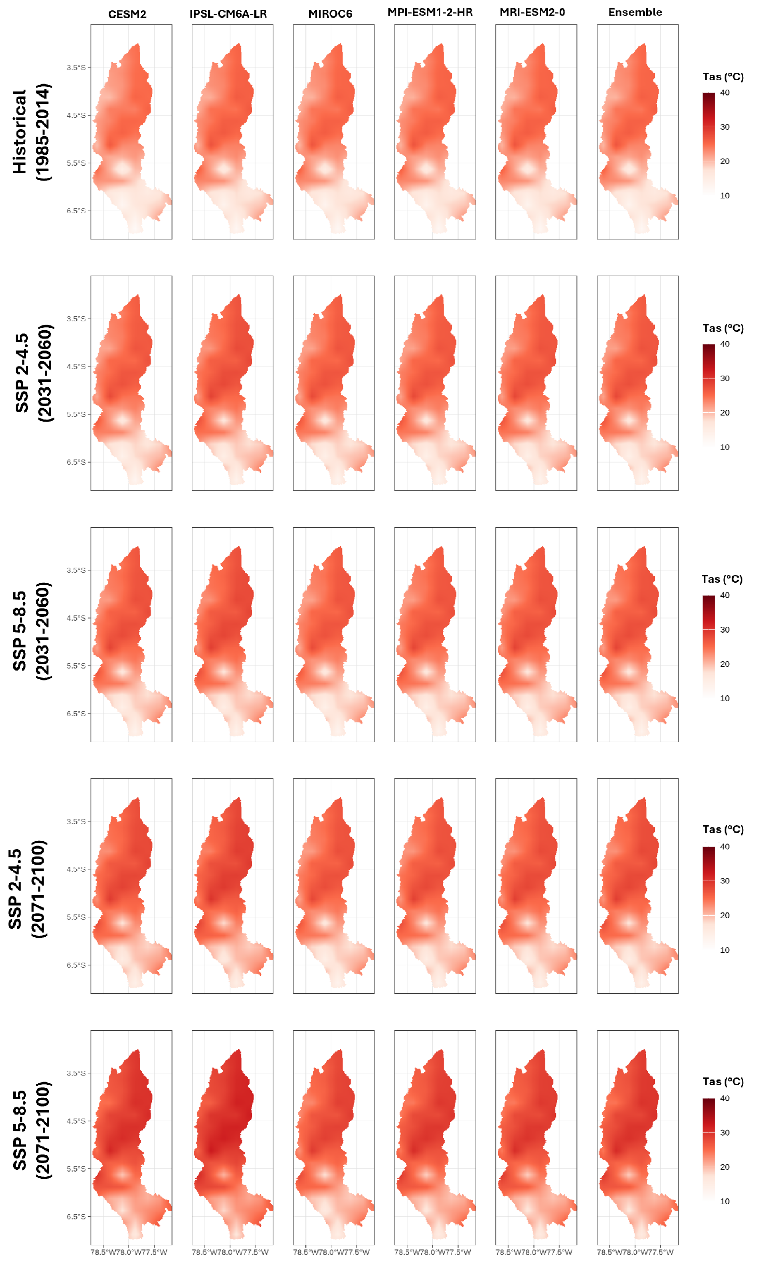
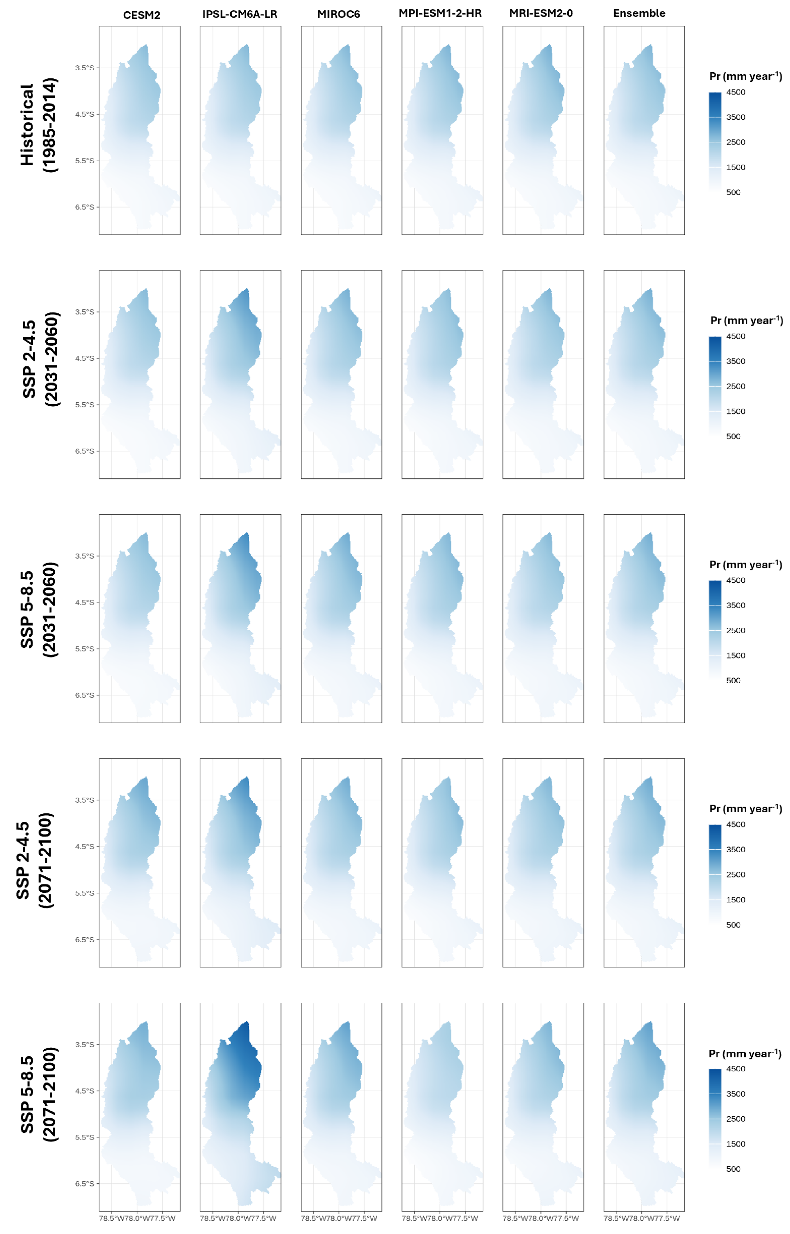
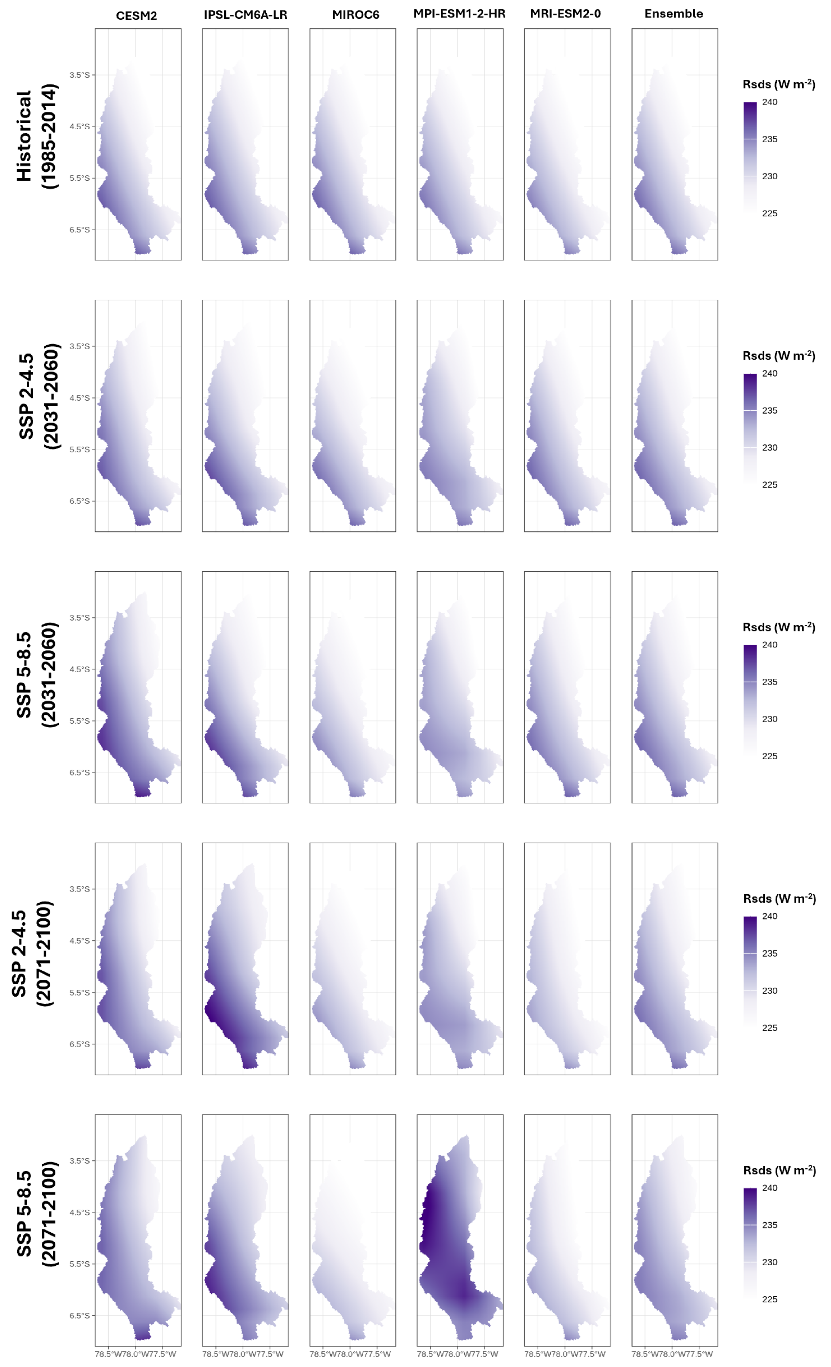
The spatial distribution of mean annual temperature, annual accumulated precipitation, and incoming shortwave solar radiation for the historical period (1985–2014) and the future periods (2031–2060 and 2071–2100) under SSP2-4.5 and SSP5-8.5 is presented in Figure 4, Figure 5 and Figure 6. The historical climate fields showed marked spatial differences across the Amazonas department, and the main spatial patterns were generally maintained in the future projections, although their magnitude differed among scenarios and models.
During the historical period, mean annual temperature showed a clear spatial gradient (Figure 4). The highest temperatures occurred mainly in the northern and northeastern lowland areas of the department, where values exceeded 28 °C in some locations. Lower temperatures occurred toward the southern and southwestern mountainous areas, which also include the higher-elevation sectors shown in Figure 1.
During 2031–2060, higher temperatures were projected throughout the study area under both scenarios, while the historical spatial gradient remained visible. The increases were larger under SSP5-8.5 than under SSP2-4.5. This difference became more pronounced during 2071–2100, when SSP5-8.5 produced the highest projected temperatures. Under this scenario, temperatures exceeded 30 °C across parts of the northern and northeastern lowlands, whereas the southern and southwestern mountainous areas remained comparatively cooler. Although the magnitude of projected temperature differed among the individual GCMs, the main spatial distribution was retained across the future periods. Annual accumulated precipitation also showed pronounced spatial heterogeneity across the department (Figure 5). During the historical period, the highest precipitation values occurred mainly in the northern and northeastern sectors, with values exceeding 3000 mm yr−1 in some areas. In contrast, substantially lower precipitation occurred in parts of the southern and southwestern sectors of the department.
Future projections generally maintained the historical spatial distribution of precipitation, but with increases in accumulated annual precipitation across much of the study area. The increases were larger during 2071–2100, particularly under SSP5-8.5. Differences among individual GCMs were more evident for precipitation than for temperature. IPSL-CM6A-LR projected comparatively high precipitation in parts of the northern sector under late-century SSP5-8.5, whereas other models showed smaller increases. The multi-model ensemble retained the broad historical precipitation pattern while showing higher accumulated precipitation under the future scenarios.
Incoming shortwave solar radiation showed a different spatial distribution from precipitation (Figure 6). During the historical period, higher radiation values occurred mainly in the southern and southwestern sectors of the department, whereas lower values were observed across much of the northern and northeastern areas. Historical values generally ranged around 228–236 W m−2 across much of the study area.
Projected changes in incoming shortwave solar radiation were smaller than those observed for temperature and precipitation. During 2031–2060, both scenarios showed relatively small changes while maintaining the historical spatial pattern. During 2071–2100, SSP5-8.5 generally produced higher radiation values than SSP2-4.5, although the magnitude and spatial distribution of the changes differed among the individual GCMs. The multi-model ensemble showed modest increases across much of the department while retaining the main historical spatial pattern.

3.4. Spatial Climate Anomalies

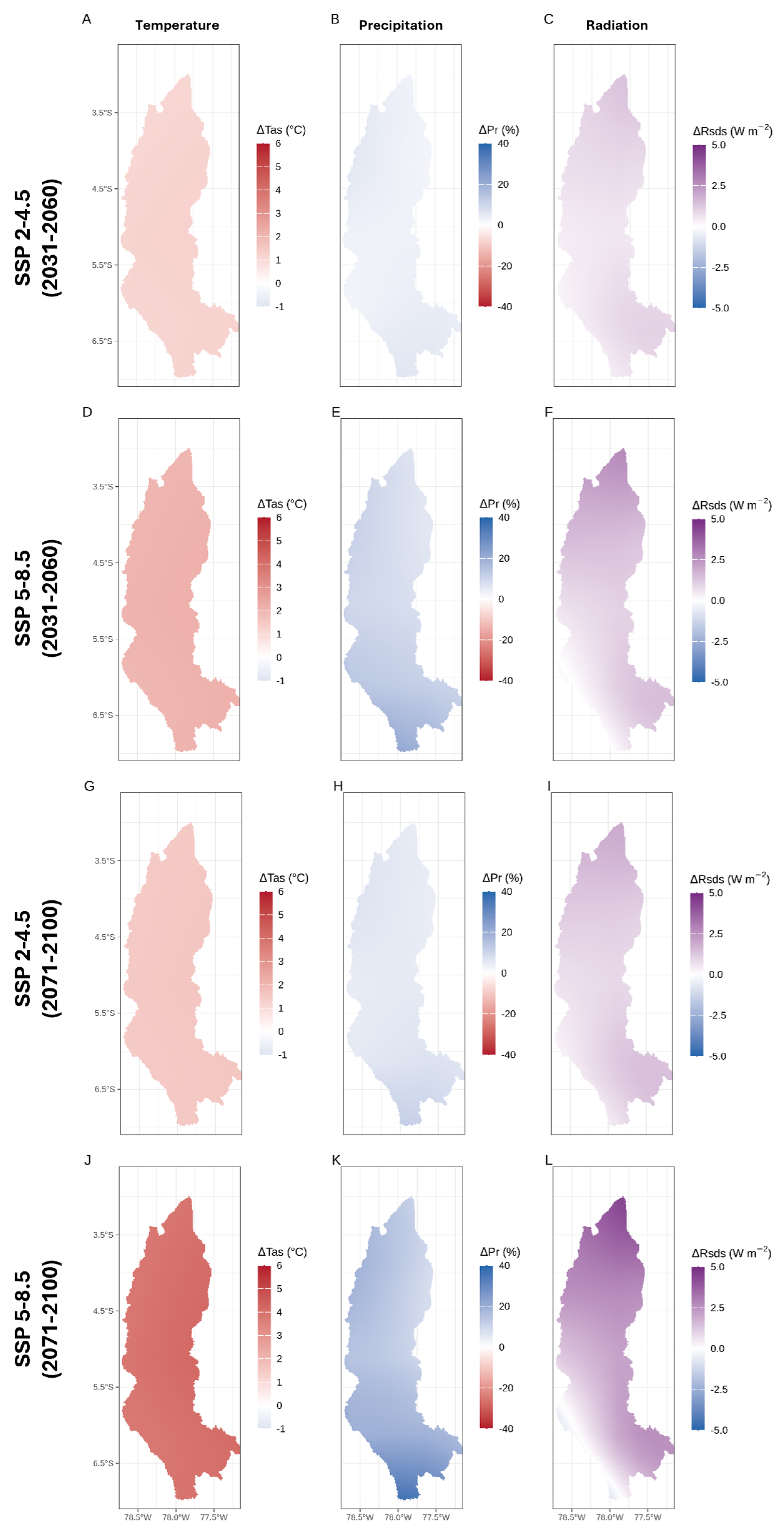
Spatial anomalies of annual mean temperature ( Δ Tas), annual precipitation ( Δ Pr), and incoming shortwave solar radiation ( Δ Rsds) relative to the historical baseline (1985–2014) are presented in Figure 7, whereas the corresponding spatial mean values are summarized in Table 3.
Annual mean temperature showed positive anomalies throughout the Amazonas department under both scenarios and future periods (Figure 7A,D,G,J). During 2031–2060, the mean temperature increase was 1.20 °C under SSP2-4.5 and 1.53 °C under SSP5-8.5. During 2071–2100, the projected increase reached 2.12 °C under SSP2-4.5 and 3.96 °C under SSP5-8.5. Temperature anomalies were comparatively homogeneous across the study area, although their magnitude increased between the two future periods and was larger under SSP5-8.5.
Projected precipitation changes were also predominantly positive across Amazonas (Figure 7B,E,H,K), but their spatial distribution was more heterogeneous than that of temperature. During 2031–2060, mean annual precipitation increased by 56.86 mm yr−1 under SSP2-4.5 and 84.06 mm yr−1 under SSP5-8.5 relative to the historical baseline. During 2071–2100, the corresponding increases reached 141.27 and 223.50 mm yr−1. The mean cellwise relative changes were 3.93% and 5.97% during 2031–2060 and 10.52% and 16.59% during 2071–2100 under SSP2-4.5 and SSP5-8.5, respectively. The largest relative precipitation increases occurred mainly in the southern portion of the department, whereas smaller relative changes occurred across much of the northern sector.
Incoming shortwave solar radiation showed smaller anomalies than the other climatic variables (Figure 7C,F,I,L). During 2031–2060, mean Δ Rsds was 0.75 W m−2 under SSP2-4.5 and 1.07 W m−2 under SSP5-8.5. During 2071–2100, the corresponding mean changes increased to 1.17 and 2.07 W m−2. Under late-century SSP5-8.5, spatial anomalies ranged from approximately 0.73 to 4.41 W m−2, indicating that the department-wide positive mean included localized areas with small negative changes.
Overall, the magnitude of the projected changes increased from 2031–2060 to 2071–2100 and was larger under SSP5-8.5 than under SSP2-4.5. Temperature changes were comparatively homogeneous across Amazonas, whereas precipitation showed greater spatial heterogeneity. Incoming shortwave solar radiation showed relatively small mean changes, although the spatial range widened under late-century SSP5-8.5.

3.5. Climate Variability Among Ecoregions

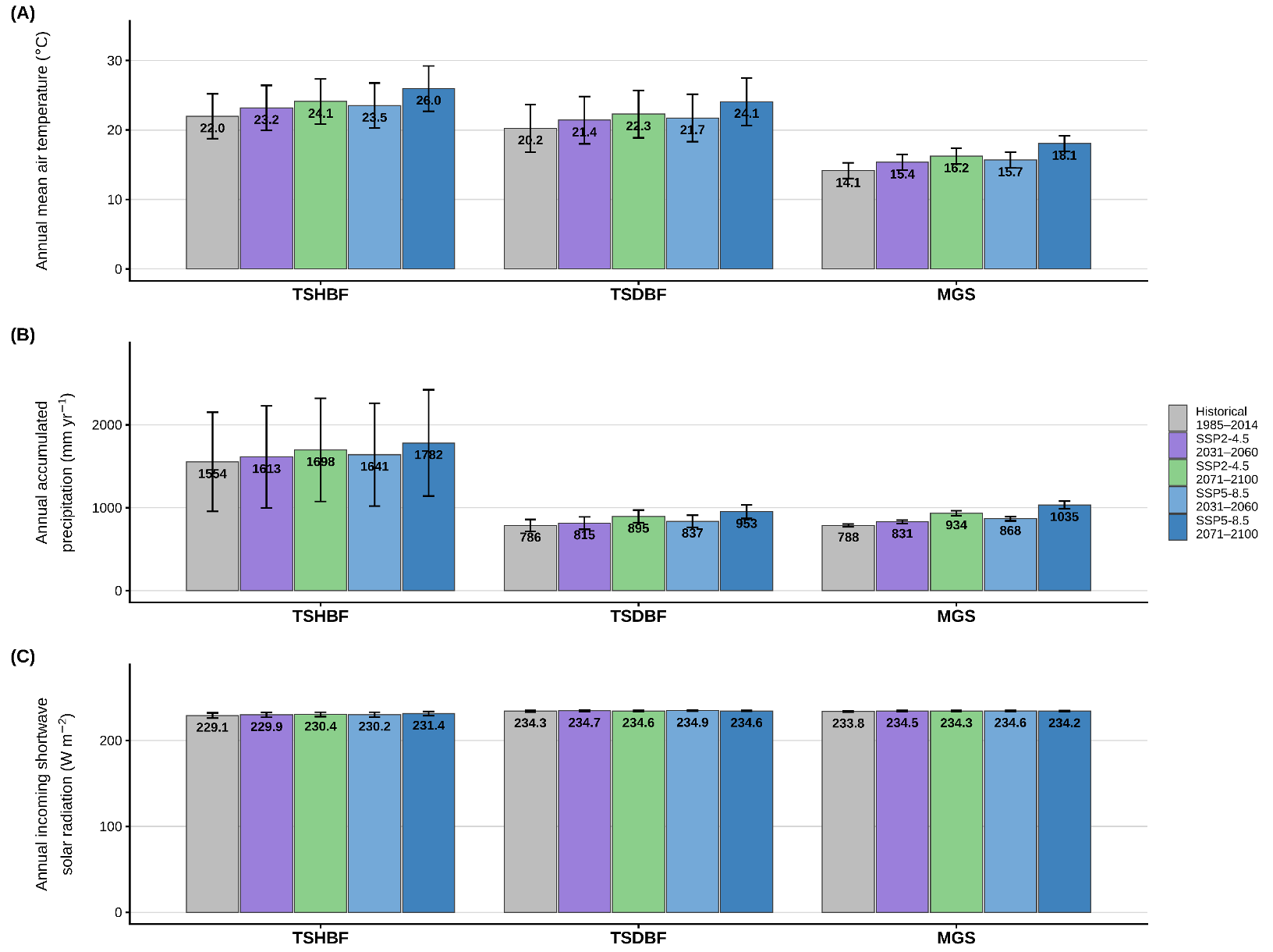
Climatic conditions differed among the three ecoregions throughout the historical and future periods (Figure 8) (Tables S5 and S6). Tropical and Subtropical Humid Broadleaf Forests (TSHBF) showed the highest mean annual temperatures, whereas Montane Grasslands and Shrublands (MGS) showed the lowest. Under SSP5-8.5 during 2071–2100, mean temperature increased by 3.98 °C in TSHBF, 3.84 °C in TSDBF, and 3.91 °C in MGS relative to the historical baseline. The relative ordering of mean temperature among ecoregions was maintained across all analyzed periods.
Annual precipitation increased across the three ecoregions, although the magnitude of the projected change differed among them (Figure 8B). TSHBF remained the wettest ecoregion, increasing from 1553.98 mm yr−1 during 1985–2014 to 1781.98 mm yr−1 under SSP5-8.5 during 2071–2100. Over the same periods, mean annual precipitation increased from 786.46 to 953.23 mm yr−1 in TSDBF and from 787.77 to 1034.68 mm yr−1 in MGS. The corresponding mean relative increases under late-century SSP5-8.5 were 16.00% in TSHBF, 21.36% in TSDBF, and 31.28% in MGS, with MGS showing the largest relative precipitation increase among the three ecoregions. However, this result should be interpreted with caution because MGS corresponds to approximately one effective 0.25° climate grid cell at the native NEX-GDDP-CMIP6 resolution. Therefore, the 31.28% value should be regarded as an indicative estimate for this small ecoregion rather than as a spatially well-resolved ecoregional average.
Incoming shortwave solar radiation showed smaller changes among periods and scenarios (Figure 8C). Under SSP5-8.5 during 2071–2100, mean radiation increased by 2.24 W m−2 in TSHBF, 0.32 W m−2 in TSDBF, and 0.44 W m−2 in MGS relative to the historical baseline. TSHBF therefore showed a larger absolute increase in solar radiation than TSDBF and MGS under this scenario and period.
The numerical summaries for each ecoregion are presented in Table 4. The standard deviations describe spatial variability within each ecoregion.
Spatial variability also differed among ecoregions and climatic variables. TSHBF showed the largest spatial standard deviation for precipitation in all analyzed periods, ranging from 596.84 mm yr−1 during the historical period to 640.63 mm yr−1 under SSP5-8.5 during 2071–2100. Temperature also showed greater spatial variability within TSHBF and TSDBF than within MGS. In contrast, incoming shortwave solar radiation showed comparatively small spatial standard deviations, particularly in TSDBF and MGS.

3.6. Climate Hotspots

Climate hotspots under SSP5-8.5 for 2071–2100 showed distinct patterns among the three climatic variables (Table 5). The 75th-percentile thresholds used for hotspot classification were 4.04 °C for annual mean temperature change, 18.59% for relative annual precipitation change, and 2.69 W m−2 for incoming shortwave solar radiation change.
Temperature hotspots occurred only within Tropical and Subtropical Humid Broadleaf Forests (TSHBF), where they represented 27.38% of the ecoregion’s represented area. Precipitation hotspots showed a different distribution, covering 21.56% of TSHBF, 53.77% of Tropical and Subtropical Dry Broadleaf Forests (TSDBF), and 100% of Montane Grasslands and Shrublands (MGS). Incoming shortwave solar radiation hotspots were restricted to TSHBF, where they represented 27.42% of the represented area (Table S7).

3.7. Inter-Model Variability and Directional Agreement

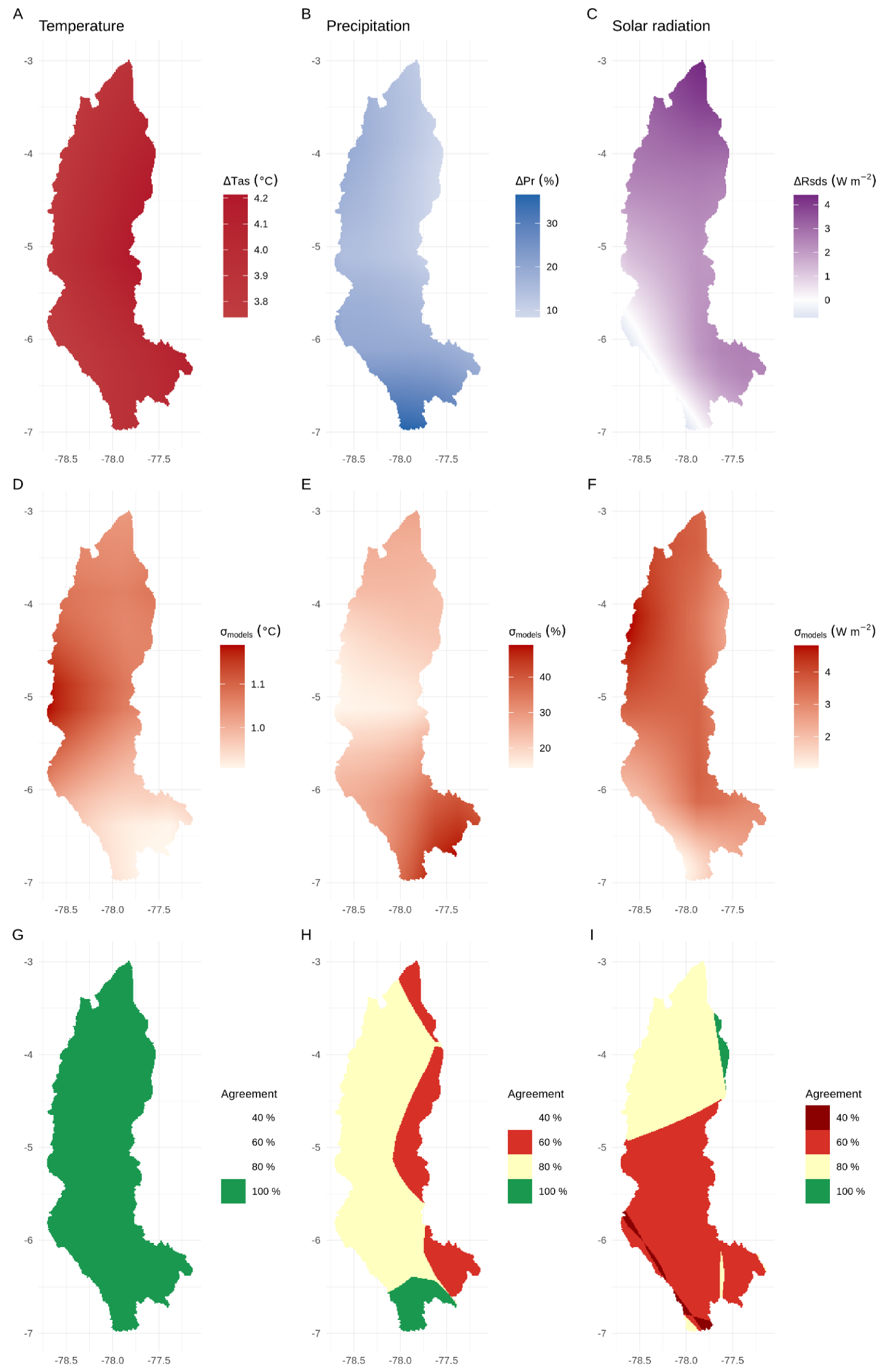
Inter-model variability and directional agreement were evaluated for projected climate changes under SSP5-8.5 during 2071–2100 relative to the historical baseline (1985–2014) (Figure 9). For each climatic variable, the analysis included the multi-model mean projected change, the standard deviation across the five model-specific projected changes, and the percentage of models whose direction of change agreed with the sign of the multi-model mean (Table S8).
Annual mean temperature showed positive projected changes throughout the Amazonas department, ranging from approximately 3.74 to 4.21 °C (Figure 9A). Inter-model standard deviation ranged from approximately 0.91 to 1.19 °C across the study area (Figure 9D). Directional agreement was 100% in all grid cells, indicating that all five models projected temperature changes with the same positive sign as the multi-model mean (Figure 9G).
Projected precipitation changes were predominantly positive but showed greater spatial variation in magnitude than temperature, ranging from approximately 8.40 to 36.62% across the study area (Figure 9B). The standard deviation across the five model-specific precipitation changes ranged from approximately 14.49 to 48.94 percentage points, with the largest values occurring mainly in the southern portion of the department (Figure 9E). Directional agreement was 60% (3 of 5 models) in 22.62% of grid cells, 80% (4 of 5 models) in 70.48%, and 100% (5 of 5 models) in 6.90% of grid cells (Figure 9H).
Incoming shortwave solar radiation showed projected changes ranging from approximately 0.73 to 4.41 W m−2 (Figure 9C). Inter-model standard deviation ranged from approximately 1.03 to 4.82 W m−2 across the study area (Figure 9F). Directional agreement was 40% (2 of 5 models) in 1.81% of grid cells, 60% (3 of 5 models) in 56.15%, 80% (4 of 5 models) in 40.69%, and 100% (5 of 5 models) in 1.35% of grid cells (Figure 9I).
Overall, directional agreement differed among the three climatic variables. Temperature showed 100% agreement across the entire study area, whereas precipitation was dominated by 80% agreement and incoming shortwave solar radiation by 60% agreement. Inter-model variability also differed spatially among the variables, particularly for precipitation and solar radiation.

4. Discussion

4.1. Historical Climate Evaluation

The historical evaluation against CHELSA showed clear differences in performance among the three climatic variables. Annual mean temperature showed the closest spatial correspondence, with a high spatial correlation ( r = 0.943 ), although NEX-GDDP-CMIP6 was warmer by an average of 2.04 °C. Precipitation showed a moderate spatial correlation ( r = 0.660 ) and an average negative bias of 416.32 mm yr−1, indicating larger differences in both the magnitude and spatial representation of rainfall. Incoming shortwave solar radiation showed the lowest spatial correlation ( r = 0.321 ) and a positive mean bias of 31.86 W m−2.
The better spatial representation of temperature compared with precipitation is consistent with previous evaluations of CMIP6-based climate products in Peru and the tropical Andes [13]. Precipitation is generally more difficult to reproduce in this region because its spatial distribution is influenced by complex topography, moisture transport, atmospheric circulation, and local rainfall processes [13,38]. These factors can contribute to substantial differences among climate products, particularly across the Andes–Amazon transition.
The comparison with CHELSA should also be interpreted considering that CHELSA is a gridded climate product rather than a direct set of observations at each model grid cell. Therefore, the evaluation describes the correspondence between two climate datasets and does not represent an independent validation against local weather-station observations. The historical differences between NEX-GDDP-CMIP6 and CHELSA also provide context for interpreting the future projections. Because projected changes were calculated relative to the NEX-GDDP-CMIP6 historical baseline, the reported anomalies describe changes within the same model framework rather than differences relative to CHELSA. Historical differences and projected change should therefore be interpreted separately. Nevertheless, the closer historical correspondence found for temperature provides a stronger basis for interpreting its spatial patterns, whereas the larger differences found for precipitation require greater caution when considering their magnitude and spatial distribution. The low spatial correspondence and positive bias found for incoming shortwave solar radiation similarly limit the level of spatial detail that can be inferred from its projected changes.

4.2. Spatial Distribution of Projected Climate

The spatial patterns of temperature, precipitation, and incoming shortwave solar radiation remained broadly similar between the historical and future periods. Warmer conditions occurred mainly in the northern and northeastern lowlands, while cooler conditions occurred mainly in the mountainous areas of southern and southwestern Amazonas. This spatial contrast broadly follows the topographic gradient of the study area, with higher-elevation terrain concentrated in the southern and southwestern sectors (Figure 1). Future projections mainly showed changes in the magnitude of the climatic variables rather than major shifts in their spatial distribution. This was particularly clear for temperature, which increased throughout the department while maintaining its main historical spatial pattern.
Similar temperature patterns have been reported across the tropical Andes, where climatic conditions vary markedly along elevation gradients [39,40,41]. Precipitation showed a more heterogeneous spatial response. Across the Andes–Amazon transition, rainfall patterns are influenced by the interaction between topography and moisture transport from the Amazon Basin [42,43]. In Amazonas, this spatial complexity remained visible in the future projections: annual precipitation increased on average, but the magnitude of change varied considerably across the department. The lower directional agreement among the five models for precipitation, compared with temperature, also indicates that its future spatial pattern is less consistent across the selected models.
Incoming shortwave solar radiation generally maintained its broad historical spatial pattern in the future projections, although the magnitude and spatial distribution of the projected changes differed among the individual GCMs. The lower directional agreement found for this variable, compared with temperature, indicates that the spatial pattern of future changes was less consistent across the selected models.

4.3. Climate Anomalies

Projected climate anomalies differed among the three climatic variables. Temperature increased throughout the Amazonas department under all scenarios and periods, reaching a mean anomaly of 3.96 °C under SSP5-8.5 during 2071–2100. Warming was also more spatially consistent than the changes projected for precipitation and incoming shortwave solar radiation. A similar contrast has been reported in CMIP6 studies for South America and the tropical Andes, where temperature projections generally show greater spatial consistency and agreement among models than precipitation projections [13,18,26].
Precipitation increased on average, reaching 223.50 mm yr−1, or 16.59%, under SSP5-8.5 during 2071–2100, but the magnitude of change varied considerably across the department. This heterogeneous response is consistent with the complex rainfall patterns of the Andes–Amazon transition, where topography interacts with moisture transport and regional atmospheric circulation [42,43]. These processes can produce major spatial differences in rainfall over relatively short distances. The greater inter-model variability and lower directional agreement found for precipitation in our analysis are also consistent with the wider differences among models reported for precipitation projections in this region [13,26].
Incoming shortwave solar radiation showed smaller absolute changes, with a department-wide mean increase of 2.07 W m−2 under SSP5-8.5 during 2071–2100. However, local changes ranged from 0.73 to 4.41 W m−2, showing that the direction and magnitude of change were not uniform across the study area. Directional agreement among the five models was also lower than for temperature. Because regional CMIP6 evidence for future incoming shortwave solar radiation in the tropical Andes remains limited, these results are best interpreted as a spatially variable response within the selected model ensemble rather than as a general regional pattern.
Overall, the anomalies indicate widespread warming across Amazonas, together with more spatially variable changes in precipitation and incoming shortwave solar radiation. This contrast is important because future climatic conditions across the department will involve changes in several climate variables rather than a uniform response across the region.

4.4. Climate Variability Among Ecoregions

The comparison among ecoregions showed that projected climate change does not have the same magnitude across the Amazonas department. TSHBF remained the warmest and wettest ecoregion throughout the analyzed periods, whereas MGS maintained the lowest mean temperatures. Despite these climatic differences, late-century warming under SSP5-8.5 was relatively similar among ecoregions, reaching 3.98 °C in TSHBF, 3.84 °C in TSDBF, and 3.91 °C in MGS. This suggests that the main temperature differences among ecoregions are maintained even as warming occurs across the department.
A clearer contrast among ecoregions was found for precipitation. TSHBF remained the wettest ecoregion in absolute terms, but MGS showed the largest relative increase, reaching 31.28% under SSP5-8.5 during 2071–2100, compared with 21.36% in TSDBF and 16.00% in TSHBF. The small spatial extent of MGS is important when interpreting this difference, as the ecoregion corresponds to approximately one effective climate grid cell at the native 0.25° resolution. The projected increase therefore indicates a marked precipitation change for the climatic conditions represented within MGS, although finer-scale spatial variability within the ecoregion cannot be resolved with the available data. Rainfall in tropical Andean environments varies strongly with topography and atmospheric moisture transport [44,45], providing a regional context for the differences observed among the three ecoregions. Incoming shortwave solar radiation showed another pattern, with the largest late-century increase occurring in TSHBF, while changes were smaller in TSDBF and MGS. Together, these results show that each ecoregion is exposed to a different combination of projected changes in temperature, precipitation, and solar radiation.
These differences are relevant when climate information is used for ecosystem management. Studies in the Peruvian and tropical Andes have shown that changes in temperature and precipitation can have different effects on montane forests, grasslands, wetlands, and other high-elevation ecosystems [15,46]. Spatial climate information can therefore help identify areas where future conditions may differ from the historical climate and can be combined with information on biodiversity, land use, connectivity, and ecosystem condition to support conservation and restoration planning [15,47]. In this context, the ecoregional differences identified in Amazonas provide a climatic basis for future assessments of ecosystem responses and for the design of adaptation and restoration strategies suited to local conditions.

4.5. Inter-Model Variability and Directional Agreement

The comparison among the five GCMs showed clear differences in inter-model variability and directional agreement among the climatic variables. Temperature had the most consistent response, with all five models projecting warming throughout the Amazonas department under SSP5-8.5 during 2071–2100. In contrast, precipitation and incoming shortwave solar radiation showed lower directional agreement and greater differences in the magnitude of projected change among models. For precipitation, most grid cells showed agreement among four of the five models (80%), whereas solar radiation was dominated by agreement among three of the five models (60%).
The greater agreement for temperature compared with precipitation is consistent with previous CMIP6 studies for South America and the tropical Andes [13,18,26]. Temperature responds strongly to large-scale radiative forcing, whereas precipitation also depends on regional processes such as atmospheric circulation, convection, moisture transport, and interactions with topography. These processes are more difficult to represent consistently across global climate models, particularly in mountainous regions [13,26]. This provides a regional context for the larger differences among precipitation projections found in Amazonas.
Incoming shortwave solar radiation showed a less consistent response among the selected models. Although the multi-model mean indicated a small increase across most of the department, individual models differed in both the magnitude and direction of change. Direct CMIP6 evidence for future incoming shortwave solar radiation in the tropical Andes remains limited, making regional comparisons more difficult.
Overall, the selected models showed a consistent direction of change for temperature, while precipitation and incoming shortwave solar radiation presented greater inter-model variability. This distinction is important when interpreting the projections because agreement in the direction of change does not necessarily imply similar agreement in its magnitude. The multi-model ensemble provides a useful summary of the projected climate response, while the differences among individual models remain relevant when considering future climatic conditions.

4.6. Implications for Landscape Restoration and Ecosystem Resilience

The projected changes identified in this study are relevant for landscape restoration in the Andean–Amazonian transition zone because restoration actions implemented today will develop under climatic conditions that may differ from those of the historical period [48]. Spatial climate projections can help identify these changes and, when combined with ecological and land-use information, support the selection of restoration areas, species, and plant material suited to future conditions [15,47,49]. Climate information can therefore complement, rather than replace, the ecological criteria commonly used in restoration planning.
This approach is particularly relevant in the tropical Andes, where climate exposure and ecosystem responses vary considerably across the landscape. In the Peruvian Andes, projected changes in temperature and precipitation have been used to identify areas where montane forests may experience future climatic conditions outside their current range, providing useful information for conservation prioritization [15]. Climate-informed restoration approaches can also incorporate future climatic suitability into the selection of species and seed sources, reducing reliance on historical climate alone when planning long-term restoration [47].
For Amazonas, the differences found among ecoregions indicate that a single restoration approach may not be suitable across the entire department. Warming was projected throughout the three ecoregions, while precipitation and incoming shortwave solar radiation showed different magnitudes of change. MGS showed the largest relative precipitation increase, whereas TSHBF showed the largest increase in incoming shortwave solar radiation under late-century SSP5-8.5. These differences provide climate information that can be considered when defining restoration objectives and evaluating future conditions at the ecoregional level.
These projections describe future climate exposure and should not be interpreted as direct measures of ecosystem vulnerability or resilience. Assessing resilience requires additional information on vegetation, soils, species responses, landscape connectivity, disturbance, and land-use pressures. Combining these factors with spatial climate projections would provide a more complete basis for identifying restoration priorities and selecting management strategies that remain suitable under changing climatic conditions.
Some aspects of the study design should be considered when interpreting these results. The analysis was based on five equally weighted GCMs, and the multi-model mean may therefore be sensitive to the composition of the selected ensemble, particularly for precipitation, for which larger differences among individual models were observed. Climate models within CMIP6 are also not fully independent because some share components and development histories, which can influence the information represented by multi-model ensembles [28,29]. In addition, although the NEX-GDDP-CMIP6 data were interpolated to a 0.01° grid for spatial analysis, their effective climate resolution remains 0.25°; therefore, the finer grid should not be interpreted as providing additional local climate information, particularly when interpreting local-scale patterns across complex Andean terrain.
Furthermore, the analysis focused on annual mean and annually accumulated climate variables, which may not capture potential changes in the frequency, intensity, or duration of climate extremes such as heatwaves, droughts, or intense precipitation episodes; annual averages may therefore mask important changes in short-term climate variability, and this should be considered when applying these results to ecosystem management and restoration planning. Finally, the historical evaluation relied on CHELSA v2.1 as a reference dataset rather than on direct in situ weather-station observations; the evaluation therefore describes the correspondence between two gridded climate datasets and does not constitute an independent validation against local observations, which remains an important limitation in regions with complex terrain such as the Andes.

5. Conclusions

This study assessed projected changes in annual mean temperature, annual accumulated precipitation, and incoming shortwave solar radiation across the Amazonas department of northeastern Peru using an ensemble of five NEX-GDDP-CMIP6 climate models under the SSP2-4.5 and SSP5-8.5 scenarios. The analysis showed that the magnitude and spatial variability of projected change differed among climatic variables and ecoregions.
Temperature showed the most consistent direction of change among the selected models, with warming projected throughout the department and the largest increases occurring under SSP5-8.5 during 2071–2100. Precipitation also increased on average, but showed greater spatial and inter-model variability, whereas incoming shortwave solar radiation showed less spatially uniform changes. Despite these changes, the main historical spatial patterns of the three climatic variables remained broadly similar in the future projections.
Differences were also evident among ecoregions. Tropical and Subtropical Humid Broadleaf Forests remained the warmest and wettest ecoregion, while Montane Grasslands and Shrublands maintained the lowest mean temperatures and showed the largest relative precipitation increase under late-century SSP5-8.5. The latter pattern should be interpreted at the spatial scale supported by the climate data, given the small extent of MGS relative to the effective 0.25° resolution.
The interpretation of these projections is subject to several limitations. The analysis was based on five equally weighted GCMs and therefore represents the selected ensemble rather than the full range of CMIP6 simulations. The effective climate resolution remained 0.25° despite interpolation to a finer analysis grid, limiting the representation of local-scale climatic variability. Inter-model variability was greater for precipitation and incoming shortwave solar radiation than for temperature. In addition, the historical evaluation was based on comparison with the gridded CHELSA v2.1 dataset rather than direct weather-station observations, and the use of annual climatic variables does not capture seasonal patterns or extreme events.
Overall, the results provide spatially explicit climate information for a region characterized by strong environmental heterogeneity. By combining CMIP6 climate projections with an ecoregion-based assessment, this study provides information that can support climate-informed decision-making, conservation, and landscape restoration planning, and can serve as an input for future assessments of ecosystem responses and resilience in the Andean–Amazonian region.

Supplementary Materials

The following supporting information can be downloaded at https://www.mdpi.com/article/10.3390/land15091745/s1.

Author Contributions

Conceptualization, A.V.C.H. and H.V.V.P.; methodology, A.V.C.H. and D.P.; software, A.V.C.H. and D.P.; validation, A.V.C.H., D.P., E.I.A. and H.V.V.P.; formal analysis, A.V.C.H.; investigation, A.V.C.H.; resources, H.V.V.P.; data curation, A.V.C.H.; writing—original draft preparation, A.V.C.H.; writing—review and editing, D.P., E.I.A. and H.V.V.P.; visualization, A.V.C.H. and D.P.; supervision, H.V.V.P.; project administration, H.V.V.P.; funding acquisition, A.V.C.H. and H.V.V.P. All authors have read and agreed to the published version of the manuscript.

Funding

This research was funded by the National Council for Science, Technology and Technological Innovation (CONCYTEC) and the National Program for Scientific Research and Advanced Studies (PROCIENCIA) under call E077-2023-01-BM “Scholarships for Doctoral Programs in Interinstitutional Alliances”, grant PE501092492-2024, and under call E033-2023-01-BM “Interinstitutional Alliances for Doctoral Programs”, grant PE501084305-2023.

Data Availability Statement

All data generated or analyzed during this study are included in this published article.

Acknowledgments

The authors would like to thank the Doctoral Program in Sciences for Sustainable Development of the Universidad Nacional Toribio Rodríguez de Mendoza de Amazonas. Also, they would like to thank the Consejo Nacional de Ciencia, Tecnología e Innovación Tecnológica (CONCYTEC) and the Programa Nacional de Investigación Científica y Estudios Avanzados (PROCIENCIA) within the framework of the Call E033-2023-01-BM “Interinstitutional Alliances for Doctoral Programs,” under grant number (PE501084305-2023). During the preparation of this manuscript, the authors used ChatGPT (OpenAI; model GPT-5.6) to assist with English-language grammar and style editing. The authors also used Consensus Consensus (Consensus.app 2.0) as an AI-assisted literature discovery tool to support reference searching and cross-checking. All AI-assisted outputs were reviewed and edited by the authors; all references were verified against the original sources. The authors take full responsibility for the content of this publication.

Conflicts of Interest

The authors declare no conflicts of interest. The funders had no role in the design of the study; in the collection, analyses, or interpretation of data; in the writing of the manuscript; or in the decision to publish the results.

Abbreviations

The following abbreviations are used in this manuscript:
CMIP6Coupled Model Intercomparison Project Phase 6
GCMGlobal Climate Model
MMEMulti-Model Ensemble
SSPShared Socioeconomic Pathway
NEX-GDDP-CMIP6NASA Earth Exchange Global Daily Downscaled Projections CMIP6
NASANational Aeronautics and Space Administration
CHELSAClimatologies at High Resolution for the Earth’s Land Surface Areas
CDOClimate Data Operators
QGISQGIS Geographic Information System
SERNANPServicio Nacional de Áreas Naturales Protegidas por el Estado
tasNear-Surface Air Temperature
prPrecipitation
rsdsSurface Downwelling Shortwave Radiation
TSHBFTropical and Subtropical Humid Broadleaf Forests
TSDBFTropical and Subtropical Dry Broadleaf Forests
MGSMontane Grasslands and Shrublands
SDStandard Deviation

References

  1. Marengo, J.; Espinoza, J.C.; Fu, R.; Jimenez Muñoz, J.; Alves, L.; DA ROCHA, H.; Schöngart, J. Long-term variability, extremes and changes in temperature and hydrometeorology in the Amazon region: A review. Acta Amaz. 2024, 54, e54es22098. [Google Scholar] [CrossRef] [Scilit]
  2. Pabón-Caicedo, J.; Arias, P.; Carril, A.; Espinoza, J.; Borrel, L.; Goubanova, K.; Lavado-Casimiro, W.; Masiokas, M.; Solman, S.; Villalba, R. Observed and Projected Hydroclimate Changes in the Andes. Front. Earth Sci. 2020, 8, 61. [Google Scholar] [CrossRef] [Scilit]
  3. Masson-Delmotte, V.; Zhai, P.; Pirani, A.; Connors, S.L.; Péan, C.; Berger, S.; Caud, N.; Chen, Y.; Goldfarb, L.; Gomis, M. Climate change 2021: The physical science basis. Contrib. Work. Group I Sixth Assess. Rep. Intergov. Panel Clim. Change 2021, 2, 2391. [Google Scholar]
  4. Reboita, M.; Kuki, C.; Marrafon, V.; de Souza, C.; Ferreira, G.; Teodoro, T.; Lima, J. South America climate change revealed through climate indices projected by GCMs and Eta-RCM ensembles. Clim. Dyn. 2022, 58, 459–485. [Google Scholar] [CrossRef] [Scilit]
  5. Ortega, G.; Arias, P.; Villegas, J.; Marquet, P.; Nobre, P. Present-day and future climate over central and South America according to CMIP5/CMIP6 models. Int. J. Climatol. 2021, 41, 6713–6735. [Google Scholar] [CrossRef] [Scilit]
  6. Olmo, M.E.; Espinoza, J.; Bettolli, M.L.; Sierra, J.P.; Junquas, C.; Arias, P.; Moron, V.; Balmaceda-Huarte, R. Circulation patterns and associated rainfall over south tropical South America: GCMs evaluation during the dry-to-wet transition season. J. Geophys. Res. Atmos. 2022, 127, e2022JD036468. [Google Scholar] [CrossRef] [Scilit]
  7. Huang, Y.; Xue, M.; Hu, X.; Martin, E.; Novoa, H.M.; McPherson, R.A.; Liu, C.; Chen, M.; Hong, Y.; Perez, A. Increasing frequency and precipitation intensity of convective storms in the Peruvian Central Andes: Projections from convection-permitting regional climate simulations. Q. J. R. Meteorol. Soc. 2024, 150, 4371–4390. [Google Scholar] [CrossRef] [Scilit]
  8. Potter, E.R.; Fyffe, C.L.; Orr, A.; Quincey, D.J.; Ross, A.N.; Rangecroft, S.; Medina, K.; Burns, H.; Llacza, A.; Jacome, G. A future of extreme precipitation and droughts in the Peruvian Andes. npj Clim. Atmos. Sci. 2023, 6, 96. [Google Scholar] [CrossRef] [Scilit]
  9. Cuesta, F.; Llambí, L.D.; Huggel, C.; Drenkhan, F.; Gosling, W.D.; Muriel, P.; Jaramillo, R.; Tovar, C. New land in the Neotropics: A review of biotic community, ecosystem, and landscape transformations in the face of climate and glacier change. Reg. Environ. Change 2019, 19, 1623–1642. [Google Scholar] [CrossRef] [Scilit]
  10. Zevallos, J.; Lavado-Casimiro, W. Climate change impact on Peruvian biomes. Forests 2022, 13, 238. [Google Scholar] [CrossRef] [Scilit]
  11. Aide, T.M.; Clark, M.L.; Grau, H.R.; López-Carr, D.; Levy, M.A.; Redo, D.; Bonilla-Moheno, M.; Riner, G.; Andrade-Núñez, M.J.; Muñiz, M. Deforestation and Reforestation of L atin A merica and the C aribbean (2001–2010). Biotropica 2013, 45, 262–271. [Google Scholar]
  12. Seddon, N.; Chausson, A.; Berry, P.; Girardin, C.A.; Smith, A.; Turner, B. Understanding the value and limits of nature-based solutions to climate change and other global challenges. Philos. Trans. R. Soc. B Biol. Sci. 2020, 375, 20190120. [Google Scholar] [CrossRef] [Scilit] [PubMed]
  13. Fernandez-Palomino, C.A.; Hattermann, F.F.; Krysanova, V.; Vega-Jácome, F.; Menz, C.; Gleixner, S.; Bronstert, A. High-resolution climate projection dataset based on CMIP6 for Peru and Ecuador: BASD-CMIP6-PE. Sci. Data 2024, 11, 34. [Google Scholar] [CrossRef] [Scilit] [PubMed]
  14. Monteverde, C.; De Sales, F.; Jones, C. Evaluation of the CMIP6 Performance in Simulating Precipitation in the Amazon River Basin. Climate 2022, 10, 122. [Google Scholar] [CrossRef] [Scilit]
  15. Bax, V.; Castro-Nunez, A.; Francesconi, W. Assessment of Potential Climate Change Impacts on Montane Forests in the Peruvian Andes: Implications for Conservation Prioritization. Forests 2021, 12, 375. [Google Scholar] [CrossRef] [Scilit]
  16. Newell, F.L.; Ausprey, I.J.; Robinson, S.K. Spatiotemporal climate variability in the Andes of northern Peru: Evaluation of gridded datasets to describe cloud forest microclimate and local rainfall. Int. J. Climatol. 2022, 42, 5892–5915. [Google Scholar] [CrossRef] [Scilit]
  17. Veneros, J.; Hansen, A.; Jantz, P.; Roberts, D.; Noguera-Urbano, E.; García, L. Analysis of changes in temperature and precipitation in South American countries and ecoregions: Comparison between reference conditions and three representative concentration pathways for 2050. Heliyon 2025, 11, e42459. [Google Scholar] [CrossRef] [Scilit] [PubMed]
  18. Almazroui, M.; Ashfaq, M.; Islam, M.; Rashid, I.; Kamil, S.; Abid, M.; O’Brien, E.; Ismail, M.; Reboita, M.; Sörensson, A.; et al. Assessment of CMIP6 Performance and Projected Temperature and Precipitation Changes Over South America. Earth Syst. Environ. 2021, 5, 155–183. [Google Scholar] [CrossRef] [Scilit]
  19. Santos, F.; Jara, J.; Acosta, N.; Galeas, R.; de Bièvre, B. Assessing Annual and Monthly Precipitation Anomalies in Ecuador Bioregions Using WorldClim CMIP6 GCM Ensemble Projections and Dynamic Time Warping. Int. J. Climatol. 2025, 45, e8685. [Google Scholar] [CrossRef] [Scilit]
  20. Thrasher, B.; Wang, W.; Michaelis, A.; Melton, F.; Lee, T.; Nemani, R. NASA global daily downscaled projections, CMIP6. Sci. Data 2022, 9, 262. [Google Scholar] [CrossRef] [Scilit] [PubMed]
  21. Danabasoglu, G.; Lamarque, J.; Bacmeister, J.; Bailey, D.; DuVivier, A.; Edwards, J.; Emmons, L.; Fasullo, J.; Garcia, R.; Gettelman, A. The community earth system model version 2 (CESM2). J. Adv. Model. Earth Syst. 2020, 12, e2019MS001916. [Google Scholar] [CrossRef] [Scilit]
  22. Boucher, O.; Servonnat, J.; Albright, A.L.; Aumont, O.; Balkanski, Y.; Bastrikov, V.; Bekki, S.; Bonnet, R.; Bony, S.; Bopp, L. Presentation and evaluation of the IPSL-CM6A-LR climate model. J. Adv. Model. Earth Syst. 2020, 12, e2019MS002010. [Google Scholar] [CrossRef] [Scilit]
  23. Tatebe, H.; Ogura, T.; Nitta, T.; Komuro, Y.; Ogochi, K.; Takemura, T.; Sudo, K.; Sekiguchi, M.; Abe, M.; Saito, F. Description and basic evaluation of simulated mean state, internal variability, and climate sensitivity in MIROC6. Geosci. Model Dev. 2019, 12, 2727–2765. [Google Scholar] [CrossRef] [Scilit]
  24. Mauritsen, T.; Bader, J.; Becker, T.; Behrens, J.; Bittner, M.; Brokopf, R.; Brovkin, V.; Claussen, M.; Crueger, T.; Esch, M. Developments in the MPI-M Earth System Model version 1.2 (MPI-ESM1. 2) and its response to increasing CO2. J. Adv. Model. Earth Syst. 2019, 11, 998–1038. [Google Scholar] [CrossRef] [Scilit] [PubMed]
  25. Yukimoto, S.; Kawai, H.; Koshiro, T.; Oshima, N.; Yoshida, K.; Urakawa, S.; Tsujino, H.; Deushi, M.; Tanaka, T.; Hosaka, M. The Meteorological Research Institute Earth System Model version 2.0, MRI-ESM2.0: Description and basic evaluation of the physical component. J. Meteorol. Soc. Jpn. Ser. II 2019, 97, 931–965. [Google Scholar] [CrossRef] [Scilit]
  26. Reboita, M.S.; De Souza Ferreira, G.W.; Ribeiro, J.G.M.; Ali, S. Assessment of precipitation and near-surface temperature simulation by CMIP6 models in South America. Environ. Res. Clim. 2024, 3, 025011. [Google Scholar] [CrossRef] [Scilit]
  27. Firpo, M.; Guimarães, B.; Dantas, L.; Silva, M.; Alves, L.; Chadwick, R.; Llopart, M.; Oliveira, G. Assessment of CMIP6 models’ performance in simulating present-day climate in Brazil. Front. Clim. 2022, 4, 948499. [Google Scholar] [CrossRef] [Scilit]
  28. Abramowitz, G.; Herger, N.; Gutmann, E.; Hammerling, D.; Knutti, R.; Leduc, M.; Lorenz, R.; Pincus, R.; Schmidt, G.A. ESD Reviews: Model dependence in multi-model climate ensembles: Weighting, sub-selection and out-of-sample testing. Earth Syst. Dyn. 2019, 10, 91–105. [Google Scholar] [CrossRef] [Scilit]
  29. Merrifield, A.; Brunner, L.; Lorenz, R.; Humphrey, V.; Knutti, R. Climate model Selection by Independence, Performance, and Spread (ClimSIPS v1.0.1) for regional applications. Geosci. Model Dev. 2023, 16, 4715–4747. [Google Scholar] [CrossRef] [Scilit]
  30. Arregocés, H.A.; Rojano, R.; Castellanos, M.L. Evaluating the enhanced benefits of multi-model ensemble mean from NEX-GDDP-CMIP6 versus native CMIP6 models in accurately representing historical temperature patterns in South America. Environ. Chall. 2025, 21, 101373. [Google Scholar] [CrossRef] [Scilit]
  31. Karger, D.N.; Lange, S.; Hari, C.; Reyer, C.P.O.; Conrad, O.; Zimmermann, N.E.; Frieler, K. CHELSA-W5E5: Daily 1 km meteorological forcing data for climate impact studies. Earth Syst. Sci. Data 2023, 15, 2445–2464. [Google Scholar] [CrossRef] [Scilit]
  32. Brun, P.; Zimmermann, N.E.; Hari, C.; Pellissier, L.; Karger, D.N. Global climate-related predictors at kilometer resolution for the past and future. Earth Syst. Sci. Data 2022, 14, 5573–5603. [Google Scholar] [CrossRef] [Scilit]
  33. Chanie, F.M. Evaluation of CMIP6 model performance and future climate projections over the Genale Dawa River Basin, Ethiopia. Sci. Rep. 2026, 16, 361. [Google Scholar] [CrossRef] [Scilit] [PubMed]
  34. Azad, N.; Ahmadi, A. Assessment of CMIP6 models and multi-model averaging for temperature and precipitation over Iran. Sci. Rep. 2024, 14, 24165. [Google Scholar] [CrossRef] [Scilit] [PubMed]
  35. Araya-Osses, D.; Casanueva, A.; Román-Figueroa, C.; Uribe, J.M.; Paneque, M. Climate change projections of temperature and precipitation in Chile based on statistical downscaling. Clim. Dyn. 2020, 54, 4309–4330. [Google Scholar] [CrossRef] [Scilit]
  36. Bender, F.D.; Sentelhas, P.C. Solar radiation models and gridded databases to fill gaps in weather series and to project climate change in Brazil. Adv. Meteorol. 2018, 2018, 6204382. [Google Scholar] [CrossRef] [Scilit]
  37. Kamruzzaman, M.; Wahid, S.; Shahid, S.; Alam, E.; Mainuddin, M.; Islam, H.T.; Cho, J.; Rahman, M.M.; Biswas, J.C.; Thorp, K.R. Predicted changes in future precipitation and air temperature across Bangladesh using CMIP6 GCMs. Heliyon 2023, 9, e16274. [Google Scholar] [CrossRef] [Scilit] [PubMed]
  38. Sulca, J.C.; Vuille, M.; Timm, O.; Dong, B.; Zubieta, R. Empirical–Statistical Downscaling of Austral Summer Precipitation over South America, with a Focus on the Central Peruvian Andes and the Equatorial Amazon Basin. J. Appl. Meteorol. Climatol. 2021, 60, 65–85. [Google Scholar] [CrossRef] [Scilit]
  39. Rangwala, I.; Miller, J.R. Climate change in mountains: A review of elevation-dependent warming and its possible causes. Clim. Change 2012, 114, 527–547. [Google Scholar] [CrossRef] [Scilit]
  40. Núñez Mejía, S.; Villegas-Lituma, C.; Crespo, P.; Córdova, M.; Gualán, R.; Ochoa, J.; Guzmán, P.; Ballari, D.; Chávez, A.; Mendoza Paz, S. Downscaling precipitation and temperature in the Andes: Applied methods and performance—A systematic review protocol. Environ. Evid. 2023, 12, 29. [Google Scholar] [CrossRef] [Scilit] [PubMed]
  41. Farfan-Rios, W.; Feeley, K.J.; Myers, J.A.; Tello, S.; Sallo-Bravo, J.; Malhi, Y.; Phillips, O.L.; Baker, T.R.; Nina-Quispe, A.; Garcia-Cabrera, K. Amazonian and Andean tree communities are not tracking current climate warming. Proc. Natl. Acad. Sci. USA 2025, 122, e2425619122. [Google Scholar] [CrossRef] [Scilit] [PubMed]
  42. Marengo, J.; Chou, S.; Kay, G.; Alves, L.; Pesquero, J.; Soares, W.; Santos, D.; Lyra, A.; Sueiro, G.; Betts, R.; et al. Development of regional future climate change scenarios in South America using the Eta CPTEC/HadCM3 climate change projections: Climatology and regional analyses for the Amazon, São Francisco and the Paraná River basins. Clim. Dyn. 2012, 38, 1829–1848. [Google Scholar] [CrossRef] [Scilit]
  43. Gutierrez, R.; Junquas, C.; Armijos, E.; Sörensson, A.; Espinoza, J.C. Performance of Regional Climate Model Precipitation Simulations Over the Terrain-Complex Andes-Amazon Transition Region. J. Geophys. Res. Atmos. 2024, 129, e2023JD038618. [Google Scholar] [CrossRef] [Scilit]
  44. Espinoza, J.C.; Chavez, S.; Ronchail, J.; Junquas, C.; Takahashi, K.; Lavado, W. Rainfall hotspots over the southern tropical Andes: Spatial distribution, rainfall intensity, and relations with large-scale atmospheric circulation. Water Resour. Res. 2015, 51, 3459–3475. [Google Scholar] [CrossRef] [Scilit]
  45. Buytaert, W.; Cuesta-Camacho, F.; Tobón, C. Potential impacts of climate change on the environmental services of humid tropical alpine regions. Glob. Ecol. Biogeogr. 2011, 20, 19–33. [Google Scholar] [CrossRef] [Scilit]
  46. Samanamud, M.Z.R.; Boone, R.B.; Bowser, G.; Havrilla, C.; Klein, J.A.; Young, K.R. Ecological impacts of climate change on Peruvian Andean ecosystems. Environ. Res. Commun. 2025, 7, 115007. [Google Scholar] [CrossRef] [Scilit]
  47. Fremout, T.; Thomas, E.; Taedoumg, H.; Briers, S.; Gutiérrez-Miranda, C.E.; Alcázar-Caicedo, C.; Lindau, A.; Vinceti, B.; Kettle, C.; Ekué, M.; et al. Diversity for Restoration (D4R): Guiding the selection of tree species and seed sources for climate-resilient restoration of tropical forest landscapes. J. Appl. Ecol. 2021, 59, 664–679. [Google Scholar] [CrossRef] [Scilit]
  48. Butterfield, B.J.; Copeland, S.M.; Munson, S.M.; Roybal, C.M.; Wood, T.E. Prestoration: Using species in restoration that will persist now and into the future. Restor. Ecol. 2017, 25, S155–S163. [Google Scholar] [CrossRef] [Scilit]
  49. Fremout, T.; Thomas, E.; Gaisberger, H.; Van Meerbeek, K.; Muenchow, J.; Briers, S.; Gutiérrez-Miranda, C.E.; Marcelo-Peña, J.L.; Kindt, R.; Atkinson, R.; et al. Mapping tree species vulnerability to multiple threats as a guide to restoration and conservation of tropical dry forests. Glob. Change Biol. 2020, 26, 3552–3568. [Google Scholar] [CrossRef] [Scilit] [PubMed]
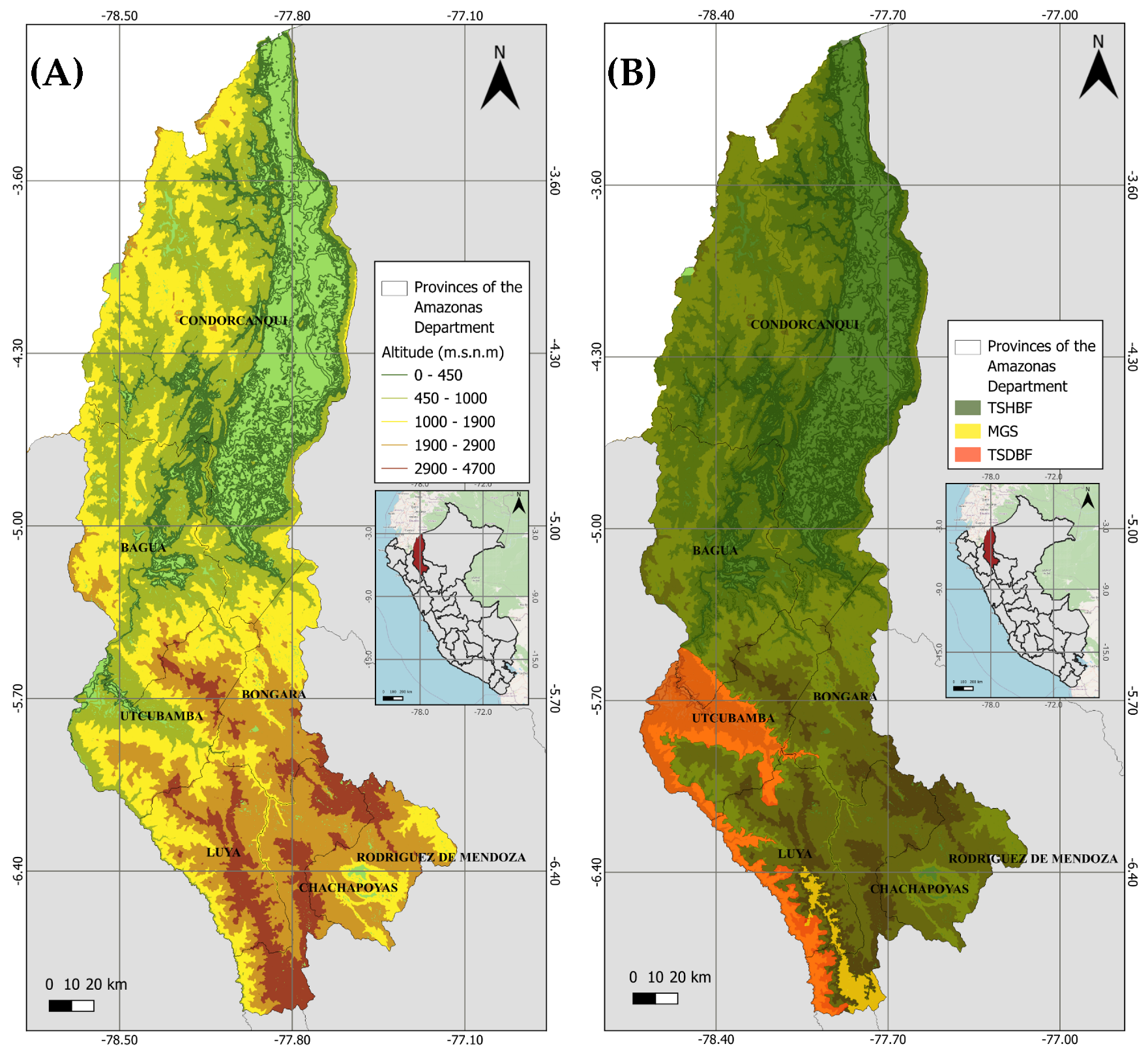
Figure 1. Study area in the Amazonas department, northern Peru. (A) Altitudinal distribution showing elevation ranges and provincial boundaries. (B) Distribution of the main ecoregions considered in this study: Tropical and Subtropical Humid Broadleaf Forests (TSHBF), Tropical and Subtropical Dry Broadleaf Forests (TSDBF), and Montane Grasslands and Shrublands (MGS).
Land 15 01745 g001
Figure 2. Workflow adopted for climate data processing and analysis.
Land 15 01745 g002
Figure 3. Temporal evolution of annual mean temperature (A), annual accumulated precipitation (B), and annual incoming shortwave solar radiation (C) during the historical period (1985–2014) and under the SSP2-4.5 and SSP5-8.5 scenarios (2015–2100). Thick solid lines represent the multi-model ensemble means, whereas coloured dashed lines represent the individual CMIP6 models. Shaded areas indicate the inter-model spread (±1 standard deviation). Vertical dashed lines delimit the historical, near-future, and far-future periods.
Land 15 01745 g003
Figure 4. Spatial distribution of annual mean air temperature (Tas) simulated by five CMIP6 Global Climate Models (CESM2, IPSL-CM6A-LR, MIROC6, MPI-ESM1-2-HR, and MRI-ESM2-0) and the multi-model ensemble for the historical period (1985–2014) and future climate projections (2031–2060 and 2071–2100) under the SSP2-4.5 and SSP5-8.5 scenarios.
Land 15 01745 g004
Figure 5. Spatial distribution of annual accumulated precipitation (Pr) simulated by five CMIP6 Global Climate Models (CESM2, IPSL-CM6A-LR, MIROC6, MPI-ESM1-2-HR, and MRI-ESM2-0) and the multi-model ensemble for the historical period (1985–2014) and future climate projections (2031–2060 and 2071–2100) under the SSP2-4.5 and SSP5-8.5 scenarios.
Land 15 01745 g005
Figure 6. Spatial distribution of annual incoming shortwave solar radiation (Rsds) simulated by five CMIP6 Global Climate Models (CESM2, IPSL-CM6A-LR, MIROC6, MPI-ESM1-2-HR, and MRI-ESM2-0) and the multi-model ensemble for the historical period (1985–2014) and future climate projections (2031–2060 and 2071–2100) under the SSP2-4.5 and SSP5-8.5 scenarios.
Land 15 01745 g006
Figure 7. Projected spatial anomalies of annual mean air temperature ( Δ Tas), annual accumulated precipitation ( Δ Pr), and annual incoming shortwave solar radiation ( Δ Rsds) relative to the historical period (1985–2014). (A) Δ Tas, SSP2-4.5, 2031–2060; (B) Δ Pr, SSP2-4.5, 2031–2060; (C) Δ Rsds, SSP2-4.5, 2031–2060; (D) Δ Tas, SSP5-8.5, 2031–2060; (E) Δ Pr, SSP5-8.5, 2031–2060; (F) Δ Rsds, SSP5-8.5, 2031–2060; (G) Δ Tas, SSP2-4.5, 2071–2100; (H) Δ Pr, SSP2-4.5, 2071–2100; (I) Δ Rsds, SSP2-4.5, 2071–2100; (J) Δ Tas, SSP5-8.5, 2071–2100; (K) Δ Pr, SSP5-8.5, 2071–2100; (L) Δ Rsds, SSP5-8.5, 2071–2100.
Land 15 01745 g007
Figure 8. Comparison of annual mean air temperature (A), annual accumulated precipitation (B), and annual incoming shortwave solar radiation (C) among the three ecoregions of the Amazonas department under the historical climate (1985–2014) and future climate projections (2031–2060 and 2071–2100) for the SSP2-4.5 and SSP5-8.5 scenarios. Bars represent the spatial mean for each ecoregion, and error bars indicate the spatial standard deviation within each ecoregion.
Land 15 01745 g008
Figure 9. Projected climate change, inter-model variability, and directional agreement under SSP5-8.5 for 2071–2100 relative to the historical baseline (1985–2014). Panels (AC) show the multi-model mean projected changes in annual mean air temperature, annual accumulated precipitation, and incoming shortwave solar radiation, respectively. Panels (DF) show the standard deviation across the five model-specific projected changes. Panels (GI) show directional agreement, expressed as the percentage of models whose sign of change agrees with the sign of the multi-model mean.
Land 15 01745 g009
Table 1. Global Climate Models (GCMs) used in this study.
ModelInstitutionCountryNative ResolutionReference
CESM2NCARUSA1.25° × 0.94°[21]
IPSL-CM6A-LRIPSLFrance2.5° × 1.27°[22]
MIROC6MIROC ConsortiumJapan1.4° × 1.4°[23]
MPI-ESM1-2-HRMPI-MGermany0.94° × 0.94°[24]
MRI-ESM2-0MRIJapan1.125° × 1.125°[25]
Table 2. Historical evaluation of the NEX-GDDP-CMIP6 multi-model ensemble against CHELSA v2.1 for 1985–2014.
VariableCHELSANEX-MMEBiasMAERMSEr
Temperature (°C)19.7121.752.042.132.570.943
Precipitation (mm yr−1)1903.11486.8 416.3 520.9639.30.660
Solar radiation (W m−2)197.7229.631.8631.8632.500.321
Note: CHELSA and NEX-MME columns represent area-weighted spatial means. NEX-MME denotes the arithmetic multi-model ensemble mean. Bias is NEX-MME minus CHELSA; therefore, positive values indicate overestimation and negative values indicate underestimation. MAE = mean absolute error; RMSE = root mean square error; r = area-weighted spatial Pearson correlation coefficient.
Table 3. Projected mean changes in annual mean temperature (Tas), annual accumulated precipitation (Pr), and incoming shortwave solar radiation (Rsds) relative to the historical period (1985–2014) in the Amazonas department.
VariableSSP2-4.5SSP5-8.5
2031–20602071–21002031–20602071–2100
Δ Tas (°C)1.202.121.533.96
Δ Pr (mm yr−1)56.86141.2784.06223.50
Δ Pr (%)3.9310.525.9716.59
Δ Rsds (W m−2)0.751.171.072.07
Notes: Tas = near-surface air temperature; Pr = annual accumulated precipitation; Rsds = incoming shortwave solar radiation. Δ Tas and Δ Rsds represent absolute changes relative to the historical period. For precipitation, both the absolute change (mm yr−1) and the mean cellwise relative change (%) are reported.
Table 4. Mean climatic conditions across the three ecoregions of the Amazonas department during the historical and future periods. Values are expressed as spatial mean ± standard deviation.
VariableEcoregionHistorical 1985–2014SSP2-4.5 2031–2060SSP2-4.5 2071–2100SSP5-8.5 2031–2060SSP5-8.5 2071–2100
Temperature (°C)
TSHBF21.98 ± 3.2323.18 ± 3.2324.10 ± 3.2423.51 ± 3.2425.95 ± 3.26
TSDBF20.23 ± 3.4121.41 ± 3.4122.28 ± 3.4121.72 ± 3.4024.07 ± 3.40
MGS14.14 ± 1.1415.36 ± 1.1316.24 ± 1.1315.67 ± 1.1318.05 ± 1.13
Precipitation (mm yr−1)
TSHBF1553.98 ± 596.841613.39 ± 615.051697.92 ± 622.261640.91 ± 621.101781.98 ± 640.63
TSDBF786.46 ± 72.53815.06 ± 73.82895.31 ± 75.11837.04 ± 73.73953.23 ± 82.15
MGS787.77 ± 17.04830.88 ± 20.44934.39 ± 29.80868.01 ± 25.121034.68 ± 46.87
Solar radiation (W m−2)
TSHBF229.11 ± 3.02229.88 ± 2.87230.37 ± 2.61230.22 ± 2.81231.35 ± 2.27
TSDBF234.26 ± 0.96234.72 ± 0.87234.55 ± 0.75234.86 ± 0.81234.59 ± 0.56
MGS233.81 ± 0.71234.45 ± 0.68234.32 ± 0.65234.62 ± 0.66234.25 ± 0.50
Notes: TSHBF = Tropical and Subtropical Humid Broadleaf Forests; TSDBF = Tropical and Subtropical Dry Broadleaf Forests; MGS = Montane Grasslands and Shrublands. Values represent spatial summaries within each ecoregion. Standard deviations describe spatial variability within each ecoregion and do not represent inter-model variability.
Table 5. Climate hotspot thresholds and hotspot extent within the three ecoregions under SSP5-8.5 for 2071–2100 relative to the historical baseline (1985–2014).
Variable P 75 ThresholdTSHBF (%)TSDBF (%)MGS (%)
Temperature4.04 °C27.380.000.00
Precipitation18.59%21.5653.77100.00
Solar radiation2.69 W m−227.420.000.00
Notes: P 75 = 75th-percentile threshold calculated across the Amazonas department. Percentages represent the proportion of the represented area of each ecoregion classified as hotspot. TSHBF = Tropical and Subtropical Humid Broadleaf Forests; TSDBF = Tropical and Subtropical Dry Broadleaf Forests; MGS = Montane Grasslands and Shrublands.
Disclaimer/Publisher’s Note: The statements, opinions and data contained in all publications are solely those of the individual author(s) and contributor(s) and not of MDPI and/or the editor(s). MDPI and/or the editor(s) disclaim responsibility for any injury to people or property resulting from any ideas, methods, instructions or products referred to in the content.